Resonances from Quiver Theories at the LHC

Abstract

We consider the collider signals of spin-one resonances present in full-hierarchy quiver theories of electroweak symmetry breaking. These four-dimensional theories result from the deconstruction of warped extra dimensional models and have very distinct phenomenological features when the number of sites is small. We study a class of generic scenarios in these theories where the color gauge group as well as the electroweak sector, propagate in the quiver diagram. These scenarios correspond to various specific models of electroweak symmetry breaking and fermion masses. We focus on the minimum resonant content and its main features: the presence of heavy and narrow spin one resonances. We derive bounds from the LHC data on the color-octet and color-singlet excited gauge bosons from their decays to jets and top pairs, and show their dependence on the number of sites in the quiver. We also compare them with the bounds derived from flavor violation.

I Introduction

The electroweak standard model (SM) describes satisfactorily all available data to date pdg . Since it is a renormalizable theory, this implies that its cutoff $\Lambda$ –the scale of new physics– is far above the weak scale $v\simeq 246~{}$GeV. This has been most recently confirmed by the apparent discovery of a light Higgs boson with $m_{h}\simeq 126~{}$GeV higgsdicovery , which is compatible with the renormalizable SM Higgs sector. On the other hand, the resolution of the hierarchy problem requires that new physics beyond the SM appear at scales not too far above the TeV. This little hierarchy problem points to the need to have a parametric separation of the weak scale and the new physics scale. In non-supersymmetric theories the Higgs must be a remnant pseudo-Nambu Goldstone boson (pNGB) from the spontaneous breaking of a global symmetry chm . The resonances will then have higher masses as dictated by the gap between the pNGBs and the resonant sector in analogy with the $m_{\pi}-m_{\rho}$ mass gap. There are several scenarios beyond the SM with a pNGB Higgs. These include the Little Higgs littlehiggs , Twin Higgs twinhiggs , as well as extra-dimensional models where the Higgs is obtained from a bulk gauge field in what is sometimes called Gauge-Higgs Unification, particularly in AdS₅ backgrounds ghunification . In all cases, there will be a large global symmetry spontaneously broken giving rise to NGBs. Part of this global symmetry is gauged and therefore explicitly broken. This allows for a partial Higgs mechanism eliminating some of the NGBs to give masses to the gauge bosons associated with broken generators, and at the same time leads to a potential for the Higgs and its small mass. For the model to be successful, there must be a set of NGBs left out in the spectrum forming a doublet of $SU(2)_{L}$ that can be identified with the Higgs field responsible for EWSB.

The gap between $m_{h}$ and the resonant masses is a generic feature of all these scenarios. The tell-tale of the details of the underlying dynamics is in the resonant spectrum and couplings. It is possible to parametrize these dynamics in an effective field theory framework of the low energy symmetries of the SM. This has been done in several papers silh .

In this paper we will commit to a more specific set of models including a pNGB Higgs. These theories can be represented by quiver (or moose) diagrams quiver1 ; quiver2 (see next section), and are cousins of AdS₅ models since there is a limit in which the two are essentially identical. In these limit, the quiver theories are obtained from the deconstruction decon ; bbh of AdS₅ theories. However, far form this continuum limit, in what we can call the coarse limit, quiver theories are four-dimensional and quantitatively very different from the AdS₅ ones. In particular, the spectrum and couplings of the resonant states –both bosonic and fermionic– will be significantly different than for the continuum case, and in general dependent upon the number of gauge groups (or “sites” in the quiver diagram), as well as the group structure and matter representation chosen. Then, in the coarse deconstruction limit, quiver theories will have a very distinctive phenomenology at the LHC. We will begin exploring this phenomenology in vanilla quiver models as the ones presented in Refs. quiver1 and quiver2 . We will concentrate on the production of vector resonances decaying into quarks giving jets and $t\bar{t}$ pairs, as this should be the first signal for these models at the LHC (as we show below).

The phenomenology of quiver or moose theories has been studied in many other papers, but in different setups. For instance, in Ref.  higgsless3site a three-site electroweak model without a Higgs is built, and its phenomenology is studied in  higgslesspheno . Its generalization to allow for a light Higgs is presented in Ref. hthreesite . This “221” model is a very specific quiver theory, and although there are quite a few common points with our work, we will always consider larger gauge groups a a set of ordered vacua. In Ref. fdcompositeh a two-site quiver is proposed, its phenomenology of the extended gauge sector studied in Ref. fdcpheno . A three-site construction more similar to ours is that of Ref. dischm . Our approach differs from all these previous contributions in one way or the other already at the model building stage. We are considering generic coarse deconstruction models with a very high ultra-violet cutoff. Our studies allow to consider the number os sites as a variable. Our aim is to start a systematic study of the phenomenology of quiver theories by pointing out their main common features: narrow resonances as a result of weak coupling, compatibility with flavor physics resulting in specific decay channels, and a Higgs sector compatible with a pNGB light Higgs. It is possible that some of our results can be partially applied to the models mentioned above.

In the next section, we present the general framework for quiver theories, and we specify one model to study its phenomenology. In Section III, we obtain the couplings of vector resonances to SM fields, and in particular to SM quarks. We also obtain the resonance widths. These results are used in Section IV to extract the current bounds on the model spectrum from di-jet and $t\bar{t}$ resonance searches at ATLAS and CMS. We give our conclusions and outlook in Section V.

II The Model Framework

We begin this section by reviewing the basics of quiver theories (QT). Let us consider the product gauge group $G_{0}\times G_{1}\times\cdots G_{j}\times G_{j+1}\cdots G_{N}$. In addition, we have a set of scalar link fields $\Phi_{j}$, with $j=1~{}{\rm to~{}}N$, transforming as bi-fundamentals under $G_{j-1}\times G_{j}$. The action for the theory is

$$S = \int d^{4}x\left\{-\,\sum_{j=0}^{N}\,\frac{1}{2g_{j}^{2}}\,Tr\left[F_{\mu\nu}^{(j)}F^{\mu\nu(j)}\right]\right.$$ (1)

$$\left.+\sum_{j=1}^{N}\,Tr\left[(D_{\mu}\Phi_{j})^{\dagger}D^{\mu}\Phi_{j}\right]-V(\Phi_{j})+\dots\right\}$$

where the traces are over the groups’ generators, and the dots at the end correspond to terms involving fermions and will be discussed in the next section. We assume that the potentials for the link fields give each of them a vacuum expectation value (VEV) which breaks $G_{j-1}\times G_{j}$ down to the diagonal group, and result in non-linear sigma models for the $\Phi$’s

$$\Phi_{j}=\frac{v_{j}}{\sqrt{2}}\,e^{i\sqrt{2}\pi_{j}^{a}\hat{t}^{a}/v_{j}}~{},$$ (2)

where the $\hat{t}^{a}$’s are the broken generators, the $\pi_{j}^{a}$ the Nambu-Goldstone Bosons (NGB); and $v_{j}$ are the VEVs of the link fields. We will consider here the situation where the VEVs are ordered in such a way that $v_{1}>v_{2}\dots>v_{j}\dots>v_{N}$. We parametrize the ordering by defining the VEVs as

$$v_{j}\equiv vq^{j}~{},$$ (3)

where $0<q<1$ is a dimensionless constant, and $v$ is a UV mass scale that can be regarded as the UV cutoff. We will also assume for the moment that all the gauge groups are identical and that their gauge couplings satisfy

$$g_{0}(v)=g_{1}(v_{1})=\dots=g_{j}(v_{j})=g_{j+1}(v_{j+1})=\dots\equiv g~{}.$$ (4)

The model can be illustrated by the quiver diagram of Figure 1.

Figure 1: Quiver diagram for the theory described by Eq. (1).

The gauge boson mass matrix squared is given by

$$M^{2}_{g}\,=\,g^{2}\,v^{2}\,\left(\begin{array}[]{ccccccc}q^{2}&-q^{2}&0&0&\cdots&0&0\\ -q^{2}&q^{2}+q^{4}&-q^{4}&0&\cdots&0&0\\ 0&-q^{4}&q^{4}+q^{6}&-q^{6}&\cdots&0&0\\ \vdots&\vdots&\vdots&\vdots&\cdots&\vdots&\vdots\\ 0&0&0&0&\cdots&q^{2(N-1)}+q^{2N}&-q^{2N}\\ 0&0&0&0&\cdots&-q^{2N}&q^{2N}\end{array}\right)\,.$$ (11)

in the basis $(A_{0},A_{1},\cdots,A_{N})$, and in the unitary gauge. We diagonalize $M_{g}$ by the orthonormal rotation

$$A^{j}_{\mu}=\sum_{n=0}^{N}f_{j,n}A^{(n)}_{\mu}~{},$$ (12)

where the $\{A_{\mu}^{(n)}\}$ are the mass eigenstates. The zero-mode gauge boson, $A_{\mu}^{(0)}$, has a “flat profile” in the quiver diagram, meaning that for all $j$ $f_{j,0}=1/\sqrt{N+1}$. This is not the case for the massive modes, for which $f_{j,n}$ can be obtained from the diagonalization procedure. In order to address the hierarchy problem, we will need that the first gauge excitation is $v_{N}\simeq O(1)~{}$TeV. Furthermore, if we impose that these models are to address the full hierarchy between the Planck and the electroweak scales, then $v\begin{array}[]{c}\,\sim\vspace{-1.7em}\\ <\end{array}M_{P}$. Thus, the values of the model parameter $q$ and the number of gauge groups $N$ would be related by

$$q=10^{-16/N}~{}.$$ (13)

The Higgs field will have to have a profile highly localized towards the site $N$, in order for the corrections to its mass to be no larger than of order of the electroweak scale. In a full model this can be done dynamically by extracting the Higgs doublet from a NGB that stays in the spectrum quiver2 . Here, we will make the simplification of assuming that the Higgs doublet only transforms under the weak gauge group of site $N$, i.e. is completely “localized” on the site $N$. This simplifying assumption will be of little impact on the rest of the paper.

In the limit of large $N$, and $q\rightarrow 1_{-}$, these models can be described by the deconstruction decon1 of theories with one compact extra dimension in an AdS background, AdS₅ rs . The deconstruction of AdS₅ was studied in Refs. decon1 ; bbh ; tools . This continuum limit, in which the four-dimensional theory described above and the AdS₅ theories are equivalent, is obtained when the ultra-violet (UV) scale of the 4D theory, which is approximately $v$, is larger than the curvature $k$ of the 5D AdS space: $k<v$. In fact, in the language of the deconstructed theory obtained by discretizing AdS₅, $v$ corresponds to the inverse of the discretization interval $a$. Using Eq. (13) and the identification $q\leftrightarrow e^{-k/gv}$ decon ; bbh ; quiver1 necessary for matching both theories, we see that for $N\begin{array}[]{c}\,\sim\vspace{-1.7em}\\ >\end{array}36$ the quiver theories would be essentially identical to the extra-dimensional theory in AdS₅. On the other hand, for smaller values of $N$ the 4D theories cannot be interpreted as AdS₅ ones and should be studied separately.

The introduction of fermions in these models was extensively studied in Refs. bbh ; quiver1 . The fermion action is given by

$$S_{f} = \int d^{4}x\sum_{j=0}^{N}\left\{\bar{\psi}_{L}^{j}i\not D_{j}\psi_{L}^{j}+\bar{\psi}_{R}^{j}i\not D_{j}\psi_{R}^{j}\right.$$ (15)

$$\left.-(\mu_{j}\bar{\psi}_{L}^{j}\psi_{R}^{j}+\lambda_{j}\bar{\psi}_{R}^{j-1}\Phi_{j}\psi_{L}^{j}+{\rm h.c.})\right\}~{},$$

where the $\mu_{j}$ are vector-like masses and the Yukawa couplings are chosen in such a way so as to only result in one zero mode fermion bbh . For a left-handed zero-mode, the “boundary condition” must be chosen such that $\psi_{R}^{N}=0$. Conversely, to obtain a right-handed zero mode fermion, the condition is $\psi_{L}^{0}=0$. A schematic diagram of the fermionic action is shown in Figure 2 for a left-handed zero mode.

Figure 2: Quiver diagram for the theory described by Eq. (15), with a left-handed zero mode fermion.

By using Eq. (2), we can obtain the fermion mass matrix, which just as for the case of gauge bosons is not diagonal due to the mixing induced by the VEVs of the link fields $\Phi_{j}$. The rotation to a mass-eigenstate basis is defined as

$$\psi_{L,R}^{j}=\sum_{n=0}^{N}h_{L,R}^{j,n}\,\chi_{L,R}^{(n)}~{},$$ (16)

where the $\chi_{L,R}^{(n)}$ are the mass eigenstates. We are interested in the coefficients $h_{L,R}^{j,0}$ corresponding to the zero-mode localization in the quiver diagram. They can be chosen so as to obtain the correct fermion masses and mixings considering that the Higgs is highly localized close to the site $N$. For instance, the situation with the Higgs localized at site $N$ was studied in Ref. quiver1 for the quark sector. From the equations of motion it is possible to obtain relations among the zero-mode coefficients. In general, the zero-mode coefficients for the left and right handed cases satisfy:

$$\sqrt{2}\frac{\mu_{j}}{v\lambda_{j+1}} = -q^{j+1}\,\frac{h_{L}^{j+1,0}}{h_{L}^{j,0}}$$ (17)

$$\sqrt{2}\frac{\mu_{j}}{v\lambda_{j}} = -q^{j}\,\frac{h_{R}^{j-1,0}}{h_{R}^{j,0}}~{}.$$ (18)

The choice of fermion localization can then be parametrized in order to get the desired ratios in Eqns. (17) and (18). For instance, we choose the parametrizations

$$\frac{h_{L}^{j+1,0}}{h_{L}^{j,0}}=q^{c_{L}-1/2}~{},\qquad\frac{h_{R}^{j,0}}{h_{R}^{j-1,0}}=q^{-(c_{R}+1/2)}~{},$$ (19)

which in the continuum limit would result in fermion zero-mode wave functions parametrized by $c_{L}$ and $c_{R}$ defined in rs . As mentioned above, the localization parameters $c_{L}$ and $c_{R}$ are chosen so as to obtain the observed pattern of fermion masses and mixings for a given Higgs localization model. This can be a simple N-localized Higgs as in Ref. quiver1 , or the dynamically localized pNGB as in Ref. quiver2 .

In the next section we will obtain the couplings of zero-mode fermions (the SM fermions) to the first excitation of gauge bosons so we can study their phenomenology at the LHC.

III Resonances in Quiver Theories

We are interested in obtaining the couplings of the massive gauge boson resonances to the SM fermions. We follow closely Ref. quiver1 . The couplings are defined by

$$g^{01}_{L,R}\,\bar{\chi}_{L,R}^{(0)}\gamma^{\mu}A_{\mu}^{(1)}\chi_{L,R}^{(0)}~{},$$ (20)

where we assumed that the group generators are absorbed in the definition of the gauge fields. The wave-function of a zero-mode fermion can be written in terms of the quiver fermions as

$$\chi^{(0)}_{L,R}=\sum_{j=0}^{N}\,h_{L,R}^{*j,0}\,\psi_{L,R}^{j}~{}.$$ (21)

In the same way, and assuming a generic gauge group in the sites of the quiver diagram, the mass-eigenstates of the gauge bosons can be written in terms of the quiver gauge bosons as

$$A_{\mu}^{(n)}=\sum_{j=0}^{N}\,f^{*}_{j,n}\,A^{j}_{\mu}~{},$$ (22)

with $f_{j,n}$ the coefficient linking the gauge boson in site $j$ with the mass-eigenstate $n$ in the rotation to mass eigenstates. Therefore, the coupling of the $n=1$ massive gauge boson to the zero-mode fermions is

$$g^{01}_{L,R}=\sum_{j=0}^{N}\,g_{j}\,\left|h_{L,R}^{j,0}\right|^{2}\,f_{j,1}~{},$$ (23)

where $g_{j}$ are the gauge couplings associated to the group $G_{j}$ in the quiver and as mentioned before, we assume $g_{j}=g$ for all $j$ in the manner defined by Eq. (4). The coefficients $f_{j,1}$ can be obtained by diagonalizing the gauge boson mass matrix tools ; bbh for a given $N$. Then, we can obtain the couplings of zero-mode fermions to the first excited state of the gauge bosons, normalized by the gauge coupling $g$.

In Figure 3 we show the couplings of the left-handed zero-mode fermions to the first excited gauge boson state, $g^{L}_{01}$, normalized to the zero-mode gauge coupling and for $N=4$, $9$ and $15$, as a function of the fermion localization parameter $c_{L}$ defined by Eqs. (19).

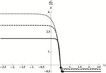
Figure 3: The couplings of left-handed zero-mode fermions to the first excited gauge bosons as a function of the fermion localization parameter $c_{L}$, for $N=4~{}\mathrm{(solid)},$ $N=9~{}\mathrm{(dashed)},$ and $N=15~{}\mathrm{(dotted)}$. The dots correspond to the localizations for a solution for the $N=4$ case and are shown as an illustration.

The values of the localization parameter above $c_{L}=0.5$ correspond to “UV” zero-mode localization: most of the zero-mode wave function comes from fermions transforming under gauge groups that are associated with larger VEVs. Conversely, for $c_{L}<0.5$ the zero-mode fermion wave-function is mostly coming from fermions transforming under gauge groups associated with smaller VEVs. We refer to the latter as “IR” localization.

Similarly, in Figures 4 and  5 we show the couplings of up and down right-handed zero-mode fermions to the first gauge boson excitation, as a function of the respective $c_{R}$ localization parameters.

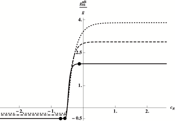
Figure 4: The couplings of up-type right-handed zero-mode fermions to the first excited gauge bosons as a function of the fermion localization parameter $c_{R}$, for $N=4~{}\mathrm{(solid)},$ $N=9~{}\mathrm{(dashed)},$ and $N=15~{}\mathrm{(dotted)}$.

In these cases, localization parameters with values $c_{R}<-0.5$, correspond to “UV” localization in the quiver, whereas for $c_{R}>-0.5$, most of the zero-mode wave function comes from fermions transforming under “IR” gauge groups.

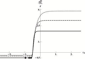
Figure 5: The couplings of down-type right-handed zero-mode fermions to the first excited gauge bosons as a function of the fermion localization parameter $c_{R}$, for $N=4~{}\mathrm{(solid)},$ $N=9~{}\mathrm{(dashed)},$ and $N=15~{}\mathrm{(dotted)}$.

The localizations illustrated by three points in Figures 3,  4 and  5 correspond to a given solution for the localizations of the zero-mode quarks for $N=4$. This solution is consistent with the quark mass spectrum, the CKM matrix elements and has minimal flavor-changing neutral current effects quiver1 . Similar solutions can be found for the other values of $N$.

As it can be seen in the Figures above, the couplings of IR-localized zero-mode fermions increase with $N$, whereas the ones corresponding to UV-localized, decrease. In the continuum limit, which as we noted in the previous section is reached for $N\begin{array}[]{c}\,\sim\vspace{-1.7em}\\ >\end{array}36$, the couplings will behave exactly as those in AdS₅ bulk models rs . However, and as it was shown in Ref. quiver1 , for coarse deconstruction ($N<36$), the resulting models have a different quantitative behavior. For instance, flavor violation can be easily accommodated with mass scales above just a few TeV (specifically, $M_{G}>3~{}$TeV for $N=4$ with $M_{G}$ the mass of the first excitation of the gluon), whereas the continuum requires typically higher mass scales for the Kaluza-Klein states.

We can also see that the widths of the first excitations of gauge bosons will not be as dominated by third generation channels as in the continuum case. On one hand, the light UV-localized quarks leading to jets have couplings to the excitation that are not as suppressed as in the continuum case. Furthermore, the third generation couplings are not as large. In addition, the overall values of the couplings are smaller, leading to significantly smaller total widths. Typical widths for the first gauge excitations are $\Gamma/M\simeq 0.05$. These facts result in a distinct phenomenology for resonance production and decay when compared with the AdS₅ case. For quiver theories, resonances will be narrow and with significant di-jet signals. There will be still important contributions to the $b\bar{b}$ and $t\bar{t}$ channels. The latter might even dominate the bounds in some cases, as we will see below.

In the next section, we use the couplings computed here to obtain the s-channel production of the first-excited states of the gauge bosons at the LHC into jets and $t\bar{t}$ final states.

IV Resonances from Quiver Theories at the LHC

In this section we study the production of the first excited state of the gauge bosons from full-hierarchy quiver theories at the LHC. We will consider two cases of particular interest.

The first case, corresponds to the quiver gauge group with ${\cal G}=SU(3)^{N+1}$, broken down to the QCD gauge group, ${\cal G}\rightarrow SU(3)_{c}$. The zero-mode gauge boson is the SM gluon, and the tower of excited states are massive color-octet spin-1 resonances. This can be seen as the coarse deconstruction of bulk QCD in AdS₅. The reason to study this case is partly phenomenological: since they are color-octet states they will have larger production cross sections. It also serves as comparison with the extra-dimensional case in AdS₅ models with bulk $SU(3)_{c}$ gauge fields. However, unlike in the AdS₅ case, it is not necessary for $SU(3)_{c}$ to “propagate” in the quiver. It is entirely possible to obtain a quiver model of EWSB and fermion masses with a pNGB Higgs boson without a color-octet tower.

The second case corresponds to having the quiver gauge group ${\cal G}=(SU(2)_{L}\times U(1)_{Y})^{N+1}$, broken to the electroweak SM gauge group: ${\cal G}\rightarrow SU(2)_{L}\times U(1)_{Y}$. The zero-mode gauge bosons in this case are the electroweak gauge bosons before EWSB, with them replicated in the tower of excited states. The interest in this second case resides on the fact that, although in quiver models where the Higgs is a pNGB quiver2 the quiver gauge groups must be larger than the SM gauge group in order to extract the Higgs from un-eaten NGBs, the massive states will contain these ones as a subset. Thus, studying the phenomenology of these massive states is independent of the particular model chosen for the electroweak quiver.

We will compute the cross section for production and decay to a given channel for the color-octet and electroweak first vector resonances at the LHC with $\sqrt{s}=8~{}$TeV, for various values of the number of sites $N$. We concentrate on channels with quarks in the final state, leading to light jets and $t\bar{t}$ final states. We leave out for now $b\bar{b}$ final states since there will be less constraining. In each case the couplings to the SM quarks, the zero-mode quarks in the model as presented above, is computed assuming a quark localization in the quiver consistent with the correct mass matrix and CKM mixing. These solutions for each value of $N$ are then consistent with all flavor phenomenology.

The resonance widths are quite small in all cases. This is to be compared to the AdS₅ situation where typical widths for the Kaluza-Klein gluon are well above the typical resolution kkgwidth . We start with the color-octet excited states.The production cross section times the branching ratio into jets is shown in Figure 6, for three choices of the number of gauge groups in the quiver: $N=4$ (5 gauge groups), $N=9$ and $N=15$.

Figure 6: The dijet production cross section times branching ratio for $\sqrt{s}=8~{}$TeV, as a function of the color-octet mass for $N=4~{}\mathrm{(solid)},$ $N=9~{}\mathrm{(dashed)},$ and $N=15~{}\mathrm{(dotted)}$.

The corresponding plots for the color-octet production decaying into a $t\bar{t}$ pairs is shown in Figure 7.

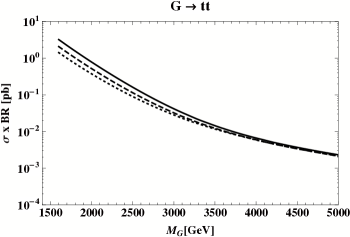
Figure 7: The $t\bar{t}$ production cross section times branching ratio for $\sqrt{s}=8~{}$TeV, as a function of the color-octet mass for $N=4~{}\mathrm{(solid)},$ $N=9~{}\mathrm{(dashed)},$ and $N=15~{}\mathrm{(dotted)}$.

We also consider color-singlet states, as mentioned earlier, as a combination of the first excitation of the photon and the $Z$, $(Z^{\prime}+\gamma^{\prime})$, since these are likely to be close in mass. In Figure 8, we show the production times branching ratios for $(Z^{\prime}+\gamma^{\prime})$ decaying to di-jets for several choices of $N$.

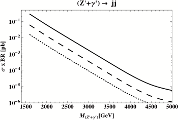
Figure 8: The di-jet production cross section times branching ratio for $\sqrt{s}=8~{}$TeV, as a function of the $(Z^{\prime}+\gamma^{\prime})$ mass for $N=4~{}\mathrm{(solid)},$ $N=9~{}\mathrm{(dashed)},$ and $N=15~{}\mathrm{(dotted)}$.

A similar plot for the decays of the color-singlet into top pairs is shown in Figure 9.

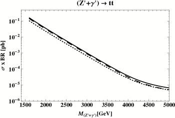
Figure 9: The $t\overline{t}$ production cross section times branching ratio $\sqrt{s}=8~{}$TeV, as a function of the $(Z^{\prime}+\gamma^{\prime})$ mass for $N=4~{}\mathrm{(solid)},$ $N=9~{}\mathrm{(dashed)},$ and $N=15~{}\mathrm{(dotted)}$.

In the case of the di-jet decay channels, both for the color-octet as well as for the color-singlet, we can see that as the number of sites in the quiver diagram ($N$) grows, the $\sigma\times\rm{BR}$ falls (Figures 6 and 8). This is to be expected, since as $N$ grows and we approach the continuum AdS₅ limit the size of the light quark couplings to the first gauge excitation diminishes. On the other hand, the corresponding $t\bar{t}$ decay channels are much more degenerate, as it can be seen in Figures 7 and 9. This is due to the fact that the top couplings to the first gauge excitation grow with $N$, which almost exactly compensates the reduction in production cross section coming from smaller light-quark couplings.

We derive bounds from the LHC data accumulated with $\sqrt{s}=8~{}\mathrm{TeV}$. In particular, we use the CMS bounds on di-jets resonances of Ref. CMSjj , which uses $19.6~{}\mathrm{fb}^{-1}$ of integrated luminosity, whereas we use the bounds obtained by ATLAS on $t\bar{t}$ resonances Atlastt with an integrated luminosity of $14.5~{}\mathrm{fb}^{-1}$. Since the quiver resonances are narrow interference effects can be neglected. Moreover, in order to compare with the experimental limits we must only consider the resonance region since the bounds are obtained by “bump searches”. Table 1 shows the direct bounds from LHC on the color-octet mass. These are obtained from the CMS constraints on di-jet resonances in Ref. CMSjj , and from the ATLAS bounds on $t\bar{t}$ resonances of Ref. Atlastt .

Table 1: Bounds on the color-octet mass [TeV].

$N$	Dijet CMSjj	$t\overline{t}$ Atlastt
4	3.0	2.7
9	1.6	2.6
15	–	2.5

We see that, unlike for the KK gluon in AdS₅ models, the di-jet bounds are competitive, being the best limit in the $N=4$ case. As mentioned above, the bounds coming from $t\bar{t}$ are not really sensitive to $N$. All of the bounds on quiver resonances from Table 1 are similar to the flavor and electroweak precision bounds obtained in Ref. quiver1 , which were typically $\sim 3$ TeV.

We also consider the bounds on first electroweak gauge boson excitations. As mentioned above, this sector typically contains at least an excitation of the $Z$ ($Z^{\prime}$) and one of the photon ($\gamma^{\prime}$), in addition to other weakly coupled first excitations not corresponding to any SM zero mode. Here we study the bounds on this minimum electroweak set of excitations, $Z^{\prime}$ and $\gamma^{\prime}$. Furthermore, we will assume that their masses are close enough to appear degenerate at the LHC, at least in the search stages. As a consequence, we will obtain bounds on the $Z^{\prime}+\gamma^{\prime}$ combination.

Table 2: Bounds on the ($Z^{\prime}$+$\gamma^{\prime}$) mass [TeV]

$N$	Dijet CMSjj	$t\overline{t}$ Atlastt
4	1.7	2.1
9	–	2.0
15	–	1.8

In Table 2 we show the bounds on the $(Z^{\prime}+\gamma^{\prime})$ combination from di-jets from CMS CMSjj , and from top pairs from ATLAS Atlastt . Once again, the di-jet channel is competitive for low values of the number of sites, but $t\bar{t}$ is most constraining in general. The entries without a bound, both in Table 2 as well as in Table 1, correspond to bounds that are too low for them to be consistent with flavor and electroweak limits, as well as other direct bounds.

We observe that the bounds obtained in Tables 1 and 2 are still below what is needed to pass flavor-violation bounds in most of these models ($\simeq 3$ TeV). This mass range will be probed by the next stage of the LHC, with higher energy and luminosity.

V Outlook and Conclusions

We have considered the phenomenology of a class of four-dimensional quiver theories quiver1 , related to AdS₅ bulk models rs by coarse deconstruction. In particular, we have studied the current bounds on gauge excitations in these theories imposed by using the current LHC data. To be as general as possible we considered two kinds of resonances. First, we studied a color-octet excitation which corresponds to the propagation of color $SU(3)$ in the quiver. Unlike in the extra-dimensional formulation, this propagation is not necessary. However, we consider this case for completeness and comparison to the AdS₅ case. Secondly, we studied the bounds on the minimal electroweak excitations of these models, namely a $Z$ and photon excitations. For simplicity, we assumed that these two are nearly degenerate, whereas their common mass need not be the same as that of the color-octet state. The rationale for this split in the spectrum is that corrections to the color-octet mass should in general be different and probably larger than the ones affecting the colorless states. This allows for the possibility that the color-octet state, which drives the flavor bounds quiver1 , is heavier than the electroweak excitations.

We treated the number of sites $N$ as a free parameter, as long as it satisfies coarseness, i.e. $N\leq 36$. In this way, the phenomenology of these spin-1 resonances is guaranteed to be qualitatively different from that of AdS₅ Kaluza-Klein states. The bounds obtained for the color-octet state and the weakly coupled combination $(Z^{\prime}+\gamma^{\prime})$ depend on the parameter $N$, and they appear in Tables 1 and 2. We see that in both cases the $t\bar{t}$ constraints are still consistently dominant. However, the di-jet bounds can be competitive for lower number of sites, for which the light quark couplings are not as suppressed. For instance, for $N=4$ ($5$ sites), the most stringent bound comes from the di-jet channel of the color-octet. Still in this case, we see that the bounds are not yet above the mass scale needed to suppressed flavor changing neutral current, typically $\begin{array}[]{c}\,\sim\vspace{-1.7em}\\ >\end{array}3$ TeV quiver1 .

For the colorless states the bounds obtained are somewhat smaller, as shown in Table 2. Although in principle these bounds are consistent with flavor violation in the quark sector, the most important constraints on these states will probably come from flavor violation in the lepton sector. However, these are not yet available for quiver theories, as their lepton sector is only now beginning to be considered in the literature leptons .

In order for direct searches to compete with the flavor bounds of Ref. quiver1 , it would be necessary to probe above the mass scale of about $3~{}$TeV. We conclude that to do this decisively, the higher energy run at the LHC will be necessary. To illustrate this point we show the cross sections for the production of the color-octet and color-singlet states studied in this paper, at $\sqrt{s}=14~{}$TeV, for the di-jet and $t\bar{t}$ channels.

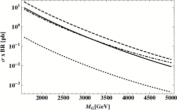
Figure 10: The color-octet production cross section times branching ratio as a function of the color-octet mass into di-jets for $N=4~{}\mathrm{(solid)},$ and $N=15~{}\mathrm{(dotted)}$; and into top pairs for $N=4~{}\mathrm{(dashed)}$ and $N=15~{}$(dot-dashed). All for $\sqrt{s}=14~{}$TeV.

In Figure 10 we show the color-octet production cross sections times branching fractions into di-jets for $N=4$ (solid) and $N=15$ (dotted), as well as the ones into $t\bar{t}$ for $N=4$ (dashed) and $N=15$ (dot-dashed). Although a careful study is necessary to know the reach of the LHC at $\sqrt{s}=14~{}$TeV for a given luminosity, we can see that the reach in the color-octet mass will be much above 3 TeV, perhaps as much as 5 TeV with a few hundred $\rm{fb}^{-1}$ of accumulated luminosity. Similarly, cross sections times branching fractions for the electroweak states $(Z^{\prime}+\gamma^{\prime})$, for $\sqrt{s}=14~{}$TeV are shown in Figure 11.

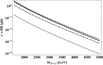
Figure 11: The color-singlet production cross section times branching ratio as a function of the color-singlet mass into di-jets for $N=4~{}\mathrm{(solid)},$ and $N=15~{}\mathrm{(dotted)}$; and into top pairs for $N=4~{}\mathrm{(dashed)}$ and $N=15~{}$(dot-dashed). All for $\sqrt{s}=14~{}$TeV.

We have seen that the quiver theories studied here are phenomenologically distinct from AdS₅ models. In particular, the existence of rather narrow resonances even in the color-octet case would point to states very different from a Kaluza-Klein gluon. Quiver theories generalize the model building philosophy of AdS₅ models of electroweak symmetry breaking and fermions masses. The spin-1 resonances studied here should be among the first signals for these kind of physics. Other signals, parametrized by the number of sites $N$, would follow. Their study would depend on details of the models, such as fermion representations chosen, the model building of the lepton sector leptons and the Higgs sector quiver2 , just to mention a few. Ultimately, quiver theories form a class of theories beyond the SM which includes AdS₅ as the continuum limit. Thus, their phenomenology at the LHC should be treated together. For instance, the presence of a set of signals for new physics could determine the value of $N$ (if any) consistent with all of them. The theoretical interpretation of this value, whether indicating a continuum theory or a coarse quiver one, would be an important step in determining the road to build the right theory of the TeV scale.

Acknowledgments The authors acknowledge the support of the State of São Paulo Research Foundation (FAPESP), the Brazilian National Council for Technological and Scientific Development (CNPq), and the Brazilian Agency for Postgraduate Development (CAPES).

References

- (1) J. Beringer et al. [Particle Data Group Collaboration], Phys. Rev. D 86, 010001 (2012).
-
(2)
G. Aad et al. ATLAS Collaboration,
Phys. Lett. B 716, 1 (2012)
[arXiv:1207.7214 [hep-ex]];
ATLAS Collaboration, Science 338, 1576 (2012);
S. Chatrchyan et al. CMS Collaboration, arXiv:1303.4571 [hep-ex];
S. Chatrchyan et al. CMS Collaboration, Science 338, 1569 (2012). - (3) D. B. Kaplan and H. Georgi , Phys. Lett. B 136, 183 (1984).
-
(4)
N. Arkani-Hamed, A. G. Cohen, E. Katz,
A. E. Nelson, T. Gregoire and J. G. Wacker ,
JHEP 0208, 021 (2002)
[hep-ph/0206020];
D. E. Kaplan, M. Schmaltz and , JHEP 0310, 039 (2003) [hep-ph/0302049];
For a review see M. Schmaltz and D. Tucker-Smith, Ann. Rev. Nucl. Part. Sci. 55, 229 (2005) [hep-ph/0502182]. -
(5)
Z. Chacko, H. -S. Goh and R. Harnik,
Phys. Rev. Lett. 96, 231802 (2006)
[hep-ph/0506256];
Z. Chacko, H. -S. Goh and R. Harnik, JHEP 0601, 108 (2006) [hep-ph/0512088]. -
(6)
R. Contino, Y. Nomura and A. Pomarol,
Nucl. Phys. B 671, 148 (2003)
[hep-ph/0306259];
K. Agashe, R. Contino and A. Pomarol, Nucl. Phys. B 719, 165 (2005) [hep-ph/0412089]. -
(7)
G. F. Giudice, C. Grojean, A. Pomarol and R. Rattazzi,
JHEP 0706, 045 (2007)
[hep-ph/0703164];
R. Alonso, M. B. Gavela, L. Merlo, S. Rigolin and J. Yepes, Phys. Lett. B 722, 330 (2013) [arXiv:1212.3305 [hep-ph]]. - (8) G. Burdman, N. Fonseca, and L. de Lima, JHEP 1301, 094 (2013) [arXiv:1210.5568 [hep-ph]].
- (9) G. Burdman, N. Fonseca, and L. de Lima, in preparation.
-
(10)
L. Randall and R. Sundrum,
Phys. Rev. Lett. 83, 3370 (1999)
[hep-ph/9905221];
T. Gherghetta and A. Pomarol, Nucl. Phys. B 586, 141 (2000) [hep-ph/0003129]. -
(11)
N. Arkani-Hamed, A. G. Cohen and H. Georgi,
Phys. Rev. Lett. 86, 4757 (2001)
[arXiv:hep-th/0104005];
C. T. Hill, S. Pokorski and J. Wang, Phys. Rev. D 64, 105005 (2001) [arXiv:hep-th/0104035]. -
(12)
A. Falkowski, H. D. Kim,
JHEP 0208, 052 (2002).
[hep-ph/0208058];
L. Randall, Y. Shadmi, N. Weiner, JHEP 0301, 055 (2003). [hep-th/0208120]; - (13) Y. Bai, G. Burdman, C. T. Hill, JHEP 1002, 049 (2010). [arXiv:0911.1358 [hep-ph]].
- (14) R. S. Chivukula, B. Coleppa, S. Di Chiara, E. H. Simmons, H. -J. He, M. Kurachi and M. Tanabashi, Phys. Rev. D 74, 075011 (2006) [hep-ph/0607124].
- (15) T. Abe, N. Chen and H. -J. He, JHEP 1301, 082 (2013) [arXiv:1207.4103 [hep-ph]].
- (16) H. -J. He, Y. -P. Kuang, Y. -H. Qi, B. Zhang, A. Belyaev, R. S. Chivukula, N. D. Christensen and A. Pukhov et al., Phys. Rev. D 78, 031701 (2008) [arXiv:0708.2588 [hep-ph]].
- (17) S. De Curtis, M. Redi and A. Tesi, JHEP 1204, 042 (2012) [arXiv:1110.1613 [hep-ph]].
-
(18)
D. Barducci, A. Belyaev, S. De Curtis, S. Moretti and G. M. Pruna,
arXiv:1306.5652 [hep-ph];
D. Barducci, A. Belyaev, S. De Curtis, S. Moretti and G. M. Pruna, arXiv:1307.1782 [hep-ph]. - (19) G. Panico and A. Wulzer, JHEP 1109, 135 (2011) [arXiv:1106.2719 [hep-ph]].
- (20) J. de Blas, A. Falkowski, M. Perez-Victoria, S. Pokorski, JHEP 0608, 061 (2006). [hep-th/0605150].
- (21) B. Lillie, L. Randall and L. -T. Wang, JHEP 0709, 074 (2007) [hep-ph/0701166].
- (22) A. D. Martin, W. J. Stirling, R. S. Thorne and G. Watt, Eur. Phys. J. C 63 (2009) 189-285 [arXiv:0901.0002 [hep-ph]].
- (23) The CMS Collaboration, CMS PAS EXO-12-059.
- (24) The ATLAS Collaboration, ATLAS-CONF-2013-052.
- (25) G. Burdman, G. Lichtenstein, L. de Lima, C. S. Machado and R. D. Matheus, in preparation.