Shearless transport barriers in unsteady
two-dimensional flows and maps

Abstract

We develop a variational principle that extends the notion of a shearless transport barrier from steady to general unsteady two-dimensional flows and maps defined over a finite time interval. This principle reveals that hyperbolic Lagrangian Coherent Structures (LCSs) and parabolic LCSs (or jet cores) are the two main types of shearless barriers in unsteady flows. Based on the boundary conditions they satisfy, parabolic barriers are found to be more observable and robust than hyperbolic barriers, confirming widespread numerical observations. Both types of barriers are special null-geodesics of an appropriate Lorentzian metric derived from the Cauchy–Green strain tensor. Using this fact, we devise an algorithm for the automated computation of parabolic barriers. We illustrate our detection method on steady and unsteady non-twist maps and on the aperiodically forced Bickley jet.

1 Introduction

A shearless transport barrier in two dimensions is generally defined as a member of a closed invariant curve family whose frequency admits a local extremum within the family. This definition ties shearless barriers fundamentally to recurrent (i.e., steady, periodic or quasiperiodic) flows where the necessary frequencies are well-defined. Here we extend the notion of a shearless transport barrier to two-dimensional flows and maps with general time-dependence.

In steady and time-periodic problems of fluid dynamics and plasma physics, shearless (or non-twist) barriers have been found to be particularly robust inhibitors of phase space transport [13, 31, 35, 32]. For illustration, consider a steady, parallel shear flow

$$\dot{x} =u(y),\qquad u^{\prime}(y_{0})=0.$$ (1)

$$\dot{y} =0,$$

on a domain periodic in $x$. The $y=y_{0}$ line marks a jet core, whose impact on tracer patterns is shown in Fig. 1 in a particular example with $y_{0}=0$. Note the unique material signature of the shearless barrier, deforming the tracer blob initialized along it into a boomerang-shaped pattern, By contrast, another tracer blob simply stretches under shear.

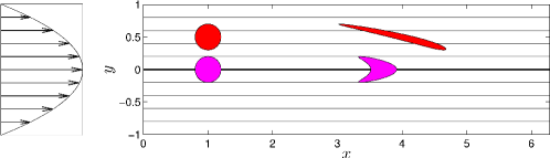
Figure 1: Left: The velocity profile of the steady flow (1) for $u(y)=1-y^{2}$. Right: Streamlines for the same flow. The thick line at $y=0$ marks the shearless streamline that acts as a jet core. The tracer disk located on the shearless line (magenta circle) deforms into a blunt arrow shape symmetrically under advection to time $t=9$. The tracer disk located away from the shearless line (red circle) has a markedly different deformation pattern.

The flow (1) is an idealized model of the velocity field inside atmospheric or oceanic zonal jets, or helical magnetic field lines in a tokamak [1]. As a dynamical system, (1) represents an integrable system with the Hamiltonian $H(y)=\int_{0}^{y}u(\eta)d\eta$. Its horizontal trajectories along which the Eulerian shear $u^{\prime}(y)$ vanishes are referred to as shearless barriers. Along these barriers, $H^{\prime\prime}(y_{0})=0$ holds, thus the circle $y=y_{0}$ does not satisfy the twist condition of classic KAM theory [2].

Yet numerical studies of [13, 31, 35, 38] show that such barriers are more robust under steady or time-periodic perturbations than any other nearby KAM tori. Related theoretical results for two-dimensional maps were given in [17]. More recently, degenerate tori for steady $3$D maps were considered in [37]. In addition, a general a posteriori result on non-twist tori of arbitrary dimension that are potentially far from integrable has been obtained by [23]. However, no general theory of shearless transport barriers for unsteady flows has been established.

The need for such a general theory of unsteady shearless barriers clearly exists. In plasma physics, computational and experimental studies suggest that shearless barriers enhance the confinement of plasma in magnetic fusion devices [27, 29, 28, 9], which generate turbulent velocity fields with general time dependence. In this context, a description of shearless barriers is either understood in models for steady magnetic fields [9] or inferred from scalar quantities (e.g. temperature, density) in more complex unsteady scenarios [27, 29, 28].

In fluid dynamics, shearless barriers are of interest in the context of zonal jets. Rossby waves are the best known and most robust transport barriers in geophysical flows [14, 30, 6], yet only recent work attempts to their attendant unsteady jet cores in the Lagrangian fame of an unsteady flow. The method put forward in [7] seeks such Lagrangian shearless barriers as trenches of the finite-time Lyapunov exponent (FTLE) field. However, just as the examples in [25] show that FTLE ridges do not necessarily correspond to hyperbolic Lagrangian structures, FTLE trenches may also fail to mark zonal jet cores (see Example 1 in Section 7.2 below).

Here we develop a variational principle for shearless barriers as centerpieces of material strips showing no leading order variation in Lagrangian shear. This variational principle shows that shearless barriers are composed of tensorlines of the right Cauchy–Green strain tensor associated with the flow map. Most stretching or contracting Cauchy–Green tensorlines have previously been identified as best candidates for hyperbolic Lagrangian Coherent Structures (LCSs) [26, 20], but no underlying global variational principle has been known to which they would be solutions. The present work, therefore, also advances the theory of hyperbolic LCS, establishing them as shearless transport barriers under fixed (Dirichlet-type) boundary conditions.

Our main result is that parabolic transport barriers (jet cores) are also solutions of the same shearless Lagrangian variational principle, satisfying variable-endpoint boundary conditions. They are formed by minimally hyperbolic, structurally stable chains of tensorlines that connect singularities of the Cauchy–Green strain tensor field. We develop and test a numerical procedure that detects such tensorline chains, thereby finding generalized Lagrangian jet cores in an arbitrary, two-dimensional unsteady flow field in an automated fashion.

2 Notation and definitions

Let $v(x,t)$ denote a two-dimensional velocity field, with $x$ labeling positions in a two-dimensional region $U$, and with $t$ referring to time. Fluid trajectories generated by this velocity field satisfy the differential equation

$$\dot{x}=v(x,t),$$ (2)

whose solutions are denoted by $x(t;t_{0},x_{0}$), with $x_{0}$ referring to the initial position at time $t_{0}$. The evolution of fluid elements is described by the flow map

$$F_{t_{0}}^{t}(x_{0}):=x(t;t_{0},x_{0}),$$ (3)

which takes any initial position $x_{0}$ to its current position at time $t$.

Lagrangian strain in the flow is often characterized by the right Cauchy–Green strain tensor field $C(x_{0})=\left[\nabla F_{t_{0}}^{t}(x_{0})\right]^{T}\nabla F_{t_{0}}^{t}(x_{0})$, whose eigenvalues $\lambda_{i}(x_{0})$ and eigenvectors $\xi_{i}(x_{0})$ satisfy

$$C\xi_{i}=\lambda_{i}\xi_{i},\quad\left|\xi_{i}\right|=1,\quad i=1,2;\qquad 0<\lambda_{1}\leq\lambda_{2},\qquad\xi_{1}\perp\xi_{2}.$$

The tensor $C$, as well as its eigenvalues and eigenvectors, depend on the choice of the times $t$ and $t_{0}$, but we suppress this dependence for notational simplicity.

3 Stability of material lines

Consider a material line (i.e., a smooth curve of initial conditions) $\gamma$ at time $t_{0}$, parametrized as $r(s)$ with $s\in[0,\sigma]$. If $n(s)$ denotes a smoothly varying unit normal vector field along $\gamma$, then the normal repulsion $\rho$ of $\gamma$ over the time interval $[t_{0},t]$ is given by [25]

$$\rho(r,n)=\frac{1}{\sqrt{\left<n,C^{-1}(r)n\right>}},$$ (4)

measuring at time $t$ the normal component of the linearly advected normal vector $\nabla F_{t_{0}}^{t}(r)n$ (see Fig. 2). If $\rho>1$ pointwise along $\gamma$, then the the evolving material line $F_{t_{0}}^{t}(\gamma)$ is repelling. Similarly, if $\rho<1$ holds pointwise along $\gamma$, then the the evolving material line $F_{t_{0}}^{t}(\gamma)$ is attracting.

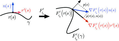
Figure 2: The evolution of a unit normal vector $n(s)$ of a material line $\gamma$ under the linearized flow map $\nabla F_{t_{0}}^{t}$.

Hyperbolic Lagrangian coherent structures (LCSs) are pointwise most repelling or most attracting material lines with respect to small perturbations to their tangent spaces [25, 19, 20]. Repelling and attracting LCSs, respectively, are obtained as special trajectories of the differential equations

$$\dot{r}=\xi_{1}(r),\qquad\dot{r}=\xi_{2}(r),$$ (5)

that stay bounded away from points where $\xi_{i}$ cease to be well-defined. These degenerate points $x_{0}$ are singularities of the Cauchy–Green tensor field, satisfying $C(x_{0})=I$. The trajectories of the differential equations in (5) are called strainlines and stretchlines, respectively [18, 20]. Computing the definition of $\rho$ in (4), we obtain that strainlines repel at a local rate of $\rho(r,n)=\sqrt{\lambda_{2}(r)}$, and stretchlines attract at a rate of $\rho(r,n)=\sqrt{\lambda_{1}(r)}$. Following the terminology used in the scientific visualization community [16, 36], we will refer to strainlines and stretchlines collectively as tensorlines.

A pointwise measure of how close a material curve is to being neutrally stable is the neutrality $\mathcal{N}(r,n)$, defined as

$$\mathcal{N}(r,n)=\left(\rho(r,n)-1\right)^{2}.$$ (6)

Given the explicit normals known for tensorlines, their neutrality can be computed as a sole function of the location $r$, and can be written as

$$\mathcal{N}_{\xi_{1}}(r)=\left(\sqrt{\lambda_{2}(r)}-1\right)^{2},\qquad\mathcal{N}_{\xi_{2}}(r)=\left(\sqrt{\lambda_{1}(r)}-1\right)^{2},$$

respectively, for strainlines and stretchlines.

In this paper, we will be seeking generalized non-twist curves (or jet-cores) that are as close to neutral ($\mathcal{N}\equiv 0$) as possible. Requiring strictly zero neutrality along a material curve $\gamma$ would, however, lead to an overdetermined problem. Indeed, a material line with neutral stability at all its points would be non-generic in an unsteady flow. Instead, we will be interested in material lines that are close to minimizing the neutrality, while also satisfying a minimal-shearing principle to be discussed later.

Here we only work out a close-to-neutral condition for tensorlines, as they will turn out to have special significance in our search for shearless barriers. First, we define the convexity sets $\mathcal{C}_{\xi_{i}}$ of strainlines and stretchlines, respectively, as

$$\mathcal{C}_{\xi_{i}}=\left\{x_{0}\in U:\,\left<\partial_{r}^{2}\mathcal{N}_{\xi_{i}}(x_{0})\xi_{j}(x_{0}),\xi_{j}(x_{0})\right>>0,\qquad i\neq j\right\},\qquad i=1,2.$$

These sets are simply composed of points where the corresponding neutrality is a convex function. We say that a compact tensorline segment $\gamma$ is a weak minimizer of its corresponding neutrality $\mathcal{N}_{\xi_{i}}(r)$ if both $\gamma$ and the nearest trench of $\mathcal{N}_{\xi_{i}}(r)$ lie in the same connected component of $\mathcal{C}_{\xi_{i}}$. More specifically, a weak minimizer $\gamma$ of $\mathcal{N}_{\xi_{i}},$ with parametrization $r_{0}(s)$ and smooth unit normal vector field $n_{0}(s)$, satisfies the condition

$$r_{0}(s)+\epsilon n_{0}(s)\in\mathcal{C}_{\xi_{i}},\qquad s\in[0,\sigma],\quad\epsilon\in[0,\epsilon_{0}(s)],$$ (7)

where

$$\epsilon_{0}(s)=arg\min\left\{\left|\epsilon\right|\in(0,\infty)\,:\,\partial_{\epsilon}\mathcal{N}_{\xi_{i}}\left(r_{0}(s)+\epsilon n_{0}(s)\right)=0,\quad\partial_{\epsilon}^{2}\mathcal{N}_{\xi_{i}}\left(r_{0}(s)+\epsilon n_{0}(s)\right)>0\right\}.$$

4 Eulerian and Lagrangian shear

For the steady two-dimensional steady flow shown in Fig. 1, the classic Eulerian shear in the $x$ direction is defined as the derivative of the horizontal velocity field in the vertical direction, i.e.,

$$\frac{\partial u}{\partial y}=-2y,$$ (8)

which vanishes on the line $y_{0}=0$. This line plays the role of a jet core with a distinguished impact on tracer blobs in comparison to other horizontal streamlines (see Figure 1).

The Eulerian shear, as the normal derivative of a velocity component of interest, can certainly be computed for unsteady flows as well, and is indeed broadly used in fluid mechanics [4]. However, instantaneously shearless curves no longer act as invariant manifolds in the flow, and thus will generally not create the characteristic tracer patterns seen in Fig. 1. As a result, the mathematical description and systematic extraction of jet-core type material barriers in unsteady flows has been an open problem, despite their ubiquitous presence in plasma and geophysics.

To set the stage for a general description of jet-core-type structures, we first need a Lagrangian definition of shear that captures the type of material evolution seen in Fig. 1 even in an unsteady flow. For an arbitrary material curve $\gamma$, we select a parametrization $r(s)$ with $s\in[0,\sigma]$ for $\gamma$ at time $t_{0}$, and with the tangent vectors denoted as $r^{\prime}(s)$.

We denote by $p(s)$ the pointwise tangential shear experienced over the time interval $[t_{0},t]$ along the trajectory starting at time $t_{0}$ from the point $r(s)$. Following [26], we define this tangential shear in the Lagrangian frame as the $\gamma$-tangential projection that a unit vector $n(s)=\left[r^{\prime}(s)\right]^{\perp}$ initially normal to $\gamma$ at $r(s)$ develops by time $t$, as it is advected forward by the linearized flow $\nabla F_{t_{0}}^{t}(r(s))$ (see Fig. 2). Specifically, the Lagrangian shear $p(s)$ is given by

$$p(s) =\left\langle\frac{\nabla F_{t_{0}}^{t}(r(s))r^{\prime}(s)}{\left|\nabla F_{t_{0}}^{t}(r(s))r^{\prime}(s)\right|},\nabla F_{t_{0}}^{t}(r(s))\frac{\left[r^{\prime}(s)\right]^{\perp}}{\left|\left[r^{\prime}(s)\right]^{\perp}\right|}\right\rangle$$

$$=\frac{\left\langle r^{\prime}(s),D(r(s))r^{\prime}(s)\right\rangle}{\sqrt{\left\langle r^{\prime}(s),C(r(s))r^{\prime}(s)\right\rangle\left\langle r^{\prime}(s),r^{\prime}(s)\right\rangle}},$$ (9)

where $\langle\cdot,\cdot\rangle$ denotes the Euclidean inner product, and the tensor field $D$ is defined as

$$D(x_{0})=\frac{1}{2}[C(x_{0})\Omega-\Omega C(x_{0})],\qquad\Omega=\left(\begin{array}[]{cc}0&-1\\ 1&0\end{array}\right).$$ (10)

5 Variational principle for shearless transport barriers

We seek generalized shearless curves as centerpieces of regions with no observable variability in the averaged material shear. Assume that $\epsilon>0$ is a minimal threshold above which we can physically observe differences in material shear over the time interval $[t_{0},t].$ By smooth dependence on initial fluid positions, we will typically observe an $\mathcal{O}(\epsilon)$ variability in shear within an $\mathcal{O}(\epsilon)$-thick strip around a randomly chosen material curve $\gamma$. Our interest, however, is exceptional $\gamma$ curves around which $\mathcal{O}(\epsilon)$-thick coherent strips show no observable variability in their average shearing.

Based on the definition (9), the averaged Lagrangian shear experienced along $\gamma$ over the time interval $[t_{0},t]$ can be written as

$$P(\gamma)=\frac{1}{\sigma}\int_{0}^{\sigma}p(s)\,\mathrm{d}s.$$ (11)

As we argued above, if an observable non-shearing material strip exists around $\gamma$, then on $\epsilon$-close material curves we must have $P(\gamma+\epsilon h)=P(\gamma)+\mathcal{O}(\epsilon^{2}),$ where $\epsilon h(s)$ denotes a small perturbation to $r(s)$. This is only possible if the first variation of $P$ vanishes on $\gamma$:

$$\delta P(\gamma)=0.$$ (12)

This condition leads to the following weak form of the Euler-Lagrange equation:

$$\delta P(\gamma)=\left[\left\langle\partial_{r^{\prime}}p,h\right\rangle\right]_{0}^{\sigma}+\int_{0}^{\sigma}\left[\partial_{r}p-\frac{d}{ds}\partial_{r^{\prime}}p\right]h(s)\,ds=0.$$ (13)

6 Boundary conditions

We are interested in two types of boundary conditions for the variational problem (13):

6.1 Variable endpoint boundary conditions

Variable endpoint boundary conditions mean that $\gamma$ is a stationary curve with respect to all admissible perturbations, i.e., it is the most observable type of centerpiece for shearless coherent strip. As we show in Appendix A, the only possible locations for variable endpoint boundary conditions are those satisfying

$$C\left(r(0)\right)=C\left(r(\sigma)\right)=I.$$ (14)

For completeness, we also consider another variable boundary condition in Appendix A which results in non-zero Lagrangian shear (9) and hence are not discussed here.

6.2 Fixed endpoint boundary conditions

Fixed endpoint boundary conditions mean that $\gamma$ is a stationary curve with respect to all perturbations that leave its endpoints fixed. In this case, we have

$$h(0)=h(\sigma)=0.$$ (15)

These boundary conditions do not place restrictions on the admissible endpoints of $\gamma$. At the same time, a stationary curve under these boundary conditions is generally expected to be less robust or prevalent as a transport barrier than its variable-endpoint counterparts, given that it only prevails as a stationary curve under a smaller class of perturbations.

7 Equivalent geodesic formulation: hyperbolic and parabolic barriers

Under the above two boundary conditions, we obtain from (13) the classic strong form of the Euler–Lagrange equations:

$$\partial_{r}p-\frac{d}{ds}\partial_{r^{\prime}}p=0,$$ (16)

a complicated second-order differential equation for $r(s)$ .

As we show in Appendix B, however, any $\gamma$ satisfying (16) also satisfies

$$\delta\mathcal{P}_{\mu}(\gamma)=0,\qquad\qquad\mathcal{P}_{\mu}(\gamma)=\int_{\gamma}H_{\mu}(r(s),r^{\prime}(s))\,\mathrm{d}s,\qquad H_{\mu}(r(s),r^{\prime}(s))\equiv 0,$$ (17)

and hence represents a zero-energy stationary curve for the shear-energy-type functional

$$H_{\mu}(r,r^{\prime}) =\langle r^{\prime},D(r)r^{\prime}\rangle-\mu\sqrt{\left\langle r^{\prime},C(r)r^{\prime}\right\rangle\left\langle r^{\prime},r^{\prime}\right\rangle}$$ (18)

for some choice of the parameter $\mu$.

Of special interest to us is the case of pointwise shearless curves, which we call perfect shearless barriers. Such barriers should prevail as influential transport barriers at arbitrary small scales. Using the definition of the Lagrangian shear in (9), we conclude that curves with pointwise zero shear within the $H_{\mu}(r(s),r^{\prime}(s))\equiv 0$ energy surface all correspond to the parameter value $\mu=0.$

For this value of $\mu$, zero-energy stationary curves of the functional $\mathcal{P}_{0}(\gamma)$ are null-geodesics of the Lorentzian metric

$$g(u,v)=\langle u,D(x_{0})v\rangle,$$ (20)

which has metric signature $(-,+)$ [5]. The metric $g$ vanishes on its null-geodesics, and hence these null-geodesics satisfy the implicit first-order differential equation

$$\langle r^{\prime}(s),D(r(s))r^{\prime}(s)\rangle\equiv 0.$$ (21)

A direct calculation shows that all solutions of(21) satisfy

$$r^{\prime}(s)\parallel\xi_{i}(r(s)),\qquad i=1\,\,\mathrm{or\,\,2,}$$ (22)

therefore we obtain the following result.

Theorem 1.

Perfect shearless barriers are null-geodesics of the Lorentzian metric $g$, which are in turn composed of tensorlines of the Cauchy–Green strain tensor $C$.

7.1 Hyperbolic barriers

The geodesic transport barrier theory developed in [26] proposed that hyperbolic LCS are individual strainlines and stretchlines that are most closely shadowed by locally most compressing and stretching geodesics, respectively, of the Cauchy–Green strain tensor $C$.

By contrast, here we have obtained from our shearless variational principle (12) that tensorlines of $C$ are null-geodesics for the tensor $D$. Instead of comparing tensorlines to Cauchy–Green geodesics, therefore, one may simply locate hyperbolic LCSs as null-geodesics of $D$ that

H1

stay bounded away from Cauchy–Green singularities (i.e., points where $C=I$), elliptic LCSs (see [26]) and parabolic LCSs (see below).

H2

admit an extremum for the averaged compression or stretching, respectively, among all their neighbors. These averages can be computed by averaging $\sqrt{\lambda_{1}(x_{0})}$ and $\sqrt{\lambda_{2}(x_{0})}$, respectively, along strainlines and stretchlines.

Condition (H1) is required to hold because material curves crossing Cauchy–Green singularities points have zero tangential and normal stretching rates at the singularities, and hence lose their strict normal attraction or repulsion property. It implies that hyperbolic LCSs must satisfy Dirichlet boundary conditions, and none of their interior points can be Cauchy-Green singularities either. As a result, individual hyperbolic LCS are expected to fall in the less robust and prevalent class of shearless barriers, as discussed in Section 6.

Condition (H2) simply implements the definition of LCS as locally most repelling or attracting material curves, reducing an originally infinite-dimensional extremum problem to maximization within a one-dimensional family of strainlines or stretchlines. We summarize the implications of our shearless variational principle for hyperbolic LCS detection.

Proposition 1.

[Hyperbolic LCS as shearless barriers] Hyperbolic LCSs at time $t_{0}$ are null-geodesics of the Lorentzian metric $g$ that are bounded away from $C(x_{0})=I$ singularities of the Cauchy–Greens strain tensor. In addition, repelling LCSs have an average stretching smaller than that of any $C^{1}$ close null-geodesic of $g$ (see Fig. 3 for an illustration). Furthermore, attracting LCSs have an average stretching larger than that of any $C^{1}$ close null-geodesic of $g$.

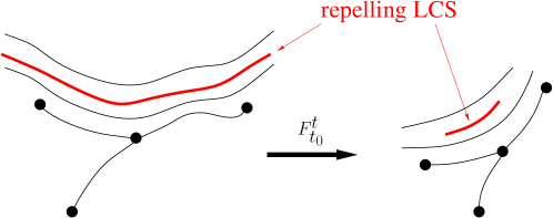
Figure 3: Schematic representation of the properties of a repelling LCS (red) among nearby strainlines (black) and Cauchy–Green singularities (dots). The repelling LCS stays away from singularities of Cauchy–Green singularities. While the length of any strainline shrinks as advected under the flow map $F_{t_{0}}^{t}$, the length of a repelling LCS shrinks more than any $C^{1}$-close strainline.

7.2 Parabolic barriers

Our main focus is to find generalized jet cores in the Lagrangian frame for unsteady flows of arbitrary time dependence. We shall refer to such generalized jet cores here as parabolic transport barriers.

The general solution (22) of our variational principle certainly allows for further types of shearless barriers beyond hyperbolic LCSs. These further barriers are also composed of strainlines and stretchlines, but contain Cauchy–Green singularities and hence fail to be hyperbolic material lines. As discussed in section (6), such non-hyperbolic barriers are the most influential if they satisfy variable-endpoint boundary conditions for our shearless variational principle, i.e., their endpoints are Cauchy–Green singularities.

In addition, in order to provide a generalization of jet cores, we are interested in non-hyperbolic shearless barriers that have no distinct (repelling or attracting) stability type along their interior points. To this end, we require parabolic barriers to be also weak minimizers of their neutrality in the sense of Section 3.

Finally, for reasons of physical relevance and observability, our definition of a parabolic barrier will further restrict our consideration to strainline–stretchline chains that are unique between the two singularities they connect, and are also structurally stable with respect to small perturbations. Based on our review of tensorline singularities in Appendix C, strainlines connecting singularities are only structurally stable and unique if they connect a trisector singularity to a wedge singularity (see Fig. 4). An identical requirement holds for stretchlines.

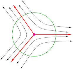
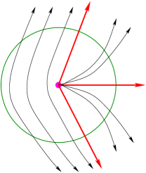
Figure 4: Topology of tensorlines (black) around a trisector (left) and a wedge (right) singularity (magenta). The tensorlines shown in red form the separatrices.

We then have the following definition.

Definition 1.

[Parabolic barriers] Let $\gamma$ denote the time $t_{0}$ position of a compact material line. Then this material line is a parabolic transport barrier over the time interval $[t_{0},t]$ if the following two conditions are satisfied:

P1

$\gamma$ is an alternating chain of strainlines and stretchlines, which is a unique connection between a wedge- and and a trisector-type singularity of the tensor field $C(x_{0})$ (see Fig. 5).

P2

Each strainline and stretchline segment in $\gamma$ is a weak minimizer of its associated neutrality.

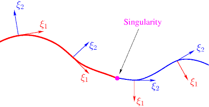
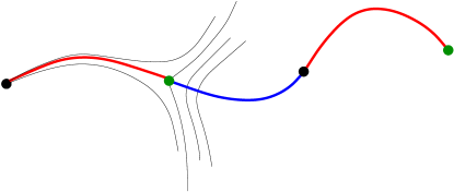
Figure 5: Top: Smooth connection of strainlines (red curve) and stretchlines (blue curve) only occurs at Cauchy–Green singularities. Bottom: An alternating chain of strainlines (red) and stretchlines (blue) connecting trisectors (green) and wedges (black). An schematic phase portrait of strainlines (thin black lines) is shown around one of the trisector singularities. The strainline marked by red color is the unique connection between that trisector and the wedge on its left.

Example 1.

[An FTLE trench is not necessarily a parabolic barrier] Since our notion of a parabolic barrier requires a minimality condition on $\lambda_{2}$, one may speculate whether a trench of the Finite-Time Lyapunov Exponent (FTLE) field will always be a shearless barrier. Such an approach of detecting jet cores by trenches of the combined forward and backward FTLE field was considered in [7]. While the trench of the FTLE field can indeed be an indicator of a jet core, the following example of a steady two-dimensional incompressible flow shows that this is not necessarily the case. Consider the incompressible flow

$$\begin{split}&\dot{x}=x\left(1+3y^{2}\right),\\ &\dot{y}=-y-y^{3}.\end{split}$$ (23)

The line $y=0$ is an invariant, attracting set, yet numerical simulations show that it is also a trench of the FTLE field, as seen in Figure 6. The figure also shows by tracer advection that this trench is a hyperbolic (attracting) LCS, as opposed to a parabolic barrier acting as a jet core.

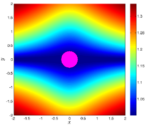
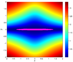
Figure 6: The tracer evolution for system (23). Left: Initial circular blob of tracers centered at the origin at time $t=0$. Right: The advected tracer at time $t=1.5$. The forward-time FTLE field with integration time $T=10$ is shown in the background.

8 Automated numerical detection of parabolic barriers

Definition 1 provides the basis for the identification of parabolic barriers in finite-time flow data. Using the numerical details surveyed in Appendix C, we implement conditions P1 and P2 of Definition 1 as follows:

1. Compute the Cauchy–Green strain tensor $C$ on a two-dimensional grid in the $(x_{1},x_{2})$ variables.

2. Detect the singularities of $C$ by finding the common zeros of $f=C_{11}-C_{22}$ and $g=C_{12}$.

3. For any trisector singularity of the $\xi_{1}$ vector field, follow strainlines emanating from the singularity and identify among them the separatrices connecting the trisectors to wedges. Repeat the same procedure for the $\xi_{2}$ vector field to find trisector-wedge separatrices among stretchlines.

4. Out of the computed separatrices, keep the strainline separatrices satisfying $\left<\partial_{r}^{2}\mathcal{N}_{\xi_{1}}(x_{0})\xi_{2}(x_{0}),\xi_{2}(x_{0})\right>>0$, and the stretchline separatrices satisfying $\left<\partial_{r}^{2}\mathcal{N}_{\xi_{2}}(x_{0})\xi_{1}(x_{0}),\xi_{1}(x_{0})\right>>0$.

5. Build smoothly connecting, alternating stretchline-strainline heteroclinic chains form the separatrices so obtained.

6. Finally, keep only the heteroclinic chains whose individual components are weak minimizers of their neutralities.

9 Numerical examples

9.1 Standard non-twist map

We first consider the standard non-twist map (SNTM)

$$\begin{split}&x_{n+1}=x_{n}+a\left(1-y_{n+1}^{2}\right),\\ &y_{n+1}=y_{n}-b\sin(2\pi x_{n}),\end{split}$$ (24)

which was first studied in detail in [13], and has since become a generally helpful model in understanding shearless KAM curves in two-dimensional steady or temporally periodic incompressible flows.

For $b=0$, the map (24) is a discretized version of the canonical parallel shear flow (1) with vanishing Eulerian shear along $y=0$. For steady perturbations of (1), one still has a steady streamfunction whose dynamics is integrable and the shearless barriers can be understood as the lack of Hamiltonian twist. For $b\neq 0$, the SNTM corresponds to the evolution of a time-periodic perturbation of (1).

For the parameter values $a=0.08$, $b=0.125$, the SNTM is integrable and well-understood. We choose these parameters to illustrate the performance of our theory and extraction methodology for parabolic barriers. Figure 7a shows the orbits of SNTM for these integrable parameters.

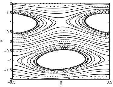
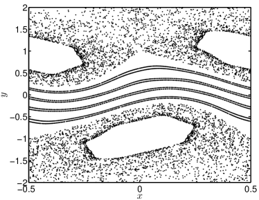
Figure 7: The standard non-twist map. Left: Integrable parameters: $a=0.08$, $b=0.125$ Right: Chaotic parameters: $a=0.27$, $b=0.38$.

In this integrable case, the location of shearless barriers is no longer trivial, but can be found by the theory of indicator points [33]. Specifically, initial conditions for the shearless barrier are given by

$$x=\pm\left(\frac{a}{2}+\frac{1}{4}\right)\ \ \mbox{and}\ \ y=0,$$ (25)

and the full barrier can be constructed by iterating these initial condition under the map (24). Therefore, we can compare the parabolic barrier computed from finitely many iterations using the steps in Section 8 with the exact asymptotic shearless barrier of the map.

Figure 8 shows all heteroclinic tensorlines connecting trisectors to wedges (left panel). In the domain $[-0.5,0.5]\times[-2,2]$ and for $100$ iterations of the SNTM, we find $6$ singularities: 2 trisectors (green dots) and 4 wedges (black dots). Only 4 alternating sequence of tensorlines satisfy conditions P1 and P2 of Definition 1. Figure 8 also shows the extracted parabolic barrier, i.e., a heteroclinic chain formed by four tensorlines (note the periodicity in $x$). This parabolic barrier represents the finite-time version of the exactly known asymptotic shearless KAM curve.

One can also compute the parabolic barrier for higher iterations of the SNTM map with the same procedure. As the number of iterations increase, the computed parabolic barrier converges to the exact asymptotic barrier. In Fig. 9, we show this convergence up to $300$ iterations. For higher iterations, the two barriers become practically indistinguishable. The exact barrier (black curve) in Fig. 9 is computed from $200$ iterations of the indicator points (25).

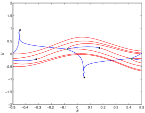
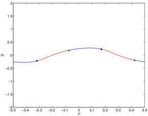
Figure 8: Left: Heteroclinic tensorlines between trisector and wedge singularities of the Cauchy–Green strain tensor in the integrable SNTM: strainlines (red) and stretchlines (blue). The black and green dots mark the wedge and trisector singularities, respectively. Right: The extracted parabolic barrier consists of the single alternating sequence of tensorlines that satisfy conditions P1-P2 of Definition 1.

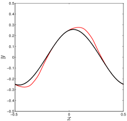
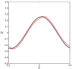
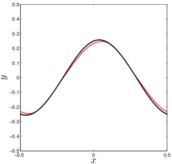
Figure 9: The red curve shows the computed finite-time shearless barrier from $100$ (left), $200$ (middle) and $300$ (right) iterations of the integrable SNTM with parameters $a=0.08$ and $b=0.125$. The black curve marks the exact location of the barrier.

The evolution of circular tracers off and on the computed parabolic barriers is shown in Fig. 10 The purple tracer in the left plot of Fig. 10 is located on the computed parabolic barrier (red). The magenta and green tracers are centered on a tensorline (blue) that does not satisfy condition P2 of Definition 1. The images of all the tracers after $100$ iterations of SNTM are shown in the right panel of Fig. 10. While the purple tracer undergoes a small boomerang-like deformation expected along parabolic barriers (jet cores), the other two tracer blobs experience substantial stretching. This illustrates that condition P2 is indeed essential in identifying parabolic barriers.

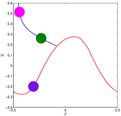
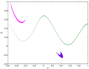
Figure 10: Parabolic barrier and its impact on tracers in the integrable SNTM.

The SNTM (24) becomes chaotic for parameters $a=0.27$, $b=0.38$. The theory of indicator points still applies and gives the exact asymptotic barrier for comparison. Figure 11 compares the computed parabolic barrier with the asymptotic shearless barrier. The parabolic barrier is constructed from $100$ iterations of the SNTM while the exact barrier is computed from $200$ iterations of the indicator point.

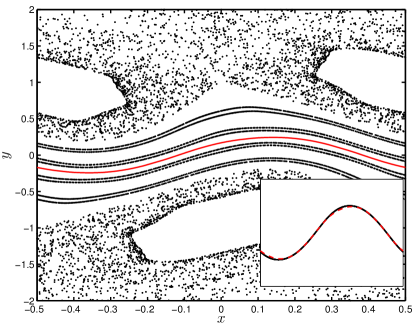
Figure 11: The chaotic SNTM with parameters $a=0.27$, $b=0.38$. The red curve shows the parabolic barrier computed from $100$ iterations of SNTM. The inset compares the parabolic barriers with the exact asymptotic barrier (black curve) obtained by $200$ iterations of the indicator points.

9.2 Passive particles in mean-field coupled non-twist maps

Following [12, 11], we consider the self-consistent mean field interaction of $N$ coupled standard non-twist maps

$$\begin{split}&x_{n+1}^{k}=x_{n}^{k}+a\left(1-\left(y_{n+1}^{k}\right)^{2}\right),\\ &y_{n+1}^{k}=y_{n}^{k}-b_{n+1}\sin(2\pi x_{n}^{k}-\theta_{n}),\end{split}$$ (26)

where $k=1,\ldots,N$ is an index for the particles and $n$ is the iteration number. The variables $\theta_{n}$ and $b_{n}$ are given by

$$\begin{split}&\theta_{n+1}=\theta_{n}+\frac{1}{b_{n+1}}\frac{\partial\eta_{n}}{\partial\theta_{n}},\\ &b_{n+1}=\sqrt{\left(b_{n}\right)^{2}+\left(\eta_{n}\right)^{2}}+\eta_{n},\end{split}$$ (27)

where

$$\eta_{n}=\sum_{i=1}^{n}\gamma_{i}\sin\left(x_{n}^{i}-\theta_{n}\right).$$ (28)

We refer to the particles $x_{n}^{i}$ as active particles since they influence the mean field. The coefficients $\gamma_{i}$ are the coupling constants. The mean field model (26)-(27) arises from studying vorticity defects in perturbations of parallel shear flow [12, 3], and also has applications in one-dimensional beam plasmas [34, 12].

The full mean-field system is $2N$-dimensional, and we consider the behavior of a passive particle, whose non-autonomous evolution is given by

$$\begin{split}&x_{n+1}=x_{n}+a\left(1-y_{n+1}^{2}\right),\\ &y_{n+1}=y_{n}-b_{n+1}\sin(2\pi x_{n}-\theta_{n}),\end{split}$$ (29)

where $b_{n}$ and $\theta_{n}$ are determined by the mean field of active particles. The evolution of a passive particle is similar to that of the SNTM considered in Section 9.1, but the parameters $b_{n}$ and $\theta_{n}$ change under each iteration according to the mean field interaction of the active particles. When the coupling constants $\gamma_{i}$ are zero, system (29) coincides with the autonomous SNTM (24).

We take $a=0.08$ and $b_{0}=0.125$ and $\theta_{0}=0.0$. The corresponding dynamics for the SNTM (24) are integrable as described in the previous section. With these initial parameters, we place $N=2\times 10^{4}$ active particles localized near the islands (see Fig. 12) and compute their mean field evolution. The coupling constants $\gamma_{i}$ are $2\times 10^{-5}$ for all $i$. The evolution of the parameter $b_{n}$ is shown in Figure 12, and one thus sees that the evolution of a passive particle is aperiodic with respect to the iteration number.

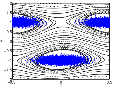
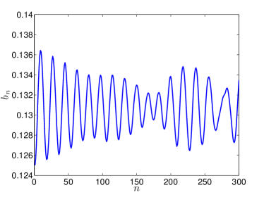
Figure 12: Left: Initial conditions of the active particles. Right: Aperiodic evolution of $b_{n}$.

With this setting, we compute all heteroclinic tensorlines using the automated algorithm described in Section 8. Shown in the left plot of Figure 13, the extracted heteroclinic tensorline geometry is more complicated than what we found for the SNTM. However, as seen in the right-side plot of the figure, the final subset of connections satisfying conditions P1-P2 of Definition 1 is similar to that of the integrable system. This implies the persistence of a parabolic shearless barrier for a passive tracer in a self-consistent mean-field model.

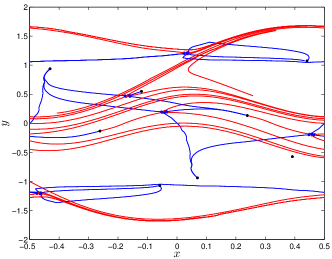
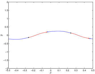
Figure 13: Left: Tensorlines for passive tracers in (29) strainlines (red) and stretchlines (blue). The black dots mark the wedge singularities where the tensorlines end. Right: Parabolic barrier as an alternating sequence of tensorlines satisfying conditions P1-P2 of Definition 1.

The evolution of tracers around the parabolic barrier is similar to that shown in Figure 10. Instead of presenting the tracer evolution, however, we illustrate the role of the parabolic barrier by placing two horizontal lines of particles above and two below the parabolic barrier (cf. left plot of Fig. 14). The middle and right plots in the same figure show the advected images of these lines after $50$ and $100$ iterations, respectively. We conclude that despite the generally chaotic mixing prevalent in the map, the extracted parabolic barrier provides a sharp and coherent dividing surface that inhibits transport of passive particles.

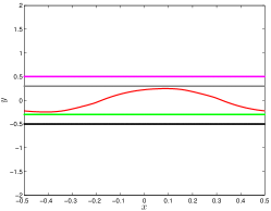
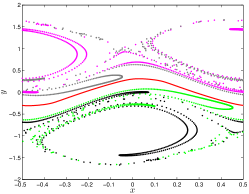
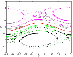
Figure 14: Left: Parabolic barrier (red) and tracer particles (straight lines) at the initial time. Advected images of the parabolic barrier and tracer particles are shown after $50$ iterations (middle) and a $100$ iterations (right)

9.3 Bickley jet

As our last example, we consider an idealized model of an eastward zonal jet known as the Bickley jet [14, 30] in geophysical fluid dynamics. This model consists of a steady background flow subject to a time-dependent perturbation. The time-dependent Hamiltonian for this model reads

$$\psi(x,y,t)=\psi_{0}(y)+\psi_{1}(x,y,t),$$ (30)

where

$$\psi_{0}(y)=-UL\tanh\left(\frac{y}{L}\right),$$ (31)

is the steady background flow and

$$\psi_{1}(x,y,t)=UL\mathrm{sech}^{2}\left(\frac{y}{L}\right)\mbox{Re}\left[\sum_{n=1}^{3}f_{n}(t)\exp(\mbox{i}k_{n}x)\right],$$ (32)

is the perturbation. The constants $U$ and $L$ are characteristic velocity and characteristic length scale, respectively. For the following analysis, we apply the set of parameters used in [30]:

$$U=62.66\;\mbox{ms}^{-1},\ \ L=1770\;\mbox{km},\ \ k_{n}=2n/r_{0},$$ (33)

where $r_{0}=6371\;\mbox{km}$ is the mean radius of the earth.

9.3.1 Quasiperiodic Bickley jet

For $f_{n}(t)=\epsilon_{n}\exp(-\mbox{i}k_{n}c_{n}t)$, the time-dependent part of the Hamiltonian consists of three Rossby waves with wave-numbers $k_{n}$ traveling at speeds $c_{n}$. The amplitude of each Rossby wave is determined by the parameters $\epsilon_{n}$. For small constant values of parameters $\epsilon_{n}$, the Bickley jet is known to have a closed, shearless jet core. In [7], it is shown numerically that this jet core is marked by a trench of the forward- and backward-time FTLE fields. This finding is a consequence of temporal quasi-periodicity of Rossby waves, which renders the the forward- and backward-time dynamics as similar. In general, however, the time-dependence $f_{n}(t)$ can be any smooth signal [26] with no particular recurrence. We focus here on the existence of the shearless jet core under such general forcing functions.

First, however, we compare our results with those of [7] for the quasi-periodic forcing $f_{n}(t)=\epsilon_{n}\exp(-\mbox{i}k_{n}c_{n}t)$, with constant amplitudes $\epsilon_{1}=0.075$, $\epsilon_{2}=0.4$ and $\epsilon_{3}=0.3$. The top plot of Fig. 15 shows automatically extracted heteroclinic tensorlines initiated from trisectors and ending in wedges. Out of all these connections, three satisfy conditions P1-P2 of Definition 1 and hence qualify as parabolic barriers (bottom plot of Fig. 15).

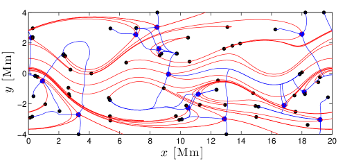
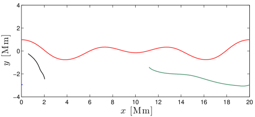
Figure 15: Top: Tensorlines for the quasi-periodically forced Bickley jet: strainlines (red) and stretchlines (blue). The black dots mark the wedge singularities where the tensorlines end in while the blue dots mark the trisectors where the tensorlines are initiated from. Bottom: Automatically extracted parabolic barriers in the quasiperiodic Bickley jet.

The closed ($x$-periodic) parabolic barrier in red has also been obtained in [7] as a trench of both the forward and the backward FTLE field. The other two open parabolic barriers (blue and black), however, have remained undetected in previous studies to the best of our knowledge. Yet these open parabolic barriers do serve as cores of smaller-scale jets, as demonstrated by the distinct boomerang-shaped patterns developed by tracer blobs initialized along them (see Fig. 16).

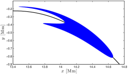
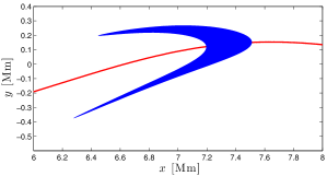
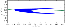
Figure 16: The deformation of initially circular tracers (of radii $0.2$ Mm) centered on the shearless curves after $11$ days. The color of the curves correspond to those of Fig. 15.

Such shearless material curves do not exist in the steady or time-periodic counterpart of the Bickley jet, and thus perturbative theories, such at KAM-type arguments, would not predict the existence of such a jet core. Moreover, since these curves are not closed barriers separating the phase space they cannot be detected as almost-invariant coherent sets [21].

9.3.2 Chaotically forced Bickley jet

To generate chaotic forcing for the Bickley jet, we let the forcing amplitudes $\epsilon_{n}$ to be a chaotic signal for $n=1,2$. The forcing amplitude $\epsilon_{3}=0.3$ remains constant. Figure 17, shows the chaotic signals $\epsilon_{1}(t)$ and $\epsilon_{2}(t)$.

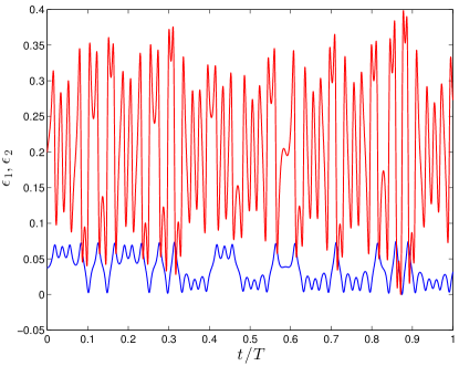
Figure 17: The chaotic signals $\epsilon_{1}$ (blue) and $\epsilon_{2}$ (red) used as the amplitude of the forcing in equation (32). The integration time $T$ is 11 days.

Figure 18 shows the single parabolic barrier obtained from the automated extraction procedure described in Section 8. The additional open parabolic barriers found in the quasi-periodically forced case are, therefore, destroyed under chaotic forcing.

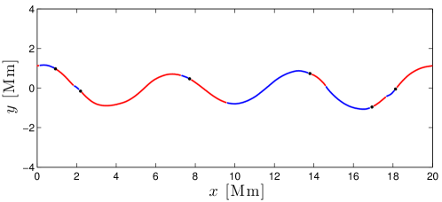
Figure 18: The shearless curve for chaotically forced Bickley jet. The shearless curve consists of alternating sequence of strainlines (red) and stretchlines (blue). The wedge singularities are marked by black dots.

The dynamic role of the remaining single barrier is illustrated in Fig. 19, where initially straight lines of passive particles are advected for $6$, $9$ and $11$ days. Despite widespread chaotic mixing, the parabolic barrier preserves its coherence, showing no stretching, folding, or smaller-scale filamentation. Therefore, the extracted parabolic barrier is a sharp separator between two invariant mixing regions. This shows that beyond the almost-invariant sets located for the Bickley jet by set-theoretical methods [15, 21], actual invariant sets with sharp, coherent boundaries also exist for the parameter values considered here.

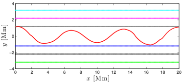
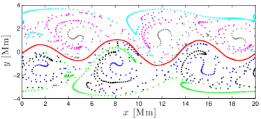
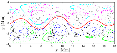
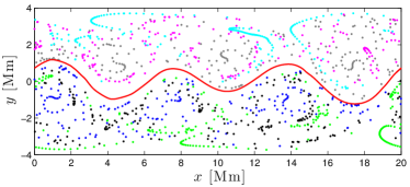
Figure 19: Chaotically forced Bickley jet. The closed shearless curve (red) and tracer particles (dots) at time $t=0$ (top left). Their advected images are shown after 6 days (top right) 9 days (bottom left) and 11 days (bottom right).

10 Conclusions

We have developed a variational principle for shearless material lines in two-dimensional, non-autonomous dynamical systems. Solutions to this principle turn out to be composed of tensorlines of the Cauchy–Green strain tensor. Locally most stretching or contracting tensorlines staying away from singularities of the Cauchy–Green strain tensor are found to be hyperbolic Lagrangian Coherent Structures (LCSs). Thus, the present results give the first global variational description of hyperbolic LCS as shearless material curves.

By contrast, special chains of alternating tensorlines between Cauchy–Green singularities define another class of shearless barriers, which we call parabolic barriers (or parabolic LCSs). These barriers satisfy variable-endpoint boundary conditions in the underlying Euler-Lagrange equation, which make them exceptionally robust with respect to a broad class of perturbations. This explains the broadly reported robustness of shearless barriers observed in physical systems.

We have devised an algorithm for the automated numerical detection of parabolic barriers in two-dimensional unsteady flows. We illustrated this algorithm on the standard non-twist map (SNTM), passive tracers in mean-field coupled SNTMs and a model of the zonal jet (known as the Bickley jet). For the SNTM, we showed that under increasing iterations, our parabolic barrier converges to the exact shearless curve predicted by the theory of indicator points.

For the Bickley jet, we have recovered the results of [7] on closed zonal jet cores under quasi-periodic forcing. We have also found, however, other open jet cores in the same setting that were not revealed by previous studies. A zonal jet was also detected in a chaotically forced Bickley jet.

While higher-dimensional shearless barriers have not yet been studied extensively, the variational methods developed here should extend to higher-dimensional flows. Such an extension of the concept of a parabolic barrier appears to be possible via the approach developed recently for elliptic and hyperbolic transport barriers in three-dimensional unsteady flows [10].

Appendix A Derivation of variable-endpoint boundary conditions for the shearless variational principle

Note that

$$\partial_{r^{\prime}}p = \frac{\left[2\left\langle r^{\prime},Cr^{\prime}\right\rangle\left\langle r^{\prime},r^{\prime}\right\rangle D-\left\langle r^{\prime},Dr^{\prime}\right\rangle\left\langle r^{\prime},r^{\prime}\right\rangle C-\left\langle r^{\prime},Dr^{\prime}\right\rangle\left\langle r^{\prime},Cr^{\prime}\right\rangle I\right]r^{\prime}}{\sqrt{\left\langle r^{\prime},Cr^{\prime}\right\rangle\left\langle r^{\prime},r^{\prime}\right\rangle}^{3}}$$ (34)

Defining

$$M:=\frac{2\left\langle r^{\prime},Cr^{\prime}\right\rangle\left\langle r^{\prime},r^{\prime}\right\rangle D-\left\langle r^{\prime},Dr^{\prime}\right\rangle\left\langle r^{\prime},r^{\prime}\right\rangle C-\left\langle r^{\prime},Dr^{\prime}\right\rangle\left\langle r^{\prime},Cr^{\prime}\right\rangle I}{\sqrt{\left\langle r^{\prime},Cr^{\prime}\right\rangle\left\langle r^{\prime},r^{\prime}\right\rangle}^{3}},$$

we have

$$\partial_{r^{\prime}}p=Mr^{\prime}.$$ (35)

Any perturbation $h$ can be written as $h=h_{\parallel}+h_{\perp}$ where $h_{\parallel}$ and $h_{\perp}$ are, respectively, the tangential and orthogonal components of $h$ with respect to $r^{\prime}$. Therefore, the boundary term in (13) can be written as

$$\langle\partial_{r^{\prime}}p,h\rangle=\langle Mr^{\prime},h_{\perp}\rangle.$$ (36)

Note that the term $\langle Mr^{\prime},h_{\parallel}\rangle$ vanishes since $\langle Mr^{\prime},r^{\prime}\rangle=0$.

Since $h_{\perp}$ is a scalar multiple of $\Omega r^{\prime}$, the boundary term $\langle\partial_{r^{\prime}}p,h\rangle$ vanishes if and only if $\langle Mr^{\prime},\Omega r^{\prime}\rangle=0$. Now expanding $r^{\prime}$ in the Cauchy–Green eigenbasis as $r^{\prime}=\alpha\xi_{1}+\beta\xi_{2}$, we get

$$\langle Mr^{\prime},\Omega r^{\prime}\rangle=\frac{(\alpha^{2}\lambda_{1}+\beta^{2}\lambda_{2})(\alpha^{2}-\beta^{2})(\lambda_{2}-\lambda_{1})-\alpha^{2}\beta^{2}(\lambda_{2}-\lambda_{1})^{2}}{(\alpha^{2}+\beta^{2})^{1/2}(\alpha^{2}\lambda_{1}+\beta^{2}\lambda_{2})^{3/2}},$$ (37)

where we used the fact that $C\xi_{i}=\lambda_{i}\xi_{i}$ for $i=1,2$. Without loss of generality, we may assume that the tangent vector $r^{\prime}$ is normalized such that $\alpha^{2}+\beta^{2}=1$.

Clearly if $\lambda_{2}=\lambda_{1}$, $\langle Mr^{\prime},\Omega r^{\prime}\rangle$ vanishes and so does the boundary term $\langle\partial_{r^{\prime}}p,h\rangle$. By definition, the eigenvalues $\lambda_{1}$ and $\lambda_{2}$ only coincide at the Cauchy–Green singularities. For an incompressible flow, $C=I$ at the Cauchy–Green singularities since $\lambda_{1}\lambda_{2}=1$. This proves the condition (14).

Alternatively, assuming $\lambda_{1}\neq\lambda_{2}$, we find that $\langle Mr^{\prime},\Omega r^{\prime}\rangle=0$ if and only if

$$\alpha=\pm\sqrt{\frac{\sqrt{\lambda_{2}}}{\sqrt{\lambda_{1}}+\sqrt{\lambda_{2}}}},\ \ \ \beta=\pm\sqrt{\frac{\sqrt{\lambda_{1}}}{\sqrt{\lambda_{1}}+\sqrt{\lambda_{2}}}}.$$

In other words, for the boundary term $\langle\partial_{r^{\prime}}p,h\rangle$ to vanish, the tangent vectors $r^{\prime}$ at the endpoints of $\gamma$ must satisfy

$$r^{\prime}=\sqrt{\frac{\sqrt{\lambda_{2}}}{\sqrt{\lambda_{1}}+\sqrt{\lambda_{2}}}}\;\xi_{1}\pm\sqrt{\frac{\sqrt{\lambda_{1}}}{\sqrt{\lambda_{1}}+\sqrt{\lambda_{2}}}}\;\xi_{2}.$$

The above linear combination of the Cauchy–Green eigenvectors is referred to as the shear vector field [26]. Shearlines, i.e. the solution curves of the shear vector field, have been shown to mark boundaries of coherent regions of the phase space [26, 24, 8], e.g., generalized KAM tori and coherent eddy boundaries.

Shear vector fields, however, do not result in shearless transport barriers; in fact, they are local maximizers of Lagrangian shear [26].

Appendix B Equivalent formulation of the shearless variational principle

With the shorthand notation

$$A(r,r^{\prime})=\langle r^{\prime},C(r)r^{\prime}\rangle,\quad B(r^{\prime})=\langle r^{\prime},r^{\prime}\rangle,\quad G(r,r^{\prime})=\langle r^{\prime},D(r)r^{\prime}\rangle,$$ (38)

$P$ can be rewritten as

$$P(\gamma)=\frac{1}{\sigma}\int_{0}^{\sigma}p(r,r^{\prime})\,\mathrm{d}s=\frac{1}{\sigma}\int_{0}^{\sigma}\frac{G(r,r^{\prime})}{\sqrt{A(r,r^{\prime})B(r^{\prime})}}\,\mathrm{d}s,$$ (39)

and its Euler–Lagrange equations (16) can be re-written as

$$\partial_{r}\frac{G}{\sqrt{AB}}-\frac{d}{\mathrm{d}s}\partial_{r^{\prime}}\frac{G}{\sqrt{AB}}=0.$$ (40)

Note that

$$\partial_{r}\frac{G}{\sqrt{AB}}=\frac{\partial_{r}G}{\sqrt{AB}}-\frac{G\left(B\partial_{r}A+A\partial_{r}B\right)}{2\sqrt{AB}^{3}},\quad\partial_{r^{\prime}}\frac{G}{\sqrt{AB}}=\frac{\partial_{r^{\prime}}G}{\sqrt{AB}}-\frac{G\left(B\partial_{r^{\prime}}A+A\partial_{r^{\prime}}B\right)}{2\sqrt{AB}^{3}},.$$ (41)

Since the integrand of $P(\gamma)$ has no explicit dependence on the parameter $s$, Noether’s theorem [22] guarantees the existence of a first integral for (40). This integral can be computed as

$$I=\frac{G}{\sqrt{AB}}-\left\langle r^{\prime},\partial_{r^{\prime}}\frac{G}{\sqrt{AB}}\right\rangle=\frac{G}{\sqrt{AB}}=I_{0}=\mathrm{const},$$ (42)

where we have used the specific form of the functions $A$ and $B$ from (38), as well as the second equation from (41).

With the notation $\mu=I_{0}$ , we therefore have the identity

$$G(r(s),r^{\prime}(s))\equiv\mu\sqrt{A(r(s),r^{\prime}(s))B(r^{\prime}(s))}$$ (43)

on any solution (40) for some appropriate value of the positive constant $\mu>0$ .

We use the identity (43) to rewrite the expressions (41) as

$$\partial_{r}\frac{G}{\sqrt{AB}}=\frac{1}{\sqrt{AB}}\partial_{r}\left[G-\mu\sqrt{AB}\right],\quad\partial_{r^{\prime}}\frac{G}{\sqrt{AB}}=\frac{1}{\sqrt{AB}}\partial_{r^{\prime}}\left[G-\mu\sqrt{AB}\right].$$ (44)

We also introduce a rescaling of the independent variable $s$ in equation (40) via the formula

$$\frac{\mathrm{d}\tau}{\mathrm{d}s}=\sqrt{A(r(s),r^{\prime}(s))B(r^{\prime}(s))},$$ (45)

which, by the chain rule, implies

$$\sqrt{A(r(s),r^{\prime}(s))B(r^{\prime}(s))}=\frac{1}{\sqrt{A(r(\tau),\dot{r}(\tau))B(\dot{r}(\tau))}},$$ (46)

with the dot referring to differentiation with respect to the new variable $\tau$. Note that $\sqrt{A(r(s),r^{\prime}(s))B(r^{\prime}(s))}$ is non-vanishing on smooth curves with well-defined tangent vectors, and hence the change of variables (45) is well-defined.

After the $s\mapsto\tau$ rescaling and the application of (46), the expressions in (44) imply

$$\partial_{r}\frac{G(r,r^{\prime})}{\sqrt{A(r,r^{\prime})B(r^{\prime})}} = \frac{\partial_{r}\left[G(r,\dot{r})-\mu\sqrt{A(r,\dot{r})B(\dot{r})}\right]}{\sqrt{A(r(\tau),\dot{r}(\tau))B(\dot{r}(\tau))}}$$

$$\frac{\mathrm{d}}{\mathrm{d}s}\partial_{r^{\prime}}\frac{G(r,r^{\prime})}{\sqrt{A(r,r^{\prime})B(r^{\prime})}} = \frac{\frac{\mathrm{d}}{\mathrm{d}\tau}\partial_{\dot{r}}\left[G(r,\dot{r})-\mu\sqrt{A(r,\dot{r})B(\dot{r})}\right]}{\sqrt{A(r(\tau),\dot{r}(\tau))B(\dot{r}(\tau))}}.$$

Based on these identities, equation (40) can be re-written as

$$\frac{1}{\sqrt{A(r(\tau),\dot{r}(\tau))B(\dot{r}(\tau))}}\left\{\partial_{r}\left[G(r,\dot{r})-\mu\sqrt{A(r,\dot{r})B(\dot{r})}\right]-\frac{\mathrm{d}}{\mathrm{d}\tau}\partial_{\dot{r}}\left[G(r,\dot{r})-\mu\sqrt{A(r,\dot{r})B(\dot{r})}\right]\right\}=0.$$ (49)

Since $1/\sqrt{A(r(\tau),\dot{r}(\tau))B(\dot{r}(\tau))}$ is non-vanishing we obtain from (49) that all solutions of (40) must satisfy the Euler–Lagrange equation derived from the Lagrangian

$$\mathcal{H}_{\mu}(r,\dot{r})=\frac{1}{2}\left[G(r,\dot{r})-\mu\sqrt{A(r,\dot{r})B(\dot{r})}\right].$$ (50)

Therefore, all stationary functions of the functional $P$ are also stationary functions of the function for an appropriate value of $\mu$. This value of $\mu$ can be determined from formula (43), which also shows that the corresponding stationary functions of $\mathcal{H}_{\mu}$ all satisfy

$$\langle\dot{r}(\tau),D(r(\tau))\dot{r}(\tau)\rangle=\mu\sqrt{A(r,\dot{r})B(\dot{r})}.$$ (51)

For $\mu=0$, these solutions are null-geodesics of the Lorentzian metric (20) induced by the tensor $D$.

Conversely, assume that $r(\tau)$ satisfies both equations (49) and (51). Reversing the steps leading to (51), and employing the inverse rescaling of the independent variable as,

$$\frac{\mathrm{d}s}{\mathrm{d}\tau}=\sqrt{A(r(\tau),\dot{r}(\tau))B(\dot{r}(\tau))},$$ (52)

we obtain that any rescaled solution $r(s)$ is also a solution of the Euler–Lagrange equation (40). Therefore, each solution of (49) lying in the zero energy surface $\mathcal{H}_{\mu}(r,\dot{r})=0$ is also a stationary curve of the functional $P(\gamma)$, lying on the energy surface $I(r,r^{\prime})=\mu$, and hence satisfying the identity (43).

Appendix C Tensorline singularities, heteroclinic tensorlines, and their numerical detection

Here we briefly review some relevant aspects of tensorline geometry near singularities of a symmetric tensor field [16, 36].

C.1 Tensorline singularities

Singularities of tensorlines, such as the tensorlines of the Cauchy–Green strain tensor, are points where the tensor field becomes the identity tensor, and hence ceases to admit a well-defined pair of eigenvectors. As a consequence, tensorlines, as curves tangent to $\xi_{1}$ and $\xi_{2}$ eigenvector fields, are no longer defined at singularities. Still, the behavior of tensorlines near a singularity has some analogies, as well as notable differences, with the behavior of trajectories of a two-dimensional vector field near fixed point. In the absence of symmetries, there are two structurally stable singularities of a tensorline field: trisectors and wedges.

Trisector singularities are similar to saddle points in two-dimensional flows, except that they have three (as opposed to two) distinguished strainlines asymptotic to them (Fig. 4).

Wedge singularities are a mix between a saddle and a source or a sink. On the one hand, there is a continuous family of infinitely many neighboring tensorlines asymptotic to a wedge. At the same time, a wedge also has discrete tensorlines asymptotic to it, resembling the stable and unstable manifolds of a saddle (Fig. 4).

C.2 Numerical detection of singularities

At a singularity in an incompressible flow, the elements of the Cauchy–Green strain tensor satisfy

$$C_{11}-C_{22}=0\ \ \mbox{and}\ \ C_{12}=0,$$ (53)

where $C_{ij}$ is the $(i$,$j)$ the entry of $C$. The singularities are, therefore, precisely points where the zero level-curves of the scalar functions $f=C_{11}-C_{22}$ and $g=C_{12}$ intersect. These intersections can be found by linearly interpolating $f$ and $g$ along the edges of a numerical grid [16].

In regions of high mixing and chaos, the entries of the Cauchy–Green strain tensor can be large and noisy. An indication of noise in an incompressible flow is that the determinant of $C$ is far from being equal to $1$. These noisy points result in spurious intersection of the zero levels of $f$ and $g$, and hence spurious singularity detection.

A crude but effective way of filtering out most if the these spurious intersections is to consider only parts of the zero level set of $f$ and $g$ on which $|\lambda_{1}\lambda_{2}-1|>1$ holds.

C.3 Numerical classification of singularities

Once the singularities are located, we need a robust procedure to classify each of these singularities as a wedge or a trisector. The existing methods for distinguishing trisector singularities of a tensor field from its wedge singularities require further differentiation of the tensor field [36]. In our experience, this introduces further noise affecting the robustness of the results. Here, we introduce a differentiation-free method for identifying trisectors and wedges. This method also is used to find the direction of the separatrices emanating from a trisector.

A distinguishing geometric feature of a trisector singularity is the three separatrices emanating from it. Close enough to the singularity, these separatrices are close to straight lines. Therefore, the separatrices will be approximately perpendicular to a small circle centered at the singularity. Consequently. the intersection of the trisectors with the circle approximately maximizes the quantity

$$f_{i}(\theta)=\frac{|\left<\xi_{i},r\right>|}{\left|\xi_{i}\right|\left|r\right|}$$ (54)

associated with the vector field $\xi_{i}$, with $r$ is the vector from the singularity pointing towards the point $\theta$ on the small circle.

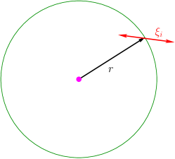
Figure 20: In equation (54), $f(\theta)$ is defined as the normalized inner product of $r$ and $\xi_{i}$.

For a trisector, $f_{i}(\theta)$ assumes the value $0$ and $1$ three times, with $0$’s and $1$’s alternating, as $\theta$ increases from $0$ to $2\pi$. In contrast, for a wedge, $f_{i}$ assumes $1$ three times, and assumes a zero value only once. We use this difference between wedges and trisectors in identifying them numerically.

Moreover, for a trisector, the $\theta$ values for which $f_{i}(\theta)=1$ indicate the direction of its separatrices corresponding to the vector field $\xi_{i}$.

C.4 Structurally stable heteroclinic tensorlines and their numerical detection

As a consequence of trisector and wedge geometries, there can be no unique connection between two wedge singularities. Indeed, if there is one such connection, there must be infinitely many. On the other hand, as in the case of heteroclinic orbits between saddles of an ODE, trisector-trisector connections are structurally unstable. Therefore, the only types of tensorlines connecting two singularities of the Cauchy–Green strain tensor that are locally unique and structurally stable are trisector-wedge connections.

The numerical detection of trisector-wedge connections proceeds by tracking the separatrices leaving a trisector, and monitoring whether they enter the attracting sector of a small circle surrounding a wedge.

References

- [1] S.S. Abdullaev. Construction of Mappings for Hamiltonian Systems and Their Applications. Springer.
- [2] V.I. Arnol’d. Mathematical Methods of Classical Mechanics. Graduate Texts in Mathematics. Springer, 1989.
- [3] N.J. Balmforth, P.J. Morrison, and J.-L. Thiffeault. Pattern formation in hamiltonian systems with continuous spectra: a normal-form single-wave model. Review of Modern Physics, commissioned, 2013.
- [4] G. K. Batchelor. An introduction to fluid dynamics. Cambridge University Press, 1967.
- [5] J. K. Beem, P. E. Ehrlich, and K. L. Easley. Global Lorentzian Geometry. Chapman & Hall CRC Press, second edition, 1996.
- [6] R. P. Behringer, S. D. Meyers, and H. L. Swinney. Chaos and mixing in a geostrophic flow. Physics of Fluids A: Fluid Dynamics, 3(5):1243–1249, 1991.
- [7] F. J. Beron-Vera, M. J. Olascoaga, M. G. Brown, H. Kocak, and I. I. Rypina. Invariant-tori-like Lagrangian coherent structures in geophysical flows. Chaos: An Interdisciplinary Journal of Nonlinear Science, 20(1):017514, 2010.
- [8] F. J. Beron-Vera, Y. Wang, M. J. Olascoaga, G. J. Goni, and G. Haller. Objective detection of oceanic eddies and the Agulhas leakage. J. Phys. Oceanogr., 43:1426–1438, 2013.
- [9] D. Blazevski and D. del Castillo-Negrete. Local and nonlocal anisotropic transport in reversed shear magnetic fields: Shearless cantori and nondiffusive transport. Phys. Rev. E, 87:063106, June 2013.
- [10] D. Blazevski and G. Haller. Hyperbolic and elliptic transport barriers in three-dimensional unsteady flows. submitted, 2013.
- [11] L. Carbajal, D. del Castillo-Negrete, and J. J. Martinell. Dynamics and transport in mean-field coupled, many degrees-of-freedom, area-preserving nontwist maps. Chaos: An Interdisciplinary Journal of Nonlinear Science, 22(1):013137, 2012.
- [12] D. del Castillo-Negrete. Self-consistent chaotic transport in fluids and plasmas. Chaos: An Interdisciplinary Journal of Nonlinear Science, 10(1):75–88, 2000.
- [13] D. del Castillo-Negrete, J. M. Greene, and P. J. Morrison. Area preserving nontwist maps: Periodic orbits and transition to chaos. Physica D: Nonlinear Phenomena, 91(1-2):1 – 23, 1996.
- [14] D. del Castillo-Negrete and P.J. Morrison. Chaotic transport by Rossby waves in shear flow. Physics of Fluids A: Fluid Dynamics, 5(4):948–965, 1993.
- [15] M. Dellnitz, G. Froyland, C. Horenkamp, K. Padberg-Gehle, and A. Sen Gupta. Seasonal variability of the subpolar gyres in the Southern Ocean: a numerical investigation based on transfer operators. Nonlin. Processes Geophys, 16(4):655–664, 2009.
- [16] T. Delmarcelle and Lambertus Hesselink. The topology of symmetric, second-order tensor fields. In Visualization, 1994., Visualization ’94, Proceedings., IEEE Conference on, pages 140–147, CP15, 1994.
- [17] A. Delshams and R. de la Llave. KAM theory and a partial justification of Greene’s criterion for nontwist maps. SIAM Journal on Mathematical Analysis, 31(6):1235–1269, 2000.
- [18] M. Farazmand and G. Haller. Computing Lagrangian Coherent Structures from their variational theory. Chaos, 22:013128, 2012.
- [19] M. Farazmand and G. Haller. Erratum and addendum to “A variational theory of hyperbolic Lagrangian Coherent Structures, Physica D 240 (2011) 574-598”. Physica D, 241:439–441, 2012.
- [20] M. Farazmand and G. Haller. Attracting and repelling Lagrangian coherent structures from a single computation. Chaos, 15:023101, 2013.
- [21] G. Froyland, N. Santitissadeekorn, and A. Monahan. Transport in time-dependent dynamical systems: Finite-time coherent sets. Chaos, 20(4):043116, 2010.
- [22] I. M. Gelfand and S. V. Fomin. Calculus of variations. Dover Publications, 2000. Translated and edited by R. A. Silverman.
- [23] A González-Enrıquez, A Haro, and R de la Llave. Singularity theory for non-twist KAM tori. Memoirs of the AMS, pages 11–179, 2012.
- [24] A. Hadjighasem, M. Farazmand, and G. Haller. Detecting invariant manifolds, attractors, and generalized KAM tori in aperiodically forced mechanical systems. Nonlinear Dynamics, 73(1-2):689–704, 2013.
- [25] G. Haller. A variational theory of hyperbolic lagrangian coherent structures. Physica D: Nonlinear Phenomena, 240(7):574 – 598, 2011.
- [26] G. Haller and F. J. Beron-Vera. Geodesic theory of transport barriers in two-dimensional flows. Physica D: Nonlinear Phenomena, 241(20):1680 – 1702, 2012.
- [27] T. C. Hender, P. Hennequin, B. Alper, T. Hellsten, D. F. Howell, G. T. A. Huysmans, E. Joffrin, P. Maget, J. Manickam, M. F. F. Nave, A. Pochelon, S. E. Sharapov, and contributors to EFDA-JET workprogramme. MHD stability with strongly reversed magnetic shear in JET. Plasma Physics and Controlled Fusion, 44(7):1143, 2002.
- [28] R. Lorenzini, A. Alfier, F. Auriemma, A. Fassina, P. Franz, P. Innocente, D. Lopez-Bruna, E. Martines, B. Momo, G. Pereverzev, P. Piovesan, G. Spizzo, M. Spolaore, and D. Terranova. On the energy transport in internal transport barriers of RFP plasmas. Nuclear Fusion, 52(6):062004, 2012.
- [29] R. Lorenzini, E. Martines, P. Piovesan, D. Terranova, P. Zanca, M. Zuin, A. Alfier, D. Bonfiglio, F. Bonomo, A. Canton, S. Cappello, L. Carraro, R. Cavazzana, D. F. Escande, A. Fassina, P. Franz, M. Gobbin, P. Innocente, L. Marrelli, R. Pasqualotto, M. E. Puiatti, M. Spolaore, M. Valisa, N. Vianello, and P. Martin. Self-organized helical equilibria as a new paradigm for ohmically heated fusion plasmas. Nat Phys, 5(8):570–574, June 2009.
- [30] I. I. Rypina, M. G. Brown, F. J. Beron-Vera, H. Kocak, M. J. Olascoaga, and I. A. Udovydchenkov. On the Lagrangian dynamics of atmospheric zonal jets and the permeability of the stratospheric polar vortex. Journal of the Atmospheric Sciences, 64(10):3595–3610, 2007.
- [31] I. I. Rypina, M. G. Brown, F. J. Beron-Vera, H. Koçak, M. J. Olascoaga, and I. A. Udovydchenkov. Robust transport barriers resulting from strong Kolmogorov-Arnold-Moser stability. Phys. Rev. Lett., 98:104102, Mar 2007.
- [32] R. M. Samelson. Fluid exchange across a meandering jet. J. Phys. Oceanogr., 22:431–444, 1992.
- [33] S. Shinohara and Y. Aizawa. Indicators of reconnection processes and transition to global chaos in nontwist maps. Progr. Theoret. Phys., 100(2):219–233, 1998.
- [34] Tennyson Stanford, J. L. Tennyson, J. D. Meiss, and P. J. Morrison. Self-consistent chaos in the beam-plasma instability.
- [35] J. D. Szezech, I. L. Caldas, S. R. Lopes, P. J. Morrison, and R. L. Viana. Effective transport barriers in nontwist systems. Phys. Rev. E, 86:036206, Sep 2012.
- [36] X. Tricoche, X. Zheng, and A. Pang. Visualizing the topology of symmetric, second-order, time-varying two-dimensional tensor fields. In Joachim Weickert and Hans Hagen, editors, Visualization and Processing of Tensor Fields, Mathematics and Visualization, pages 225–240. Springer Berlin Heidelberg, 2006.
- [37] U. Vaidya and I. Mezic. Existence of invariant tori in three dimensional maps with degeneracy. Physica D: Nonlinear Phenomena, 241(13):1136 – 1145, 2012.
- [38] A. Wurm, A. Apte, K. Fuchss, and P. J. Morrison. Meanders and reconnection–collision sequences in the standard nontwist map. Chaos, 15(2):023108, 2005.