Effect of strong wakes on waves in two-dimensional plasma crystals

Abstract

We study effects of the particle-wake interactions on the dispersion and polarization of dust lattice wave modes in two-dimensional plasma crystals. Most notably, the wake-induced coupling between the modes causes the branches to “attract” each other, and their polarizations become elliptical. Upon the mode hybridization the major axes of the ellipses (remaining mutually orthogonal) rotate by $45^{\circ}$. To demonstrate importance of the obtained results for experiments, we plot representative particle trajectories and spectral densities of the longitudinal and transverse waves – these characteristics reveal distinct fingerprints of the mixed polarization. Furthermore, we show that at strong coupling the hybrid mode is significantly shifted towards smaller wave numbers, away from the border of the first Brillouin zone (where the hybrid mode is localized for a weak coupling).

I Introduction

A complex (dusty) plasma consists of a weakly ionized gas and small solid particles (also referred to as “dust” or “grains”), which are charged negatively due to absorption of the surrounding electrons and ions and typically carry some thousands electron charges Shuklabook ; Fortov05 ; Shukla03 ; Bonitz10 ; MorFor . The name was chosen in analogy to complex liquids, due to the fact that complex plasmas can be regarded as a new (plasma) state of soft matter Morfill09 . Under certain conditions, strongly coupled complex plasmas can be treated as a single-species weakly-damped medium whose interparticle interactions are determined by the surrounding electrons and ions Ivlev_book .

Experimentally, solid-state complex plasmas – “plasma crystals” – are produced by injecting monodisperse microparticles in a low-pressure gas-discharge plasma Chu94 ; Thomas94 . In ground-based experiments performed in radio-frequency (rf) discharges, the particles are normally levitated in the (pre)sheath above the powered horizontal rf electrode, where the balance of a (highly inhomogeneous) electrostatic force and gravity produces a strong vertical confinement Ivlev_book ; MorFor . This provides excellent conditions to create two-dimensional (2D) crystalline monolayers of particles with the hexagonal order, as shown in Fig. 1a.

The (pre)sheath electric field generates a strong vertical plasma flow. This produces a perturbed region downstream each particle, which is called “plasma wake” (or simply “wake”) Mela95 ; Vladi02 . The electrostatic potential of the wake has been calculated analytically (by employing the linear-response formalism) and numerically (by using PIC-MCC simulations) in very many papers, assuming different models for the ion velocity distribution and ion collisionality, see, e.g., Hutchinson11 ; Vladi96 ; Ishihara97 ; Lampe2000 ; Ivlev05 ; Kompaneets07 ; Lampe12 ; Lapenta00 .

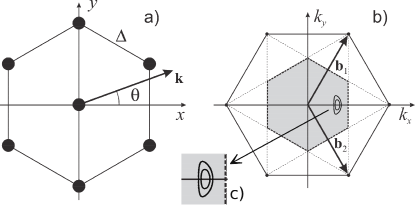
Figure 1: (a) Elementary hexagonal lattice cell with the frame of reference. (b) The reciprocal lattice in ${\bf k}$-space with the basis vectors $|{\bf b}_{1}|=|{\bf b}_{2}|=\frac{4\pi}{\sqrt{3}}\Delta^{-1}$. Due to the lattice symmetry, it is sufficient to consider the wave vectors ${\bf k}$ at $0^{\circ}\leq\theta\leq 30^{\circ}$ and from within the first Brillouin zone (gray region enclosed by dashed lines), so that $|{\bf k}|\Delta\leq\frac{2\pi}{\sqrt{3}}$ for $\theta=0^{\circ}$ and $|{\bf k}|\Delta\leq\frac{4\pi}{3}$ for $\theta=30^{\circ}$. c) Enclosed regions where the particle-wake interactions cause the in-plane and out-of-plane wave modes to merge and form the hybrid mode (see also Fig. 2c). The smaller (larger) region corresponds to the effective dipole moment of wake $\tilde{d}_{\rm eff}=0.7~{}(0.71)$ [Eq. (1)], the screening parameter is $\kappa=1$, the normalized eigenfrequency of the vertical confinement is $\Omega_{\rm conf}=5.66$.

The wakes couple the horizontal and vertical motion of particles in the monolayer. The particle-wake interactions are non-reciprocal Schweigert96 , and therefore under certain conditions the total kinetic energy of the ensemble is no longer conserved: As was shown by Ivlev and Morfill Ivlev01 , when the horizontal and vertical motion are in resonance (which occurs when the out-of-plane and longitudinal in-plane wave modes intersect) the mode-coupling instability sets in. When the gas pressure is low enough and the instability cannot be suppressed by friction, microparticles acquire anomalously high kinetic energy and the crystal melts. The mode-coupling instability and the associated melting has been investigated in numerous theoretical Zhdanov09 ; Roecker12 ; Roecker12eff and experimental works Ivlev03 ; Couedel09 ; Couedel10 ; Couedel11 ; Liu10err ; Liu10corr .

Self-consistent wake models provide better agreement with experimental results Roecker12 ; Roecker12eff . Nevertheless, many theoretical investigations of the mode-coupling instability are still based on a simple “Yukawa/point-wake model” Ivlev01 ; Zhdanov09 , since it makes the analysis of new qualitative effects associated with particle-wake interaction more transparent. In this model, the wake is considered as a positive, point-like effective charge $q$ located at the distance $\delta$ below each particle (of charge $Q$). Thus, the total interaction between two particles is a simple superposition of the particle-particle and particle-wake interactions, both described by the (spherically-symmetric) Yukawa potentials with effective screening length $\lambda$. For a given screening parameter $\kappa=\Delta/\lambda$ the effective dipole moment of wake,

$$\tilde{d}_{\rm eff}=\frac{\tilde{q}\tilde{\delta}}{1-\tilde{q}},$$ (1)

(normalized by $Q\Delta$ and expressed in terms of the dimensionless wake charge $\tilde{q}=q/Q$ and distance $\tilde{\delta}=\delta/\Delta$), determines the growth rate of the mode-coupling instability Couedel11 .

The effective dipole moment is related to parameters of the ambient plasma and can be fairly large for typical experimental conditions Roecker12eff . On the other hand, the theoretical analysis of the mode coupling performed so far was primarily focused on the limit of small $\tilde{d}_{\rm eff}$ Ivlev01 ; Zhdanov09 ; Couedel11 . The question of how the wave modes are modified at large (but still experimentally accessible) values of $\tilde{d}_{\rm eff}$ remains open. Furthermore, while uncoupled in-plane and out-of-plane wave modes (corresponding to purely horizontal and vertical motion, respectively) are linearly polarized, the polarization of waves with a strong wake-induced coupling (when $\tilde{d}_{\rm eff}$ cannot be considered as a small parameter) is a fundamental question which has never been systematically studied.

In this paper we investigate the regime of strong wake-induced coupling between wave modes in 2D plasma crystals. In Sec. II we compare the weak and strong coupling regimes and point out their essential differences. The polarization of separate and hybrid wave modes are discussed in Sec. III. To demonstrate importance of the obtained results for experiments and demonstrate distinct fingerprints of the mixed polarization upon the strong coupling, in Sec. IV we plot representative particle trajectories and spectral densities of the longitudinal and transverse waves, and calculate the shift of the hybridization point.

We normalize the wave number $k$ by the lattice constant $\Delta$, and all frequencies – by the dust-lattice frequency scale,

$$\Omega_{\rm DL}=\sqrt{\frac{(1-\tilde{q})Q^{2}}{M\lambda^{3}}},$$ (2)

viz.,

$$k\Delta\rightarrow k,\qquad\omega/\Omega_{\rm DL},\Omega/\Omega_{\rm DL}\rightarrow\omega,\Omega,$$

where $M$ is the particle mass Ivlev01 ; Zhdanov09 .

II Weak and strong mode coupling

The wake-induced coupling of the in-plane and out-of-plane modes is most efficient for the propagation direction $\theta=0^{\circ}$ Zhdanov09 ; Couedel11 , when ${\bf k}=k{\bf\hat{e}}_{x}$ (see Fig. 1a). In this case, the in-plane transverse (acoustic “shear”) mode becomes exactly decoupled. Therefore, below we assume $\theta=0^{\circ}$ and study the coupling between the remaining two modes Ivlev01 ; Zhdanov09 .

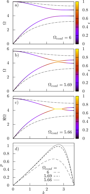
Figure 2: Effect of the wake-induced coupling on the wave modes. (a-c) The colored lines show the (undamped) dispersion relations of the lower and upper modes, $\Omega_{\rm lo,up}(k)$ [Eq. (5)], the dash-dotted lines represent the respective wake-free results, $\Omega_{\rm h,v}(k)$ [Eq. (21) with $\tilde{q}=0$]. The curves are obtained for three different values of the vertical confinement frequency $\Omega_{\rm conf}$. In (a) the modes are attracted to each other, in (b) the gap between the modes is getting constricted, and in (c) they merge and form the hybrid mode (only the real part is shown). The color-coding shows the circularity of the mode polarization, $\epsilon$, which is determined by the reduced coupling parameter [Eqs (10) and (14) for the separate and hybrid modes, respectively]. (d) The coupling parameter $p(k)$ [Eq. (6)] for panels (a-c), the modes merge at $p=1$. The results are for $\kappa=1$, the dimensionless wake charge $\tilde{q}=0.7$, the wake length $\tilde{\delta}=0.3$ ($\tilde{d}_{\rm eff}=0.7$).

The exact dispersion relations $\omega(k)$ of the coupled in-plane and out-of-plane wave modes for $\theta=0^{\circ}$ are determined by the following equation Ivlev01 ; Zhdanov09 ; Couedel11 :

$$\left[\omega(\omega+i\nu)-\Omega^{2}_{\rm h}\right]\left[\omega(\omega+i\nu)-\Omega^{2}_{\rm v}\right]+\sigma^{2}=0,$$ (3)

where $\Omega_{\rm h,v}(k)$ are the eigenfrequencies of the horizontal (in-plane) and vertical (out-of-plane) modes in the absence of coupling, $\sigma(k)>0$ is the coupling term, and $\nu$ is the damping rate due to neutral gas friction Epstein24 . Expressions for $\Omega^{2}_{\rm h,v}$ and $\sigma$ are given in Appendix A (wake-free results are obtained by putting the wake charge $\tilde{q}$ equal to zero). Adopting the notation $\Omega^{2}=\omega(\omega+i\nu)$, Eq. (3) can be written in a form of the eigenvalue problem Zhdanov09 ; Couedel11 ,

$$\det(\textsf{D}_{k}-\Omega^{2}\textsf{I})=0,\qquad\textsf{D}_{k}=\left(\begin{array}[]{cc}\Omega^{2}_{\rm h}&i\sigma\\ i\sigma&\Omega^{2}_{\rm v}\end{array}\right),$$ (4)

where I denotes the unit matrix and $\textsf{D}_{k}$ is the non-Hermitian dynamical matrix (note that $\textsf{D}_{k}^{*}=\textsf{D}_{-k}$). The squared eigenfrequencies of the lower and upper modes,

$$\Omega_{\rm lo,up}^{2}=\frac{\Omega^{2}_{\rm v}+\Omega^{2}_{\rm h}}{2}\mp\frac{\Omega^{2}_{\rm v}-\Omega^{2}_{\rm h}}{2}\sqrt{1-p^{2}},$$ (5)

are determined by the reduced coupling parameter $p(k)$,

$$p=\frac{2\sigma}{\Omega^{2}_{\rm v}-\Omega^{2}_{\rm h}}.$$ (6)

When $p\rightarrow 0$ the lower and upper modes are reduced to the horizontal and vertical modes, respectively, i.e., $\Omega_{\rm lo,up}(k)\rightarrow\Omega_{\rm h,v}(k)$.

The eigenfrequencies of the upper and lower modes are real and different for $p<1$ – in this regime we shall call the modes separate. For $p>1$ the eigenfrequencies become complex conjugate (i.e., with equal real parts), and therefore the resulting lower and upper modes are referred to as hybrid; in this case, $\Omega_{\rm lo,up}$ in Eq. (5) has to be replaced with $\Omega^{{\rm(hyb)}}_{\rm lo,up}$. The eigenfrequencies of the lower and upper hybrid modes have negative and positive imaginary parts, respectively, so that the former is decaying and the latter is growing. The hybrid modes emerge at the critical point $p=1$, which occurs at the critical wave number $k=k_{\rm cr}$ when the critical confinement $\Omega_{\rm conf}=\Omega_{\rm cr}$ is reached.

Thus, the wake-induced mode coupling can be considered as a non-equilibrium second-order phase transition, where $p$ plays the role of the control parameter, while the imaginary part of the hybrid eigenfrequency, $\Im\Omega^{\rm(hyb)}$, is the proper order parameter.

The lower and upper modes near the onset of hybridization are illustrated in Fig. 2a-c for three characteristic values of the vertical confinement frequency, $\Omega_{\rm conf}$ (for simplicity we consider undamped waves). The corresponding coupling parameters $p(k,\Omega_{\rm conf})$ are plotted in Fig. 2d, so that $\Omega_{\rm conf}$ plays the role of the control parameter. In Fig. 2a the branches $\Omega_{\rm lo}(k)$ and $\Omega_{\rm up}(k)$ are noticeably attracted to each other near $k\simeq 2.7$, where the maximum of $p(k)$ is reached; although $p_{\rm max}\simeq 0.67$ is still well below unity, the deviation from the wake-free results $\Omega_{\rm h,v}(k)$ is already quite significant. In Fig. 2b, where $p_{\rm max}\simeq 0.97$, one can see that the gap between the modes becomes constricted. In Fig. 2c, where $\Omega_{\rm conf}>\Omega_{\rm cr}$, the modes merge and form the hybrid branch in the range of $k$ where $p(k)\geq 1$ [$\Re\Omega^{\rm(hyb)}(k)$ is shown]. In the ${\bf k}$-plane, the hybrid modes are located in an enclosed region, as illustrated in Figs 1b,c.

The magnitude of the coupling term $\sigma$ is determined by the effective dipole moment of the wake [see, e.g., Eq. (21)]. For the example presented in Fig. 2 we choose $\tilde{d}_{\rm eff}=0.7$, which is rather large but quite realistic for experiments (see, e.g. Ivlev03 ; Couedel10 ; Liu10corr ). As we can see, in this case the critical point and hence the hybrid branch are significantly shifted away from the border of the Brioullin zone, where the hybrid mode is localized in the limit of weak coupling [since the uncoupled branches $\Omega_{\rm h,v}(k)$ are monotonic].

The “attraction effect” between the modes seen in Fig. 2a-c has not been carefully studied before, since theoretical analysis of the mode coupling performed so far was primarily focused on the limit of small $\sigma$ Ivlev01 ; Zhdanov09 ; Couedel11 . As we can see from Eq. (6), the critical point in this limit is reached when the uncoupled branches practically cross. From Fig. 2 it is evident that for finite $\sigma$ the merging occurs well before the crossing (which now corresponds to $p\rightarrow\infty$).

In what follows we shall always consider a weak neutral damping, viz., $\nu\ll\Omega_{\rm lo,up}$, which is the typical situation for experiments Couedel09 ; Couedel10 ; Ivlev03 . In this case the dispersion relations $\omega_{\rm lo,up}(k)$ are obtained by simply adding $-\frac{1}{2}\nu$ to the imaginary part of $\Omega_{\rm lo,up}(k)$, i.e.,

$$\omega_{\rm lo,up}(k)\simeq\Omega_{\rm lo,up}(k)-i\frac{\nu}{2}.$$ (7)

On the other hand, we shall assume the damping to be sufficiently strong to suppress the mode-coupling instability, viz., $\nu>2|\Im\Omega^{\rm(hyb)}(k)|$. This ensures that the kinetic temperature of particles can reach a steady-state level which is low enough to keep the crystalline order, i.e., the hybrid mode can still be observed in experiments.

III Polarization of wave modes

From the eigenvectors $\boldsymbol{\zeta}_{\alpha}$ of the dynamical matrix (where $\alpha=$ lo, up) we obtain the wave modes ${\bf w}_{\alpha}$. The separate modes are

$${\bf w}_{\alpha}=\boldsymbol{\zeta}_{\alpha}e^{ikx-i\omega_{\alpha}(k)t}+c.c.,$$ (8)

where $c.c.$ denotes the complex conjugate, and the hybrid modes ${\bf w}_{\alpha}^{\rm(hyb)}$ are similarly obtained from $\boldsymbol{\zeta}^{\rm(hyb)}_{\alpha}$.

Polarization of the modes can be conveniently characterized by the “real phases”,

$$\Phi_{\alpha}\equiv kx-\Re\Omega_{\alpha}t,$$

and the “circularity” $\epsilon$: $0$ and $1$ stand for the linear and circular polarizations, respectively, $0<\epsilon<1$ are for elliptical polarization. For the separated and hybridized regimes the circularity is given by certain functions of the reduced coupling parameter $p$ (see below).

III.1 Separate modes ($p<1$)

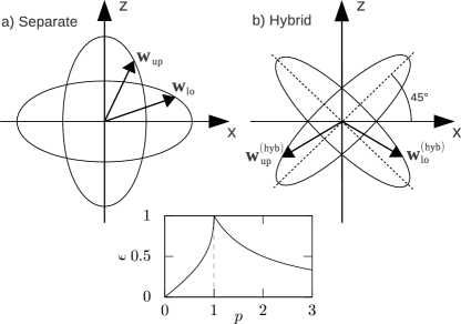
Figure 3: Lissajous ellipses of the lower/upper separate modes ${\bf w}_{\rm lo,up}$ [Eq. (11)] and lower/upper hybrid modes ${\bf w}^{\rm(hyb)}_{\rm lo,up}$ [Eq. (13)]. For the separate modes the major axes of the ellipses are along the coordinate axes, for the hybrid modes the axes remain mutually orthogonal, but are rotated by $45^{\circ}$. The shape of the ellipses is determined by the circularity $\epsilon$: For $\epsilon=0$ the ellipses degenerate into lines, for $\epsilon=1$ they form a circle (the illustration is for $\epsilon=0.5$). The inset below shows the dependence of $\epsilon$ on the reduced coupling parameter $p$, which is determined by Eqs (10) and (14) for the separate and hybrid modes, respectively.

Uncoupled ($p\rightarrow 0$) horizontal and vertical wave modes are linearly polarized ($\epsilon\rightarrow 0$) and the corresponding dynamical matrix is purely real (Hermitian) Zhdanov09 . Hence, the uncoupled eigenvectors are mutually orthogonal and real. For finite $p$ we obtain

$$\boldsymbol{\zeta}_{\rm lo}=\frac{\left(1,\;-i\epsilon\right)}{\sqrt{1+\epsilon^{2}}},\quad\boldsymbol{\zeta}_{\rm up}=\frac{\left(i\epsilon,\;1\right)}{\sqrt{1+\epsilon^{2}}},$$ (9)

so that $|{\boldsymbol{\zeta}}_{\alpha}|^{2}=1$ and the circularity $\epsilon$ is the following function of $p$:

$$\epsilon=p/(1+\sqrt{1-p^{2}}).$$ (10)

Thus, the lower and upper modes expressed via the corresponding wave phases,

$$\begin{array}[]{r}{\displaystyle{\bf w}_{\rm lo}=\frac{2e^{-\frac{1}{2}\nu t}}{{\sqrt{1+\epsilon^{2}}}}\left(\cos\Phi_{\rm lo},\;\epsilon\sin\Phi_{\rm lo}\right),\vspace{0.2cm}}\\ {\displaystyle{\bf w}_{\rm up}=\frac{2e^{-\frac{1}{2}\nu t}}{{\sqrt{1+\epsilon^{2}}}}\left(-\epsilon\sin\Phi_{\rm up},\;\cos\Phi_{\rm up}\right),}\end{array}$$ (11)

are parametric functions of the two ellipses illustrated in Fig. 3a.

Figure 2 shows that for $k\ll 1$ as well as for $k$ near the border of the first Brillouin zone the coupling parameter $p$ is very small and therefore both ${\bf w}_{\rm lo}$ and ${\bf w}_{\rm up}$ are linearly polarized ($\epsilon\rightarrow 0$). For $k$ where $p\simeq p_{\rm max}$ the circularity becomes significant and the polarization is essentially elliptical. At the points where the upper and lower separate branches merge and form the hybrid branch (Fig. 2c) the modes are circularly polarized ($\epsilon=1$).

III.2 Hybrid modes ($p\geq 1$)

For $p=1$ the modes are degenerate. Hence, the eigenvectors for the separate modes [Eq. (9)] and hybrid modes should coincide at this point, which yields

$$\begin{array}[]{r}{\displaystyle{\boldsymbol{\zeta}}^{\rm(hyb)}_{\rm lo}=\frac{1}{\sqrt{2}}\left(1,\;-i\epsilon-\sqrt{1-\epsilon^{2}}\right),\vspace{0.2cm}}\\ {\displaystyle{\boldsymbol{\zeta}}^{\rm(hyb)}_{\rm up}=\frac{1}{\sqrt{2}}\left(i\epsilon+\sqrt{1-\epsilon^{2}},\;1\right).}\end{array}$$ (12)

The lower and upper hybrid modes,

$$\begin{array}[]{r}{\displaystyle{\bf w}^{\rm(hyb)}_{\rm lo}=\sqrt{2}e^{-\frac{1}{2}(\gamma+\nu)t}\;\{\cos\Phi_{\rm lo},\;\sin(\Phi_{\rm lo}-\Phi_{0})\},\vspace{0.2cm}}\\ {\displaystyle{\bf w}^{\rm(hyb)}_{\rm up}=\sqrt{2}e^{\frac{1}{2}(\gamma-\nu)t}\;\{-\sin(\Phi_{\rm up}-\Phi_{0}),\;\cos\Phi_{\rm up}\},}\end{array}$$ (13)

are parametric functions of the two ellipses shown in Fig. 3b. Here, $\gamma(k)\equiv 2|\Im\Omega^{\rm(hyb)}(k)|$ is the damping (growth) rate of the lower (upper) hybrid mode, the circularity $\epsilon$ and phase shift $\Phi_{0}$ are given by

$$\epsilon=\cos\Phi_{0}=p^{-1}.$$ (14)

We see that the major polarization axes of the hybrid modes (remaining mutually orthogonal) are rotated by $45^{\circ}$ with respect to the axes of separate modes. The rotation occurs discontinuously at $p=1$ (where the degenerate modes are circularly polarized). Unlike the separate modes, the hybrid mode circularity decreases with $p$ (see inset in Fig. 3), i.e., the hybrid modes are always elliptically polarized between the merging points (see Fig. 2c). Furthermore, upon the crossing of the horizontal and vertical branches, $\Omega_{\rm v}^{2}-\Omega_{\rm h}^{2}\to 0$, the coupling $p$ diverges at the crossing point and the polarization of hybrid modes becomes linear near the intersection.

So far, reliable experimental results on the onset of the mode-coupling instability have been only obtained for a slightly over-critical coupling. The reason for that is rather simple – upon a “deep quenching” the crystal cannot be observed long enough (to deduce sufficiently accurate dispersion relations) before it is completely destroyed by the instability. Such conditions (e.g., of Fig. 2c) yield slightly distorted circular polarization ($0.95\lesssim\epsilon\leq 1$) along the whole hybrid branch.

IV Features of strong coupling: Examples

The strong mode coupling introduces several characteristic features which are expected to be revealed upon analysis of corresponding experiments. Below we discuss some of the most interesting phenomena characterizing the individual particle motion as well as the wave modes near the hybridization point.

IV.1 Particle trajectories

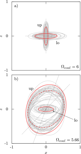
Figure 4: Characteristic particle trajectories representing the lower and upper wave modes for the time interval of $50~{}\Omega_{\rm DL}^{-1}$. All parameters of (a) and (b) correspond to Fig. 2a and c, respectively, $x$ and $z$ are in arbitrary units. The solid-line ellipses depict “orbitals” (straight dotted lines indicate their major axes) inside which the particles mostly reside. In the separated regime (a), the major axes are along the coordinate axes. In the hybridized regime (b), the major axis for the (decaying) lower mode is practically horizontal, while for (growing) upper mode it is rotated by $\simeq 70^{\circ}$. The dashed-line ellipse shows the contribution from the upper hybrid branch only.

The individual particle trajectories are calculated by applying the inverse Fourier transform (over $k$) to the wave modes, Eqs (11) and (13). Thus, each trajectory can be viewed as the weighted “superposition” of the Lissajous ellipses (at a given $k$), with the weights determined by the magnitudes of the corresponding eigenvectors. The gray lines in Fig. 4 illustrate the resulting steady-state trajectories (when friction is on average balanced by the thermal noise, see Sec. IV.2 for details) for the separated (a) and hybridized (b) regimes. The trajectories are shown for the time interval of $50~{}\Omega_{\rm DL}^{-1}$, which corresponds to $\sim 3$ s under typical experimental conditions Couedel11 . We also draw “orbitals” (solid-line ellipses), to indicate the areas mostly covered by the trajectories (i.e., where particles reside most of the time). Due to stronger vertical confinement in the separated regime (Fig. 4a), the vertical extent of the upper-mode orbital is somewhat smaller than the horizontal size of the lower-mode orbital.

In the hybridized regime illustrated in Fig. 4b, the trajectories are determined by the superposition of (weighted) contributions from the separate and hybrid branches (see Fig. 2c). As one can conclude from Fig. 3, this yields a “superposition” of ellipses oriented along the coordinate axes and those rotated by $45^{\circ}$. The hybrid branches are formed within a relatively small region of the Brillouin zone, yet the amplitude of the upper branch can be significantly increased, while for the lower branch it is reduced [see Eq. (13)]. All this governs the size and orientation of the corresponding orbitals: The lower orbital is practically horizontal and its size is similar to that in Fig. 4a, since the amplitude for the lower hybrid branch is too small and hence the separate branch provides the major contribution here. Contrary, the upper orbital is large and rotated by an angle notably smaller than $90^{\circ}$ (but larger than $45^{\circ}$), since the major contribution in this case is from the enhanced hybrid branch (the corresponding orbital is indicated by the dashed-line ellipse).

IV.2 Mode spectral density

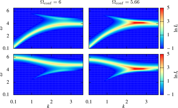
Figure 5: Longitudinal (upper panel) and transverse (lower panel) mode spectral densities $I_{\rm l,t}(k,\omega)$. Figures on the left show the results calculated from Eq. (17) for the separate modes, on the right the results from Eq. (18) for the hybrid modes are presented (all parameters correspond to Figs 2a and 2c, respectively). In the separated regime, the lower mode (longitudinal without coupling) has a transverse component, the upper mode (transverse without coupling) has a longitudinal component. The longitudinal and transverse densities of the hybrid modes are equal, which follows from the orientation of their polarization ellipses (see Fig. 3b). The shown example is for the normalized damping rate $\nu=0.3$, the spectral density is in units of $I_{0}$.

Experimentally, fluctuation wave spectra (dispersion relations) are extracted from the observation of the particle motion which is triggered by thermal noise and damped by neutral gas friction Nunomura02 ; Couedel09 ; Couedel10 .

The scenario can be mimicked by the Langevin equation, where the stochastic excitation force on each particle is uncorrelated and described by the Gaussian white noise Schwabl ; Zhdanov03 ; VanKampenBook . We write the force in the form $M{\bf a}(t)$, where the elements $a_{j}$ of the stochastic acceleration are defined by the first two stochastic moments, $\langle a_{j}(t)\rangle=0$ and $\langle a_{j}(t)a_{k}(t^{\prime})\rangle=(2\nu T/M)\delta_{jk}\delta(t-t^{\prime})$ (as it follows from the fluctuation-dissipation theorem). Here, $\delta_{jk}$ is the Kronecker delta function ($j,k=x,y,z$) and $T$ is the relevant kinetic temperature (determined by the temperature of neutral gas and mechanisms of individual dust “heating” operating in a plasma, e.g., due to charge variations Vaulina99 ; Ivlev00 ; Nunomura99 ; Pustylnik06 ).

The perturbations for the separate modes read

$$\tilde{\boldsymbol{\zeta}}=\sum_{\alpha=\rm lo,up}\frac{\left({\bf a}^{(k\omega)}\cdot\boldsymbol{\zeta}_{\alpha}\right)\boldsymbol{\zeta}_{\alpha}}{[\Omega_{\alpha}^{2}(k)-\omega(\omega+i\nu)]\zeta_{\alpha}^{2}},$$ (15)

where $\zeta_{\alpha}^{2}\equiv\boldsymbol{\zeta}_{\alpha}\cdot\boldsymbol{\zeta}_{\alpha}$ and ${\bf a}^{(k\omega)}$ is the Fourier transform of the stochastic acceleration over all particles; for the hybrid modes, the superscript “(hyb)” has to be added.

For a monolayer comprised of $N$ particles, the total kinetic energy is

$$K=\frac{1}{2}M\sum_{j=1}^{N}\left\langle v_{j}^{2}\right\rangle\equiv N\int d{\bf k}\int d\omega\;I({\bf k},\omega).$$ (16)

Here $I({\bf k},\omega)=I_{\rm l}({\bf k},\omega)+I_{\rm t}({\bf k},\omega)$ is the spectral density of thermal fluctuations, which consists of the longitudinal and transverse components (with respect to ${\bf k}=k{\bf\hat{e}}_{x}$, the ${\bf k}$-integration is over the first Brillouin zone). By representing $K$ via the Fourier-transformed particle velocities with the components $v^{(k\omega)}_{\rm l,t}=-i\omega\tilde{\zeta}_{x,z}$, we obtain the spectral density components expressed in terms of the horizontal and vertical eigenfrequencies:

$$I_{\rm l,t}(k,\omega)=I_{0}\omega^{2}\frac{\sigma^{2}+|A_{\rm v,h}|^{2}}{|\sigma^{2}+A_{\rm v}A_{\rm h}|^{2}}$$ (17)

where $A_{\rm h,v}(k,\omega)\equiv\Omega_{\rm h,v}^{2}(k)-\omega(\omega+i\nu)$. The spectral density scale $I_{0}=\sqrt{3}\Delta^{2}\nu T/\left(16\pi^{3}\Omega^{2}_{\rm DL}\right)$ has the dimensionality of J$\cdot$cm${}^{2}\cdot$s (here $\nu$ is not normalized!).

Remarkably, $I_{\rm l}(k,\omega)$ of the separate modes shows not only a bright longitudinal, but also a weak transverse component, and vice versa for $I_{\rm t}(k,\omega)$ (see left panel of Fig. 5). When the coupling is intermediate-to-strong ($0.3\lesssim p\lesssim 0.95$, see Fig. 2d) the “weak” components become fairly bright. For a small coupling ($p\ll 1$) Eq. (17) is reduced to $I_{\rm l,t}(k,\omega)\simeq I_{0}\omega^{2}\big{|}{\Omega^{2}_{\rm h,v}(k)-\omega(\omega+i\nu)}\big{|}^{-2}$ and the weak components disappear. Qualitative interpretation of these results is straightforward: The mode polarization changes between linear and elliptical, and therefore we find the “weak” components varying between zero and their peak brightness. The latter is smaller than the density of the “strong” components, since the modes are still separated.

From the orientation of polarization ellipses of the hybrid modes (Fig. 3, $p>1$), it is evident that their longitudinal and transverse spectral densities are equal along the hybrid branch (see right panel of Fig. 5). These densities are

$$I_{\rm l}^{\rm(hyb)}(k)=I_{\rm t}^{\rm(hyb)}(k)$$

$$=I_{0}\frac{\nu^{2}+(p^{2}+1)B}{[\nu^{2}-(p^{2}-1)B]^{2}},$$ (18)

where $B(k)=\frac{1}{2}(\Omega_{\rm v}^{2}-\Omega_{\rm h}^{2})^{2}(\Omega_{\rm v}^{2}+\Omega_{\rm h}^{2})^{-1}$. In accordance with Eq. (13), the decay rate of the lower hybrid mode is added to the neutral damping rate $\nu$, while the growth rate of the upper mode is subtracted. Therefore, the relative contribution of the lower hybrid mode to the total spectral density in Eq. (18) is relatively small. The density naturally diverges if the damping threshold of the mode-coupling instability is reached [at the maximum of $p(k)$].

Figure 5 indicates that the spectral density distribution along the hybrid branch can be slightly asymmetric (with respect to the center). This is because the functions $p(k)$ and $B(k)$ are slightly asymmetric as well (see Fig. 2c,d). This feature might be important for the analysis of high-resolution experimental spectra Couedel09 ; Couedel10 ; Couedel11 ; Liu10err ; Liu10corr .

IV.3 Shift of the critical point

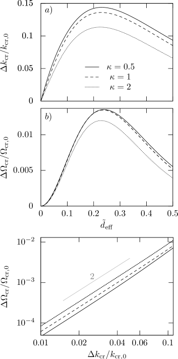
Figure 6: The relative shift (a) of the critical wave number, $\Delta k_{\rm cr}/k_{\rm cr,0}$, and (b) of the critical confinement, $\Delta\Omega_{\rm cr}/\Omega_{\rm cr,0}$, as a function of the effective dipole moment of wake $\tilde{d}_{\rm eff}$. (c) Relation between the shifts, showing that it is very close to $\Delta\Omega_{\rm cr}\propto(\Delta k_{\rm cr})^{2}$. The results are for $\tilde{q}=0.4$ and three different values of $\kappa$.

In the limit of weak mode coupling, the hybridization sets in upon the crossing of the uncoupled branches $\Omega_{\rm h}(k)$ and $\Omega_{\rm v}(k)$. The critical point in this case is located at the border of the first Brillouin zone, $k_{\rm cr,0}=\frac{2\pi}{\sqrt{3}}$ (see Fig. 1b), and the corresponding critical confinement is $\Omega_{\rm cr,0}$. As one can see from Fig. 2a-c, in the regime of strong coupling the critical point is shifted towards smaller $k$ and occurs at higher confinement. Hence, we can write

$$k_{\rm cr}=k_{\rm cr,0}-\Delta k_{\rm cr},\qquad\Omega_{\rm cr}=\Omega_{\rm cr,0}+\Delta\Omega_{\rm cr}.$$ (19)

In Appendix B we derive universal expressions for $k_{\rm cr}$ and $\Omega_{\rm cr}/\Omega_{\rm cr,0}$ which are functions of the wake parameters $\tilde{q}$ and $\tilde{\delta}$ (for a given $\kappa$). Let us analyze the obtained results.

The functional dependence of $\Delta k_{\rm cr}$ on the wake parameters is governed by the competition of two effects: (i) Increase of the effective dipole moment $\tilde{d}_{\rm eff}$ makes the “mode attraction” stronger, which causes $\Delta k_{\rm cr}$ to increase. (ii) Increase of the wake length $\tilde{\delta}$ weakens the screened wake-particle interaction, which forces $\Delta k_{\rm cr}$ to decrease. Figure 6a illustrates these effects. We fixed the wake charge $\tilde{q}$ and vary the wake length $\tilde{\delta}$ (and, hence, the dipole moment): When $\tilde{\delta}$ is sufficiently small ($\lesssim 0.2$), the effect (i) obviously dominates, resulting in an almost linear increase of $\Delta k_{\rm cr}$ with the dipole moment; the maximum is reached at $\tilde{d}_{\rm eff}\simeq 0.22$. For larger $\tilde{\delta}$ ($\gtrsim 0.3$), the effect (ii) becomes more important and $\Delta k_{\rm cr}$ starts to decrease. When the wake length is so large that the particle-wake interactions are strongly screened ($\kappa\tilde{\delta}\gtrsim 2-3$), $\Delta k_{\rm cr}$ rapidly falls off and the modes become weakly coupled again.

It is noteworthy that the $k$-shift of the critical point can be really significant (up to $\simeq 15\%$), making the effect experimentally observable.

The dependence of $\Delta\Omega_{\rm cr}$ on $\tilde{d}_{\rm eff}$ shown in Fig. 6b follows essentially the same trend, since the two effects mentioned above equally work for the shift of the critical confinement. However, the magnitude of $\Delta\Omega_{\rm cr}$ turns out to be much smaller than that of $\Delta k_{\rm cr}$ (${\Delta\Omega_{\rm cr}}/{\Omega_{\rm cr,0}}\lesssim 2\%$) and therefore is practically negligible. To a very good accuracy, $\Delta\Omega_{\rm cr}/{\Omega_{\rm cr,0}}$ is a parabolic function of $\Delta k_{\rm cr}$, as shown in Fig. 6c.

Note that these results can be also obtained from a simple 1D string model with next-neighbor interactions Ivlev01 . The 1D model provides compact analytical expressions for $\Delta k_{\rm cr}$ and ${\Delta\Omega_{\rm cr}}/{\Omega_{\rm cr,0}}$ [see Eqs (22) and (23)] which are convenient for order-of-magnitude estimates. The main qualitative difference from the rigorous calculations is that the approximate results become independent of $\kappa$ in the limit of small $\tilde{d}_{\rm eff}$ (compare with Fig. 6).

V Summary and Conclusion

In this paper we discussed effects of strong wake-induced coupling between dust-lattice wave modes in 2D plasma crystals. So far, the mode coupling occurring due to nonreciprocal particle-wake interactions (and resulting in the mode-coupling instability, the major plasma-specific mechanism of melting of 2D crystals) has been systematically studied only in the weak regime, when the effective dipole moment of wake is assumed to be sufficiently small Zhdanov09 ; Couedel10 ; Roecker12 ; Roecker12eff . In this case, the longitudinal in-plane and out-of-plane modes (participating in the coupling) were shown to be strongly modified only in a small vicinity of their crossing, where they form the hybrid mode.

In fact, the regime of strong mode coupling has been already achieved in several experiments Ivlev03 ; Couedel10 ; Liu10corr , and therefore careful analysis of its implications is absolutely necessary for further studies of 2D plasma crystals. Below we summarize the most notable features of the strong mode coupling:

1. The two coupled wave modes corresponding to the in-plane and out-of-plane motion are significantly modified in a broad range of wave numbers – the branches become “attracted” to each other even before they merge and form the hybrid modes. The modified modes are called, respectively, “lower” and “upper”, to distinguish from the weak-coupling regime.

2. Unlike the weak-coupling regime, the polarization of the two modes becomes essentially elliptical before the hybridization: The (originally longitudinal) lower mode can have a significant transverse component, the (originally transverse) upper mode has a longitudinal component.

3. The polarization of the hybrid modes is circular at the merging ends, and is (weakly) elliptical in the middle of the hybrid branch. The polarization ellipses in this case are rotated by $45^{\circ}$ with respect to the polarization of the separate modes, and therefore the hybrid mode spectral density has equal longitudinal and transverse components.

4. The individual particle trajectories for the separate modes are localized within ellipsoidal “orbitals” with the mutually orthogonal axes. Upon the hybridization, the orbital representing the (growing) upper mode is significantly increased and rotated by an angle notably larger than $45^{\circ}$.

5. The location of the hybrid mode can be significantly shifted towards smaller wave numbers, away from the border of the Brioullin zone (where the hybrid mode is formed for a weak coupling). The relative magnitude of the effect can be as high as $\simeq 15\%$.

It would be highly desirable to perform accurate experimental measurements of the individual particle trajectories and wave fluctuation spectra (performed with increased signal-to-noise ratio). The analysis of such trajectories and spectra would make it possible to reveal (at least) some of the above-mentioned features. The theory presented in this paper provides direct relation between the magnitude of the strong-mode-coupling effects (such as the wave polarization, distribution of the fluctuation intensity, shift of the hybrid mode) and the principal characteristics of the plasma wakes.

Appendix A Elements of the dynamical matrix $\textsf{D}_{k}$

We introduce utility functions

$$h_{1}(\kappa)=e^{-\kappa}(\kappa^{-1}+2\kappa^{-2}+2\kappa^{-3}),$$

$$h_{2}(\kappa)=e^{-\kappa}(\kappa^{-2}+\kappa^{-3}),$$

$$h_{3}(\kappa)=h_{1}(\kappa)+h_{2}(\kappa),$$

to be used for expressions of the elements of $\textsf{D}_{k}$ [Eq. (4)]. For the 1D string model with next-neighbor interactions Ivlev01 we have:

$$\Omega^{2}_{\rm h}=\frac{4}{1-\tilde{q}}\left(h_{1}(\kappa)+\tilde{q}h_{2}(\tilde{\kappa})-\frac{\tilde{q}}{1+\tilde{\delta}^{2}}h_{3}(\tilde{\kappa})\right)\sin^{2}\frac{1}{2}k,$$

$$\Omega^{2}_{\rm v}=\Omega^{2}_{\rm conf}-\frac{4}{1-\tilde{q}}\left(h_{2}(\kappa)-\tilde{q}h_{2}(\tilde{\kappa})+\frac{\tilde{q}\tilde{\delta}^{2}}{1+\tilde{\delta}^{2}}h_{3}(\tilde{\kappa})\right)\sin^{2}\frac{1}{2}k,$$ (20)

$$\sigma=2\frac{\tilde{q}\tilde{\delta}}{(1-\tilde{q})(1+\tilde{\delta}^{2})}h_{3}(\tilde{\kappa})\sin k.$$

where $\tilde{\kappa}=\kappa\sqrt{1+\tilde{\delta}^{2}}$.

The rigorous results for 2D monolayers are obtained by taking into account interactions with all neighbors Zhdanov09 ; Couedel11 . For the wave vector ${\bf k}=k{\bf\hat{e}}_{x}$, the elements of $\textsf{D}_{k}$ are:

$$\Omega^{2}_{\rm h}=\frac{2}{1-\tilde{q}}\sum_{m,n}\left(\frac{s^{2}_{x}}{s^{2}}h_{1}(\kappa s)-\frac{s^{2}_{y}}{s^{2}}h_{2}(\kappa s)+\tilde{q}h_{2}(\kappa s_{\delta})-\tilde{q}\frac{s^{2}_{x}}{s^{2}_{\delta}}h_{3}(\kappa s_{\delta})\right)\sin^{2}\frac{1}{2}ks_{x},$$

$$\Omega^{2}_{\rm v}=\Omega^{2}_{\rm conf}-\frac{2}{1-\tilde{q}}\sum_{m,n}\left(h_{2}(\kappa s)-\tilde{q}h_{2}(\kappa s_{\delta})+\tilde{q}\frac{\tilde{\delta}^{2}}{s^{2}_{\delta}}h_{3}(\kappa s_{\delta})\right)\sin^{2}\frac{1}{2}ks_{x},$$ (21)

$$\sigma=\frac{\tilde{q}\tilde{\delta}}{1-\tilde{q}}\sum_{m,n}\frac{s_{x}}{s^{2}_{\delta}}h_{3}(\kappa s_{\delta})\sin ks_{x},$$

where $s_{x}=\sqrt{3}m/2$, $s_{y}=m/2+n$, $s=\sqrt{m^{2}+n^{2}+mn}$, $s_{\delta}=\sqrt{s^{2}+\tilde{\delta}^{2}}$, the summation is over all integers except $(0,0)$.

Appendix B Shift of the critical point [Eq. (19)]

The critical wave number $k_{\rm cr}$ and critical confinement frequency $\Omega_{\rm cr}$ for the onset of hybridization are determined from the following conditions on the reduced coupling parameter: $p(k_{\rm cr},\Omega_{\rm cr})=1$ and $\partial p/\partial k|_{k_{\rm cr},\Omega_{\rm cr}}=0$.

For the 1D string model we use Eq. (20), which yields:

$$\Delta k_{\rm cr}=\arctan{\mathcal{D}},\quad\frac{\Omega^{2}_{\rm cr}}{\Omega^{2}_{\rm cr,0}}=\frac{1}{2}\left(1+\sqrt{1+{\mathcal{D}}^{2}}\right),$$ (22)

where

$${\mathcal{D}}=\frac{2\tilde{q}\tilde{\delta}h_{3}(\tilde{\kappa})}{(1+\tilde{\delta}^{2})h_{3}(\kappa)-\tilde{q}(1-\tilde{\delta}^{2})h_{3}(\tilde{\kappa})}.$$

For small $\tilde{\delta}$ we get ${\mathcal{D}}\to 2\tilde{q}\tilde{\delta}/(1-\tilde{q})\equiv 2\tilde{d}_{\rm eff}$. Thus, in the weak-coupling regime we get a simple universal relation between $\Delta k_{\rm cr}$ and $\Delta\Omega_{\rm cr}$,

$$\frac{\Delta\Omega_{\rm cr}}{\Omega_{\rm cr,0}}\simeq\frac{1}{8}\left(\Delta k_{\rm cr}\right)^{2}\simeq\frac{1}{2}\tilde{d}_{\rm eff}^{2}.$$ (23)

For the rigorous 2D model we employ Eq. (21) and obtain the following equations for $k_{\rm cr}$ and $\Omega_{\rm cr}$:

$$\begin{array}[]{r}{\displaystyle\sum_{m,n}s_{x}\big{(}{\mathcal{A}}\cos k_{\rm cr}s_{x}+{\mathcal{B}}\sin k_{\rm cr}s_{x}\big{)}=0,\vspace{0.2cm}}\\ {\displaystyle\frac{\Omega^{2}_{\rm cr}}{\Omega^{2}_{\rm cr,0}}=\frac{\sum_{m,n}\left[{\mathcal{A}}\sin k_{\rm cr}s_{x}+{\mathcal{B}}\left(1-\cos k_{\rm cr}s_{x}\right)\right]}{\sum_{m,n}{\mathcal{B}}\left[1-(-1)^{m}\right]},}\end{array}$$ (24)

where

$${\mathcal{A}}(\tilde{q},\tilde{\delta},\kappa)=4\tilde{q}\tilde{\delta}\frac{s_{x}}{s^{2}_{\delta}}h_{3}(\kappa s_{\delta}),$$

$${\mathcal{B}}(\tilde{q},\tilde{\delta},\kappa)=2\frac{s^{2}_{x}}{s^{2}}h_{3}(\kappa s)-2\tilde{q}\frac{s_{x}^{2}-\tilde{\delta}^{2}}{s^{2}_{\delta}}h_{3}(\kappa s_{\delta}).$$

The first equation (24) yields $k_{\rm cr}$, which should then be substituted to the second equation to obtain $\Omega_{\rm cr}$.

References

- (1) P.K. Shukla and A.A. Mamun, Introduction to Dusty Plasma Physics (IoP Publishing, 2002).
- (2) V. E. Fortov, A. V. Ivlev, S. A. Khrapak, A. G. Khrapak, and G. E. Morfill, Phys. Rep. 421, 1 (2005).
- (3) P.K. Shukla and B. Eliasson, Rev. Mod. Phys. 81, 25 (2003).
- (4) M. Bonitz, C. Henning and D.Block, Rep. Progr. Phys. 73, 6 (2010).
- (5) V. Fortov and G. Morfill, Complex and Dusty Plasmas (CRC Press, 2010).
- (6) G. E. Morfill and A. V. Ivlev, Rev. Mod. Phys. 81, 1353 (2009).
- (7) A. Ivlev, H. Löwen, G. Morfill, C. P. Royall, Complex Plasmas and Colloidal Dispersions (World Scientific, 2012).
- (8) J. H. Chu and L. I, Phys. Rev. Lett. 72, 4009 (1994).
- (9) H. Thomas, G.E. Morfill, V. Demmel, J. Goree, B. Feuerbacher and D. Möhlmann, Phys. Rev. Lett. 73, 652 (1994).
- (10) F. Melandsö and J. Goree, Phys. Rev. E 52, 5312 (1995).
- (11) S. V. Vladimirov and A. A. Samarian, Phys. Rev. E 65, 046416 (2002).
- (12) I.H. Hutchinson, Phys. Plasmas 18, 3 (2011).
- (13) S. V. Vladimirov and O. Ishihara, Phys. Plasmas 3, 444 (1996).
- (14) O. Ishihara and S. V. Vladimirov, Phys. Plasmas 4, 69 (1997).
- (15) M. Lampe, G. Joyce, G. Ganguli and V. Gavrishchaka, Phys. Plasmas 7, 3851 (2000).
- (16) R. Kompaneets, U. Konopka, A. V. Ivlev, V. Tsytovich, and G. Morfill, Phys. Plasmas 14, 052108 (2007).
- (17) M. Lampe, T. B. Röcker, A. V. Ivlev, S. K. Zhdanov and G. E. Morfill, Phys. Plasmas 19, 113703 (2012).
- (18) G. Lapenta, Phys. Rev. E 62, 1175 (2000).
- (19) A. V. Ivlev, S. K. Zhdanov, S. A. Khrapak and G. E. Morfill, Phys. Rev. E 71, 016405 (2005).
- (20) V. A. Schweigert, I. V. Schweigert, M. Melzer, A. Homann and A. Piel, Phys. Rev. E 54, 4155 (1996).
- (21) A. V. Ivlev and G. Morfill, Phys. Rev. E 63, 016409 (2001).
- (22) S. K. Zhdanov, A.V. Ivlev and G.E. Morfill, Phys. Plasmas 16, 083706 (2009).
- (23) T. B. Röcker, A.V. Ivlev, R. Kompaneets and G.E. Morfill, Phys. Plasmas 19, 033708 (2012).
- (24) T. B. Röcker, S.K. Zhdanov, A.V. Ivlev et al., Phys. Plasmas 19, 073708 (2012).
- (25) A. V. Ivlev, G. Joyce, U. Konopka and G. Morfill, Phys. Rev. E 68, 026405 (2003).
- (26) L. Couëdel, V. Nosenko, S.K. Zhdanov, A.V. Ivlev, H.M. Thomas and G.E. Morfill, Phys. Rev. Lett. 103, 215001 (2009).
- (27) L. Couëdel, V. Nosenko, A.V. Ivlev, S.K. Zhdanov, H.M. Thomas and G.E. Morfill, Phys. Rev. Lett. 104, 195001 (2010).
- (28) B. Liu, J. Goree and Yan Feng, Phys. Rev. Lett. 105, 085004 (2010).
- (29) B. Liu, J. Goree and Yan Feng, Phys. Rev. Lett. 105, 269901 (2010).
- (30) L. Couëdel, S.K. Zhdanov, A.V. Ivlev, V. Nosenko, H.M. Thomas and G.E. Morfill, Phys. Plasmas 18, 083707 (2011).
- (31) P. Epstein, Phys. Rev. 23, 710 (1924).
- (32) S. Nunomura, J. Goree, S. Hu, X. Wang, A. Bhattacharjee and K. Avinash, Phys Rev. Lett. 89, 035001 (2002).
- (33) F. Schwabl, Statistische Mechanik (Springer, 2006).
- (34) S. Zhdanov, S. Nunomura, D. Samsonov and G. Morfill, Phys. Rev. E 68, 035401(R) (2003).
- (35) N. G. van Kampen, Stochastic Processes in Physics and Chemistry (Elsevier, Amsterdam, 1981).
- (36) S. Nunomura, T. Misawa, N. Ohno and S. Takamura, Phys. Rev. Lett. 83, 1970 (1999).
- (37) O. S. Vaulina, S. A. Khrapak, A. P. Nefedov and O. F. Petrov, Phys. Rev. E 60, 5959 (1999).
- (38) A.V. Ivlev, U. Konopka and G. E. Morfill, Phys. Rev. E. 62, 2739 (2000).
- (39) M. Y. Pustylnik, N. Ohno, S. Takamura and R. Smirnov, Phys. Rev. E 74, 046402 (2006).