Fermi velocity renormalization and dynamical gap generation in graphene

Abstract

We study the renormalization of the Fermi velocity by the long-range Coulomb interactions between the charge carriers in the Dirac-cone approximation for the effective low-energy description of the electronic excitations in graphene at half filling. Solving the coupled system of Dyson-Schwinger equations for the dressing functions in the corresponding fermion propagator with various approximations for the particle-hole polarization we observe that Fermi velocity renormalization effects generally lead to a considerable increase of the critical coupling for dynamical gap generation and charge-density wave formation at the semimetal-insulator transition.

1 Introduction

Since its synthesis in 2004 Novoselov et al. (2004, 2005), graphene has revealed fascinating electronic properties, such as the anomalous quantum Hall effect Gusynin and Sharapov (2005); Zhang et al. (2005), Klein tunneling Katsnelson et al. (2006); Cheianov and Fal’Ko (2006) or charge confinement Rozhkov et al. (2011) (comprehensive overviews can be found in Refs. Kotov et al. (2008); Castro Neto et al. (2009); Peres (2010); Kotov et al. (2012)). It has been known for a long time from a simple noninteracting tight-binding model Wallace (1947); Slonczewski and Weiss (1958) that graphene’s twodimensional honeycomb lattice is special in that its quasi-particle dispersion relation for low energy excitations around charge neutrality at two independent Dirac points in the first Brillouin zone is linear, $E_{k}=\pm v_{F}|k|$, where $v_{F}\sim 10^{6}\,\mathrm{m/s}\approx c/300$ is the Fermi velocity and $k=(k_{x},k_{y})$ is the momentum of the fermionic quasi-particle in two dimensions. The tight-binding Hamiltonian effectively reduces to a free Dirac Hamiltonian. This quasi-relativistic regime for low-energy excitations is separated from the non-relativistic excitation spectrum at higher energies by a van Hove singularity in the density of states. Thus already the tight-binding model also serves as a simple example of an excited state phase transition Dietz et al. (2013) which in this case reflects the presence of a topological electronic ground-state transition when the chemical potential is tuned away from half filling and beyond the van Hove singularity, where the static susceptibility diverges logarithmically indicative of a neck-disrupting Lifshitz transition in two dimensions.

Within field theory descriptions of the electronic excitations in graphene, charge fractionalization and vortex formation have been described through chiral gauge models Hou et al. (2007); Jackiw and Pi (2007); Oliveira et al. (2011) which include the dynamics of the carbon background and doping effects. Charge confinement and Klein tunneling were investigated within such a model in Popovici et al. (2012a). Cosmological models were used to describe the electronic properties of deformed graphene sheets Cortijo and Vozmediano (2007), topological defects and curvature as described by geometric gauge fields also lead to an index theorem for graphene Pachos and Stone (2007). The various uses of gauge fields to model topological defects as well as stress and strain on graphene sheets are reviewed in Vozmediano et al. (2010). The effects of additional short-range four-fermion couplings to model phonon interactions have been investigated at mean-field level in Gamayun et al. (2010), and more recently within the Functional Renormalization Group approach in Mesterhazy et al. (2012); Janssen and Gies (2012).

The importance of many-body interactions in graphene has been established both theoretically (see Ref. Castro Neto et al. (2009) and references therein, for example) and experimentally (in a recent measurement of the Fermi velocity at low energies Elias et al. (2012), but also from the observation of a gap in an ARPES measurement of epitaxial graphene, upon dosing with small amounts of atomic hydrogen Bostwick et al. (2009)). Long-range electron-electron interactions induce a momentum dependent renormalization of the Fermi velocity. If the Coulomb interaction can be made sufficiently strong, one furthermore expects that a mass gap is dynamically generated, analogous to chiral symmetry breaking in QCD, such that graphene undergoes a phase transition from a semimetal to an insulator by charge-density-wave formation. This expectation is motivated by the potentially large value of the effective ‘fine structure constant’ $\alpha=e^{2}/(4\pi\hbar v_{F}\varepsilon)\sim O(1)$ when the dielectric constant $\varepsilon$ is of the same order as one would expect for suspended graphene with $\varepsilon=1$.

The critical coupling for this semimetal-insulator transition has been estimated theoretically in a variety of ways generally yielding values of $\alpha_{c}\sim 1$ when no additional screening effects on the Coulomb interactions between the electrons in the graphene $\pi$ bands, e.g., from electrons in the $\sigma$ band, are included. A value of $\alpha_{c}=0.92$ was obtained in Gamayun et al. (2010) from a bifurcation analysis of a simplified gap equation in which radiative corrections to the Fermi velocity were neglected. A particular form for a momentum dependent Fermi velocity renormalization based on a large $N$ expansion was used in Khveshchenko (2009) to obtain $\alpha_{c}=1.13$. A renormalization group calculation at two-loop order yielded $\alpha_{c}=0.833$ Vafek and Case (2008). Lattice studies have reported from Monte-Carlo simulations on both, standard square Drut and Lähde (2009) and physical hexagonal Buividovich and Polikarpov (2012) lattices $\alpha_{c}=1.08\pm 0.05$ and $\alpha_{c}=0.9\pm 0.2$, respectively. All these values are well below the bare coupling constant of suspended graphene, $\alpha_{0}=2.19$ with $\varepsilon=1$, and thus in apparent contradiction with the experimental observation that suspended graphene remains in the semimetal phase Kotov et al. (2012); Elias et al. (2012).

One possible explanation of this discrepancy might be the additional screening of the Coulomb interaction due to the other electrons, notably those in the $\sigma$ band. In a constrained random phase approximation these were indeed found to reduce the on-site repulsion and the first three nearest-neighbor Coulomb interaction parameters by successively decreasing factors between 1.8 and 1.3 Wehling et al. (2011). In a recent Monte-Carlo simulation Ulybyshev et al. (2013), these parameters were used together with a corresponding screening of the long-range Coulomb tails to effectively reduce the interaction strength by an amount which was found to be sufficient to place suspended graphene in the semimetal phase. While the additional screening of the short-range part of the $\pi$-band electrons’ Coulomb interactions should certainly be included in a more quantitative calculation, here we focus on qualitative effects of their long-range Coulomb tails which one would in fact not expect to be screened by the other, localized electron states. A realistic description will probably have to include the right balance of all effects, the correct amount of on-site repulsion, favoring an antiferromagnetic Mott-state Sorella and Tosatti (1992), the screening of the nearest neighbor and short range interactions which would otherwise lead to charge-density-wave formation Herbut (2006); Honerkamp (2008), as well as unscreened long-range Coulomb tails which might enhance the latter. Even if the strengths of these competing effects are all too weak for an insulating ground state in suspended graphene, it will be interesting to find out whether it is at least close to a possible transition into any one of the insulating phases (gapped spin-liquid Meng et al. (2010) and topological insulator phases Raghu et al. (2008) have also been discussed).

Whatever the final answer will be, the experimentally observed reshaping of the Dirac cones in suspended graphene Kotov et al. (2012); Elias et al. (2012) does indicate that the Coulomb interactions induce a charge-carrier density dependent renormalization of the Fermi velocity. This renormalization peaks at half-filling where it leads to an increase by about a factor of three in the Fermi velocity and thus a corresponding decrease in the renormalized effective coupling. A momentum dependence of the Fermi velocity of a similar kind was in fact already predicted in an early perturbative RG study González et al. (1994), long before the synthesis of graphene. There, it was even concluded that $v_{F}$ should keep growing logarithmically until retardation effects become important enough to invalidate the instantaneous Coulomb approximation.

Lattice simulations certainly have the potential to provide reliable results also for strongly coupled condensed matter systems, if the bare interactions are chosen correctly to describe the physical system. Even if the microscopic theory is completely specified as in QCD, however, continuum (at least in the time discretization), infinite volume and chiral extrapolations are often difficult and expensive. This is very much so for the simulations of the electronic properties of graphene also. Moreover, a chemical potential for charge-carrier densities away from half filling, e.g., to study the effects of interactions on the electronic Lifshitz transition of the free tight-binding model Dietz et al. (2013), introduces a fermion sign problem here as well. Nonperturbative continuum approaches such as the Functional Renormalization Group or Dyson-Schwinger equations therefore provide valuable alternatives. Especially when the necessary truncations are tested against lattice simulations in finite systems, without massless fermions and sign problem, the corresponding limits as well as finite density effects are relatively straightforwardly addressed with these functional continuum methods. In this paper we employ the Dyson–Schwinger approach, which has been successfully applied to both QCD and three-dimensional QED (see, for example, Refs. Alkofer and von Smekal (2001); Maris and Roberts (2003); Fischer (2006); Maris (1995); Fischer et al. (2004); Bonnet et al. (2011); Bonnet and Fischer (2012); Popovici (2013) and references therein). In particular, we study the running of the Fermi velocity from Coulomb interactions in the Dirac-cone approximation, and its influence on the critical coupling for the semimetal-insulator transition by charge-density-wave formation in the effective low-energy model. To this end, we extend the study of Ref. Gamayun et al. (2010) by first calculating the running Fermi velocity in various approximations for the particle-hole polarization. The results are qualitatively in line with the observed reshaping of the Dirac cones. In order to then determine the corresponding values for the critical coupling we numerically solve the coupled system of Dyson–Schwinger equations for the fermion propagator with and without running Fermi velocity for comparison. We generally observe that the resulting critical coupling substantially increases when the strong renormalization effects in the Fermi velocity are included, thus favoring the persistence of suspended graphene in the semimetal phase. This general trend has also been observed in our preliminary analysis Popovici et al. (2012b) in which we employed a GW approximation, in addition, in order to compute the Fermi velocity renormalization analytically.

The paper is organized as follows: In the next section we briefly review the continuum model of graphene which is a variant of QED₃ with instantaneous bare Coulomb interactions. In Section 3 we discuss the Dyson-Schwinger equation (DSE) for the fermion propagator in this model and present our solutions for the different particle-hole polarizations. Thereby, we first describe the results from a bifurcation analysis to find the critical point in Subsec. 3.1. Our iterative numerical solutions of the full system of coupled integral equations are then presented in Subsec. 3.2. Thereby we verify the bifurcation analysis and obtain complete results for the fermion mass and Fermi velocity renormalization functions in both phases. We compare our results for $\alpha_{c}$ to the literature on the DSE approach and assess the validity of the various approximation schemes. Moreover, we discuss the behavior of the pseudocritical coupling with explicit symmetry breaking by a staggered chemical potential, and the dependence of the critical coupling in the chiral limit on the number of fermion flavors providing evidence of Miranski scaling. Our summary and outlook are provided in Section 4.

2 Details of the model

In this paper we study a low-energy continuum model for the long-range Coulomb interactions between the charge carriers in monolayer graphene, as previously considered in Refs. González et al. (1999); Khveshchenko (2001); Gorbar et al. (2001, 2002); Gamayun et al. (2010). In this model, the quasi-particle excitations at energies well below the van Hove singularity, around the two Dirac points within the first Brillouin zone of the honeycomb lattice, are described by massless Dirac fermions in two spatial dimensions. The honeycomb lattice is built from two independent triangular sublattices, corresponding to a triangular Bravais lattice with a two-component basis. Consequently, four-component Dirac spinors are introduced for the quasi-particle excitations on both sublattices $A$ and $B$, each with momenta close to either of the two inequivalent Dirac points $K$ (plus sign) and $K^{\prime}$ (minus sign), $\psi^{T}=\left(\psi^{B}_{+s},\,\psi^{A}_{+s},\,\psi^{A}_{-s},\,\psi^{B}_{-s}\right)$. The true spin of the electrons formally appears as an additional flavor quantum number $s=1,...,N_{f}$ with $N_{f}=2$ for monolayer graphene. The graphene model is then specified by the action (in natural units with $\hbar=c=1$)

$${\cal S}=\int dt\,d^{2}r\,\,\mathrm{bar}\psi(t,\vec{r})\left[\mathrm{i}\gamma^{0}\partial_{t}-\mathrm{i}v_{F}\gamma^{i}\partial_{i}\right]\psi(t,\vec{r})+{\cal S}_{int}\,,$$ (2.1)

where $v_{F}\approx 1/300$ is the Fermi velocity (we will return to its definition in the next section), $\psi$ and $\mathrm{bar}\psi=\psi^{\dagger}\gamma^{0}$ denote the pseudo-spin $1/2$ fermion field and its Dirac adjoint. The spatial index is $i=1,2$, and the three 4-dimensional $\gamma$-matrices reducibly represent the Clifford algebra $\{\gamma^{\mu},\gamma^{\nu}\}=2g^{\mu\nu}$ in 2+1 dimensions. In absence of magnetic fields and with $v_{F}\ll 1$, the electromagnetic interactions reduce to the purely electric coupling with the zero-component of the photon field, initially in 3+1 dimensions (with $\vec{x}=(\vec{r},z)$) and Feynman gauge,

$${\cal S}_{int}=\int dt\,d^{3}x\left[-\rho(t,\vec{x})A^{0}(t,\vec{x})+\frac{1}{2}\big{(}\vec{\nabla}A^{0}(t,\vec{x})\big{)}^{2}-\frac{1}{2}\big{(}\partial_{0}A^{0}(t,\vec{x})\big{)}^{2}\right]\,,\mathrm{~{}~{}~{}with~{}~{}}\rho(t,\vec{x})=e\mathrm{bar}\psi(t,\vec{r})\gamma^{0}\psi(t,\vec{r})\delta(z)\,.$$ (2.2)

Magnetic interactions with the spatial vector components of the photon field could be introduced via Peierls substitution but are $O(v_{F})$ suppressed and hence neglected. Consequently, the bare photon propagator in the $z=0$ plane is simply given by

$$D_{\mathrm{tl}}^{00}(t,\vec{r},z=0)=\int\frac{d\omega}{2\pi}\frac{d^{2}k}{(2\pi)^{2}}\frac{dk_{z}}{2\pi}\,\frac{-\mathrm{i}}{\omega^{2}-\vec{k}^{2}-k_{z}^{2}+\mathrm{i}\epsilon}\;e^{-\mathrm{i}\omega t}e^{\mathrm{i}\vec{k}\vec{r}}\,.$$ (2.3)

Integration over the perpendicular $k_{z}$-momentum modes of the Coulomb photon in the instantaneous approximation González et al. (1994) then yields the dimensionally reduced, so-called “brane action” for the quasi-particles Gorbar et al. (2001) with Coulomb interactions as usually employed in condensed matter systems,

$${\cal S}=\int dt\,d^{2}r\,\,\mathrm{bar}\psi(t,\vec{r})\left[\mathrm{i}\gamma^{0}\partial_{t}-\mathrm{i}v_{F}\gamma^{i}\partial_{i}\right]\psi(t,\vec{r})-\frac{e^{2}}{8\pi\varepsilon}\int dt\,d^{2}r\,d^{2}r^{\prime}\,\mathrm{bar}\psi(t,\vec{r})\gamma^{0}\psi(t,\vec{r})\frac{1}{|\vec{r}-\vec{r}^{\,\prime}|}\mathrm{bar}\psi(t,\vec{r}^{\,\prime})\gamma^{0}\psi(t,\vec{r}^{\,\prime})\,.$$ (2.4)

Here we have also introduced a dielectric constant $\varepsilon=(1+\kappa)/2$ to model the screening of the Coulomb interactions on top of a substrate, typically with $\kappa\approx 4$ for SiO₂ or $\kappa\approx 10$ for SiC, instead of $\varepsilon=1$ for suspended graphene (neglecting the additional short-range screening from the localized electron states in graphene here, which would require a momentum dependent $\varepsilon(\vec{k})$ Wehling et al. (2011)). As discussed below, the bare Coulomb propagator is further modified due to the interactions by the particle-hole polarizability $\Pi(\omega,\vec{k})$, or Lindhard function of the electrons in the $\pi$-bands.

The Feynman rules for the model are specified by the tree-level electron propagator and the fermion-photon vertex. These can be read off from the action as specified by Eqs. (2.1) and (2.2) to have the usual form with dimensionless charge despite the reduced dimensionality of the brane action,

$$S_{\mathrm{tl}}^{-1}(p_{0},\vec{p})=-\mathrm{i}(\gamma^{0}p_{0}-v_{F}\gamma^{i}p_{i})\,,$$ (2.5)

$$\Gamma_{\mathrm{tl}}^{0}(k,p)=-\mathrm{i}e\gamma^{0}\,.$$ (2.6)

In addition to the tree-level quantities, we will also require the general decomposition for the fermion propagator $S(p)$. Because of the anisotropy introduced by the Fermi velocity, we need to treat temporal and spatial components separately,

$$S(p)=\frac{\mathrm{i}(Z(p)\,\gamma^{0}p_{0}-v_{F}A(p)\,\gamma^{i}p_{i}+\Delta(p))}{Z^{2}(p)\,p_{0}^{2}-v_{F}^{2}A^{2}(p)\,\vec{p}^{\,2}-\Delta^{2}(p)+\mathrm{i}\epsilon}\,,$$ (2.7)

where $Z(p)$ is the wavefunction renormalization, $A(p)$ is the Fermi velocity dressing function, and $\Delta(p)$ is the quasi-particle gap or mass function. These quantities can be obtained by solving numerically the Dyson–Schwinger equation for the fermion propagator. The determination of the critical point, along with the corrections introduced by the Fermi velocity renormalization, will be discussed in the next section.

3 The Dyson–Schwinger equations

Starting from the action in Eq. (2.4), the fermion Dyson–Schwinger (gap) equation follows with standard techniques,

$$S^{-1}(p_{0},\vec{p})=S_{\mathrm{tl}}^{-1}(p_{0},\vec{p})+\mathrm{i}e\int\frac{d^{3}k}{(2\pi)^{3}}\;\gamma^{0}S(k_{0},\vec{k})\Gamma^{0}(k,p)D_{C}(p_{0}-k_{0},\vec{p}-\vec{k})\,,$$ (3.1)

where $\Gamma^{0}(k,p)$ is the fully dressed fermion-photon vertex depending on the incoming and outgoing fermion momenta. $D_{C}(q_{0},\vec{q})$ is the dimensionally reduced, instantaneous Coulomb propagator with frequency-dependent Lindhard screening via the inclusion of the collective particle-hole polarizability. In the random phase approximation (RPA), with the one-loop expression for the polarization function $\Pi(q_{0},\vec{q})$, it is given by González et al. (1999)

$$D_{C}(q_{0},\vec{q})=\frac{\mathrm{i}}{2|\vec{q}|+\Pi(q_{0},\vec{q})}\,,\;\;\mathrm{~{}~{}with~{}~{}}\quad\Pi(q_{0},\vec{q})=\frac{e^{2}N_{f}}{8\varepsilon}\frac{\vec{q}^{\,2}}{\sqrt{v_{F}^{2}\vec{q}^{2}-q_{0}^{2}}}\,.$$ (3.2)

Note, however, that by definition this one-loop expression for $\Pi(q_{0},\vec{q})$ does not include radiative corrections to the Fermi velocity due to the renormalization function $A(p)$. As we will demonstrate explicitly below, strong Fermi velocity renormalization effects indeed tend to suppress the Lindhard screening, whose effect on the bare Coulomb interaction is hence overestimated by the one-loop polarizability $\Pi(q_{0},\vec{q})$ in Eq. (3.2). In the static limit, $q_{0}\to 0$, the fully instantaneous RPA Coulomb propagator simply reduces to the bare one with constant Lindhard screening,

$$\Pi(0,\vec{q})=\frac{e^{2}N_{f}}{8\varepsilon}\frac{|\vec{q}|}{v_{F}}=2g|\vec{q}|\,,\;\;\mbox{and}\quad D_{C}(0,\vec{q})=\frac{1}{1+g}\,\frac{\mathrm{i}}{2|\vec{q}|}\,,$$ (3.3)

where $g=\alpha_{\varepsilon}N_{f}\pi/4$ and $\alpha_{\varepsilon}=e^{2}/(4\pi v_{F}\varepsilon)$.

We now proceed with Dirac projection and Wick rotation to Euclidian space ($k_{0}\to\mathrm{i}\omega$). With the fully instantaneous Coulomb interaction, both the Fermi velocity and mass renormalization functions remain frequency independent, $A\equiv A(\vec{p})$ and $\Delta\equiv\Delta(\vec{p})$. One then furthermore has $Z=1$ and hence, as a consequence of the Ward-Takahashi identity, also $\Gamma^{0}=\Gamma^{0}_{\mathrm{tl}}$. As long as the frequency dependence in the Lindhard screening remains weak, one may therefore assume that, as good first approximation, wave function renormalization, vertex corrections and the frequency dependences in $A$ and $\Delta$ can still be neglected. In this approximation, setting $p_{0}=0$ in the DSE (3.1), one obtains the following system of coupled integral equations for the fermion dressing functions $A(\vec{p})$ and $\Delta(\vec{p})$ Gamayun et al. (2010),

$$A(\vec{p}) = 1+\alpha_{\varepsilon}v_{F}\int_{-\infty}^{\infty}\frac{d\omega}{2\pi}\int\frac{d^{2}\vec{k}}{(2\pi)^{2}}\frac{\vec{p}\cdot\vec{k}}{\vec{p}^{\,2}}\frac{A(\vec{k})}{\omega^{2}+v_{F}^{2}A^{2}(\vec{k})\vec{k}^{2}+\Delta^{2}(\vec{k})}\big{(}\!-4\pi\mathrm{i}\,D_{C}(\mathrm{i}\omega,\vec{p}-\vec{k})\big{)}\,,$$ (3.4)

$$\Delta(\vec{p}) = \alpha_{\varepsilon}v_{F}\int_{-\infty}^{\infty}\frac{d\omega}{2\pi}\int\frac{d^{2}\vec{k}}{(2\pi)^{2}}\frac{\Delta(\vec{k})}{\omega^{2}+v_{F}^{2}A^{2}(\vec{k})\vec{k}^{2}+\Delta^{2}(\vec{k})}\big{(}\!-4\pi\mathrm{i}\,D_{C}(\mathrm{i}\omega,\vec{p}-\vec{k})\big{)}\,.$$ (3.5)

The temporal integration with the RPA Coulomb propagator in Eq. (3.2),

$$I(\vec{p},\vec{k})=\int_{-\infty}^{\infty}\frac{d\omega}{2\pi}\;\frac{-4\pi\mathrm{i}\,D_{C}(\mathrm{i}\omega,\vec{p}-\vec{k})}{\omega^{2}+v_{F}^{2}\vec{k}^{2}A(\vec{k})^{2}+\Delta(\vec{k})^{2}}\,,$$ (3.6)

has already been performed in Gamayun et al. (2010). It is given by

$$I(\vec{p},\vec{k})=\frac{J(z,g)}{|\vec{p}-\vec{k}|\sqrt{v_{F}^{2}\vec{k}^{2}A^{2}+\Delta^{2}}}\,,\,\,\,\mathrm{~{}~{}with~{}~{}}z=\frac{\sqrt{\vec{k}^{2}A^{2}+\Delta^{2}/v_{F}^{2}}}{|\vec{p}-\vec{k}|}\,,$$ (3.7)

and $J(z,g)$ as a piecewise-defined function,

$$J(z,g)=\frac{(z^{2}-1)[\pi-gc(z)]+zg^{2}c(g)}{z^{2}+g^{2}-1},\mathrm{~{}~{}with~{}~{}}c(x)=\left\{\begin{array}[]{l l l}2\,\mathrm{arccosh}(x)/\sqrt{x^{2}-1}&\quad x>1,\vspace{1mm}\\ 2\arccos(x)/\sqrt{1-x^{2}}&\quad x<1\vspace{1mm},\\ 2&\quad x=1.\end{array}\right.$$ (3.11)

With bare ($\Pi=0$) and fully instantaneous RPA ($\Pi=2g|\vec{q}|$, c.f., Eq. (3.3)) Coulomb interactions, one has

$$J(z,g)=\pi\,\;\;\mbox{and}\quad J(z,g)=\frac{\pi}{1+g}\,,$$ (3.12)

respectively. In both these cases $J$ is independent of the fermion dressing functions $A$ and $\Delta$. We will also use these two simple special cases in our analysis of the critical coupling for comparison below.

3.1 Critical point analysis

For studying the dynamics at the critical point, an appropriate mathematical tool is bifurcation theory Atkinson et al. (1994). In this framework, the nonlinear equations simplify such that the critical coupling $\alpha_{c}$, where the nontrivial solution of the gap equation bifurcates away from the trivial one, can be evaluated. Explicitly, applying bifurcation theory amounts to expanding Eqs. (3.4) and (3.5) to leading order $\Delta$. This means using $\Delta=0$ in (3.4), i.e., to solve for $A$ in the symmetric phase, and expanding the right hand side of Eq. (3.5) to linear order in $\Delta$. In the Dirac cone approximation we furthermore have rotational invariance, and we can hence write $A(\vec{p})=A(p)$ and $\Delta(\vec{p})=\Delta(p)$ from now on with the notation $p\equiv|\vec{p}|$ for the magnitude of the spatial quasi-particle momentum,

$$A(p) = 1+\frac{\alpha_{\varepsilon}}{2\pi^{2}}\frac{1}{p}\int_{0}^{\Lambda}dk\,k\int_{0}^{\pi}d\theta\frac{\cos\theta}{\sqrt{p^{2}+k^{2}-2\,p\,k\,\cos\theta}}J(z_{0},g)\,,$$ (3.13)

$$\Delta(p) = \frac{\alpha_{\varepsilon}}{2\pi^{2}}\int_{0}^{\Lambda}dk\int_{0}^{\pi}d\theta\frac{1}{\sqrt{p^{2}+k^{2}-2\,p\,k\,\cos\theta}}\frac{\Delta(k)}{A(k)}J(z_{0},g)\,.$$ (3.14)

Here, $J(z,g)$ is either given by Eq. (3.11) and now $z_{0}=A(k)\,k/|\vec{p}-\vec{k}|$ for $\Delta=0$, or simply with either of the two constant values in (3.12). In the symmetric phase up to and, at a continuous transition, including the critical point the integral equation (3.13) for the Fermi velocity renormalization $A$ can be solved independently. In the broken phase, this solution for $\Delta=0$ will of course not be the thermodynamically favored one. For the bifurcation analysis it can however be inserted into Eq. (3.14), in order to evaluate the critical coupling numerically, by a variant of the so-called power method Hoffman (2001).

We emphasize that we solve all angular integrals numerically thus avoiding further angle approximations as used in many previous studies. Moreover, it is also worth mentioning that the linearized equations can be solved much faster than the full nonlinear ones, because the critical slowing down observed for the latter ones as the critical coupling is approached does not occur in the linearized problem. In order to obtain sufficiently precise values for $\alpha_{c}$ it is crucial to use an extremely low momentum cutoff in the infrared. It has been shown in Gusynin and Reenders (2003) and Goecke et al. (2009) that the critical number of fermion flavors in ordinary QED₃, for example, is very sensitive to finite volume effects and thus to the infrared cutoff of the theory. We observe a similar phenomenon in the graphene version of QED₃ considered here. In our numerical integrals we need infrared cutoffs of the order of $p^{2}\sim 10^{-10}\Lambda^{2}$ to obtain reliable values of $\alpha_{c}$, with controllable systematics. In the $\Pi=0$ case we could furthermore compare our numerical calculation with an analytical result of $\alpha_{c}^{\Pi=0}=8\pi^{2}/\Gamma^{4}(1/4)\approx 0.457$ by Gusynin and collaborators Gusynin ; Gamayun et al. (2009) which then yielded very good agreement, with errors below the one percent level, see below.

The resulting values of the critical couplings for chiral symmetry breaking with $N_{f}=2$ for monolayer graphene in the various approximations are summarized in Table 1, the error bars reflect our numerical error estimated from comparison with our results from solving the set of non-linear equations detailed below.

$\alpha_{c}$	$\Pi=0$	$\Pi_{inst.}$	$\Pi_{one-loop}$
$A=1$	0.457(3)	1.63(2)	0.81(1)
$A(p)$	1.21(1)	$\infty$	7.65(5)

Table 1: Critical couplings in various approximations for the particle-hole polarizability $\Pi$ with and without Fermi velocity renormalization $A(p)$.

Compared are the results from the three different approximations for the particle-hole polarization. For each of them we furthermore compare the solutions with selfconsistent $A(p)$ and without Fermi velocity renormalization, i.e., $A=1$. The difference between the upper and the lower row in the table thus serves as a measure of the importance of including the nontrivial Fermi velocity renormalization function $A(p)$. Clearly, the effects are huge. Whereas for $\Pi=0$ the critical coupling increases by a factor of about 2.5, there is no finite solution in the fully instantaneous approximation at all when $A(p)$ is dynamically included. This can be verified analytically because the instantaneous and bare Coulomb couplings $\alpha_{0}$ and $\alpha_{inst.}$ from Eqs. (3.12) are simply related by

$$\alpha_{inst.}(\alpha_{0})=\frac{2\alpha_{0}}{2-\pi\alpha_{0}}\,.$$ (3.15)

Hence $\alpha_{inst.}(0.457)=1.62$, but $\alpha_{inst.}$ diverges at $\alpha_{0}=2/\pi\approx 0.64$ and there is no positive value for $\alpha_{inst.}$ above that, in particular at $\alpha_{0}=1.21$ with Fermi velocity renormalization. This is in agreement with our numerical analysis which fails to find a bifurcation point in this case. With the full RPA Coulomb interaction in (3.2) we obtain $\alpha_{c}\approx 0.81$ for $A=1$ as compared to $\alpha_{c}\approx 0.92$ obtained in Ref. Gamayun et al. (2010) from an analogous computation but with an additional angle approximation. Again this value dramatically increases to $\alpha_{c}\approx 7.65$ when the selfconsistent Fermi velocity renormalization $A(p)$ is included. The general trends can be understood as follows: static Lindhard screening increases the critical coupling too much because it clearly overestimates the screening effects by the particle-hole polarizability. These effects are somewhat reduced by including the frequency dependence in the Lindhard screening with the full RPA polarization. The strong Fermi velocity renormalization observed in all cases effectively weakens the Coulomb interaction and thus increases the critical coupling again. At the same time, however, one would expect that large deviations of $A(p)$ from $A=1$ would effectively reduce the particle-hole polarizability again in a fully selfconsistent solution of the fermion DSE together with that for the particle-hole polarization function $\Pi$, which would clearly be an important effect beyond RPA. In such a fully dynamic computation, one might expect two competing effects, a very large Fermi velocity renormalization would on one hand effectively switch off the Lindhard screening and hence tend to restore the bare Coulomb interactions. This, on the other hand, would in turn reduce the Fermi velocity renormalization to some degree again, not entirely though because it is still rather strong in our $\Pi=0$ computation. Therefore, one might expect that the fully dynamical result should be somewhere between $\alpha_{c}\approx 1.21$ for $\Pi=0$ and $\alpha_{c}\approx 7.65$ with the largely overestimated Lindhard screening in the RPA Coulomb interaction (3.2), when strong Fermi velocity renormalization effects occur.

In all approximations we do observe a significant increase of $A(p)$ in the vicinity of the corresponding critical $\alpha_{c}$ such that $A(p)$ is significantly larger than one in the relevant momentum regime (see below). If plugged into the particle-hole polarization function such large values of $A$ would drastically suppress the polarization effects in the low momentum region. As a result, the simple approximation $\Pi=0$ might even be closer to the correct answer than the one-loop expression in Eq. (3.2). The final answer will have to await a fully dynamical and selfconsistent simultaneous solution to both, the fermion DSE and the particle-hole polarization function (i.e., the Coulomb photon DSE).

The various results from Monte-Carlo simulations within lattice gauge theory mentioned in the introduction are all somewhat below our lower bound. Especially those by Drut and Lähde who obtained $\alpha_{c}=1.08\pm 0.05$ Drut and Lähde (2009) should be comparable to our results because they essentially use a discretized version of the same Dirac-cone approximation as the effective description for the low-energy electronic excitations of graphene, however with full QED interactions. Quite obviously, retardation effects might become important with strong Fermi velocity renormalization González et al. (1994). These are beyond the instantaneous Coulomb interactions with frequency dependent but non-relativistic screening used here. For a more precise comparison between Dyson-Schwinger and lattice results we should first include the photon polarization dynamically and selfconsistently, however. Finite volume and finite mass effects could then be analyzed in more detail also in the DSE approach, in order to be used for infinite volume and chiral extrapolations.

3.2 Nonlinear equations

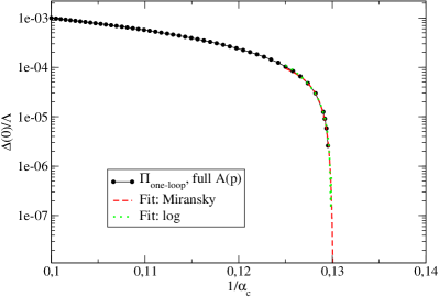
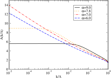
Figure 1: Left: fermion mass function at zero momentum over the inverse coupling, $1/\alpha$, together with two fits for values of the coupling close to the critical one, see text for details. Right: momentum dependence of the Fermi velocity dressing function, exemplified for the couplings $\alpha=6.0,7.0,7.8$ and $\alpha=9.0$, below and above the corresponding critical coupling $\alpha_{c}\approx 7.65(5)$, respectively. Note the logarithmic infrared divergence in the results for $\alpha=6.0,7.0$, whereas for $\alpha=7.8,9.0$ this infrared divergence is screened by the dynamically generated mass. All results are for $N_{f}=2$ here, see text for further details.

Having performed the bifurcation analysis which is appropriate precisely at the critical coupling, we now return to the original system of coupled (nonlinear) integral equations for the fermion propagator, Eqs. (3.4) and (3.5). To illustrate the potential effects of a large $A$-function, here we focus on the frequency dependent RPA Coulomb interaction with the one-loop photon polarization function of Eq. (3.2). Explicitly, the equations then read (with $z$ now as given in (3.7), and $g=\alpha_{\varepsilon}N_{f}\pi/4$ as before):

$$A(p)=1+\frac{\alpha_{\varepsilon}}{2\pi^{2}}\frac{1}{p}\int_{0}^{\Lambda}dk\,k\int_{0}^{\pi}d\theta\frac{\cos\theta}{\sqrt{p^{2}+k^{2}-2\,p\,k\,\cos\theta}}\frac{A(k)}{\sqrt{A^{2}(k)+\frac{\Delta^{2}(k)}{k^{2}v_{F}^{2}}}}J(z,g)\,,$$ (3.16)

$$\Delta(p)=m+\frac{\alpha_{\varepsilon}}{2\pi^{2}}\int_{0}^{\Lambda}dk\int_{0}^{\pi}d\theta\frac{1}{\sqrt{p^{2}+k^{2}-2\,p\,k\,\cos\theta}}\frac{\Delta(k)}{\sqrt{A^{2}(k)+\frac{\Delta^{2}(k)}{k^{2}v_{F}^{2}}}}J(z,g)\,,$$ (3.17)

where we have also included a small bare mass $m$ via the tree-level propagator in the gap equation which acts as an external field for explicitly breaking the extended $U(2N_{f})$ flavor symmetry of the low-energy theory down to $U(N_{f})\times U(N_{f})$ as discussed below.

In the nonlinear case, the critical coupling is obtained from evaluating the numerically determined mass function at zero momentum, in the chiral limit $m=0$, which serves as an order parameter for chiral symmetry breaking together with an extrapolation towards the critical point using appropriate fit functions. Our numerical results together with the fits are shown in the left diagram of Fig. 1. Numerically, we seem to find an exponential decrease of the order parameter close to the critical coupling indicating Miransky scaling similar to the case of ordinary QED₃ Miransky and Yamawaki (1997); Fischer et al. (2004); Braun et al. (2011). Indeed, a corresponding fit of the Miransky type form

$$\Delta(0)/\Lambda=a_{0}\exp\left(\frac{a_{1}}{\sqrt{\frac{1}{\alpha_{c}}-\frac{1}{\alpha}}}\right)$$ (3.18)

delivers excellent results with the parameters $a_{0}=6.4\times 10^{-4}$, $a_{1}=-0.138$ and a critical coupling of $\alpha_{c}=7.68$. However, we also note that the fit form

$$\Delta(0)/\Lambda=\frac{|\alpha-\alpha_{c}|}{\left[\ln\left(\frac{a}{\alpha-\alpha_{c}}\right)\right]^{3}}$$ (3.19)

extracted from analytical results using angular approximation Gusynin works equally well with the parameter $a=345061$ and $\alpha_{c}=7.70$. Both values for the critical coupling obtained in this way are within the range $\alpha_{c}\approx 7.65(5)$ obtained from bifurcation analysis in the last subsection.

To demonstrate the effects of the dynamical mass generation, we show in the right panel of Fig. 1 our numerical results for the Fermi velocity renormalization function at the couplings $\alpha=6$ and $\alpha=7$ as well as $\alpha=7.8$ and $\alpha=9$, below and above the critical coupling $\alpha_{c}$. We notice that in the symmetric phase the selfconsistent numerical solution for $A(p)$ contains a logarithmic divergence at $p^{2}\rightarrow 0$ as in the GW approximation Popovici et al. (2012b). The slope of this logarithmic increase grows with $\alpha$ until the logarithmic infrared divergence gets suppressed due to the dynamical generation of a mass gap when the broken phase is reached such that $A(p)$ approaches a finite value for $\alpha>\alpha_{c}$ in the infrared. While a logarithmic behavior with further increasing slope persists for a certain range of intermediate momenta also in the broken phase above $\alpha_{c}$, the saturation value in the infrared decreases with $\alpha$ from there on, and the momentum scale for this saturation hence increases. From an experimental point of view, the function $A$ plays a very important role, as the Fermi velocity enters the mass function, and many other graphene observables. In fact, recent measurements Elias et al. (2012) provide evidence that the spectrum of suspended graphene is indeed approximately logarithmic instead of linear near charge-neutrality. This logarithmic increase would eventually invalidate the instantaneous Coulomb approximation for the electron interactions in graphene as pointed out in González et al. (1994) already. Phenomenologically, on the other hand, the smallest momenta reached in experiments are limited by the finite size of realistic graphene sheets. For those one observes an increase of the Fermi velocity by a factor (e.g. of the order of three in Elias et al. (2012)). With our present results for the semimetal phase it would typically take sheets that are larger by several orders of magnitude to increase this logarithmic Fermi velocity renormalization factor from 3 to say 10. With the bare $v_{F}/c\approx 1/300$ this would still justify the instantaneous approximation with $Z=1$, as explained below Eq. (3.3), reasonably well.

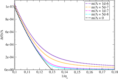
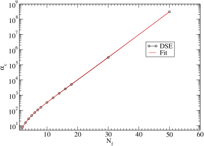
Figure 2: Left: Mass dependence of the order parameter for $N_{f}=2$. Right: Large $N_{f}$ dependence of the critical coupling.

In order to study explicit symmetry breaking effects we have also determined the zero-momentum limit of the mass function for a range of bare fermion masses $m$. The corresponding results are plotted as a family of functions over the inverse coupling in the left panel of Fig. 2. The general pattern is similar to the one seen in the lattice simulations Drut and Lähde (2009). The critical scaling is quite different, however. While infinite volume extrapolations of lattice results have provided evidence of a second order phase transition with associated critical exponents, here we observe the typical Miransky scaling of QED₃ in the continuum approach as mentioned above and discussed in more detail in Ref. Gamayun et al. (2010). Consequently, the magnetic scaling of the order parameter with the mass at the critical coupling is different from that in Drut and Lähde (2009). Whether the infinite volume and chiral limit extrapolations are reliable in such a case is not clear to us.

The explicit symmetry breaking by $m\not=0$ could be due to a staggered chemical potential with opposite signs on the two sublattices as induced by a sublattice-dependent substrate, for example. It would then be a seed for site-centered charge-density wave formation and as such break parity. There are other Dirac mass terms which lead to the same general breaking pattern of the extended flavor symmetry, $U(2N_{f})\to U(N_{f})\times U(N_{f})$, but rather correspond to bond-ordered phases Hou et al. (2007), however. The main difference is whether the residual $U(N_{f})\times U(N_{f})$ mixes the two Dirac points or not Gusynin et al. (2007); Mesterhazy et al. (2012). This can not be distinguished on the level of the gap equation because it depends on the particular choice of the basis used for the reducible four-dimensional representation of the $\gamma$-matrices which we did not have to specify in the derivation of Eq. (3.17).

Finally, let us shortly comment on the dependence of the critical coupling on the number of flavors $N_{f}$. The corresponding curve displayed in the right panel of Fig. 2 can be fitted with an expression of the form

$$f(N_{f})=12.7\,e^{\frac{N_{f}}{3}\sqrt{\frac{N_{fc}}{N_{fc}-N_{f}}}}-14.4\,N_{f}^{0.25}$$ (3.20)

from which we may read off a value for the critical number of (pseudo)fermion species of about $N_{fc}\sim 1200$ for which the critical coupling diverges. While this particular number is certainly not reliable for the reasons discussed above, the general finding of the very existence of a finite value for $N_{fc}$ would confirm a conjecture of Son in Ref. Son (2007). It remains to be seen, however, whether this result survives a selfconsistent treatment of the particle-hole polarization function.

4 Summary and outlook

In this study we have determined critical couplings for the chiral phase transition from the fermion Dyson-Schwinger equation (DSE) with long-range Coulomb interactions in a low-energy model for monolayer graphene at half filling. As compared to previous DSE studies of this model we have for the first time dynamically included a non-trivial Fermi velocity dressing function in our selfconsistent solutions for the fermion propagator. We have thereby compared the effects of static as well as fully frequency-dependent Lindhard screening with the bare Coulomb interaction. In all three cases, the selfconsistent inclusion of the non-trivial Fermi velocity dressing function had dramatic effects, indicating that a substantial renormalization of the Fermi velocity should occur at strong coupling in agreement with experimental evidence from cyclotron-mass measurements in suspended graphene Elias et al. (2012). At the same time, such large Fermi velocity renormalizations also indicate that RPA Coulomb interactions with one-loop polarization function considerably overestimate the screening effects. Whether the screening is nevertheless strong enough for suspended graphene to remain in the semimetal phase remains to be seen from a fully dynamical inclusion of the particle-hole polarization in a simultaneous solution of both, the fermion and the Coulomb photon DSEs in the future.

Including the running Fermi velocity renormalization function, here we obtained $\alpha_{c}\approx 1.22$ for the critical coupling of the semimetal-insulator transition without screening as compared to $\alpha_{c}\approx 7.7$ with the fully frequency-dependent Lindhard screening in the RPA Coulomb interaction. We have argued that a selfconsistent treatment of the particle-hole polarization should lead to a critical coupling between these two extremes with an expected tendency towards values closer to the lower bound. This leaves open the possibility that the critical coupling is larger than the bare coupling $\alpha_{0}=2.16$ for suspended graphene. Quite likely, however, additional screening from the electron states in the $\sigma$ bands of graphene might have to be included in a more realistic calculation to achieve this Wehling et al. (2011).

Although our study is indicative, a number of caveats remain. First of all we need to include the particle-hole polarization effects dynamically and selfconsistently to study their effect on $\alpha_{c}$. When comparing with lattice results it will also be important to take finite volume effects into account. Finally, when comparing with experiment, other type of interactions such as four-fermi couplings might also be important and need to be included in the model. First important steps in this direction have been discussed in Gamayun et al. (2010); Mesterhazy et al. (2012).

Acknowledgments

We are grateful to V. P. Gusynin for pointing out numerical inaccuracies in a previous version of the manuscript and for sending us his private notes on analytical solutions of some of the equations. We would like to thank P. Buividovich, D. Mesterhazy, M. Ulybyshev, D. Smith, S. Strauss and the late M. Polikarpov for helpful discussions. This work was supported by the Deutsche Forschungsgemeinschaft within SFB 634, by the Helmholtz Young Investigator Group No. VH-NG-332, and by the European Commission, FP7-PEOPLE-2009-RG, No. 249203.

References

- Novoselov et al. (2004) K. S. Novoselov, A. K. Geim, S. V. Morozov, D. Jiang, Y. Zhang, S. V. Dubonos, I. V. Grigorieva, and A. A. Firsov, Science 306, 666 (2004), eprint arXiv:cond-mat/0410550.
- Novoselov et al. (2005) K. S. Novoselov, A. K. Geim, S. V. Morozov, D. Jiang, M. I. Katsnelson, I. V. Grigorieva, S. V. Dubonos, and A. A. Firsov, Nature (London) 438, 197 (2005), eprint arXiv:cond-mat/0509330.
- Gusynin and Sharapov (2005) V. P. Gusynin and S. G. Sharapov, Physical Review Letters 95, 146801 (2005), eprint arXiv:cond-mat/0506575.
- Zhang et al. (2005) Y. Zhang, Y.-W. Tan, H. L. Stormer, and P. Kim, Nature 438, 201 (2005), eprint arXiv:cond-mat/0509355.
- Katsnelson et al. (2006) M. I. Katsnelson, K. S. Novoselov, and A. K. Geim, Nature Physics 2, 620 (2006), eprint arXiv:cond-mat/0604323.
- Cheianov and Fal’Ko (2006) V. V. Cheianov and V. I. Fal’Ko, Phys. Rev. B 74, 041403 (2006), eprint arXiv:cond-mat/0603624.
- Rozhkov et al. (2011) A. V. Rozhkov, G. Giavaras, Y. P. Bliokh, V. Freilikher, and F. Nori, Physics Reports 503, 77 (2011), eprint 1104.2183.
- Kotov et al. (2008) V. N. Kotov, B. Uchoa, and A. H. Castro Neto, Phys. Rev. B 78, 035119 (2008), eprint 0706.2185.
- Castro Neto et al. (2009) A. Castro Neto, F. Guinea, N. Peres, K. Novoselov, and A. Geim, Rev.Mod.Phys. 81, 109 (2009).
- Peres (2010) N. M. R. Peres, Reviews of Modern Physics 82, 2673 (2010), eprint 1007.2849.
- Kotov et al. (2012) V. N. Kotov, B. Uchoa, V. M. Pereira, A. C. Neto, and F. Guinea, Rev.Mod.Phys. 84, 1067 (2012), eprint 1012.3484.
- Wallace (1947) P. R. Wallace, Phys. Rev. 71, 622 (1947).
- Slonczewski and Weiss (1958) J. C. Slonczewski and P. R. Weiss, Physical Review 109, 272 (1958).
- Dietz et al. (2013) B. Dietz, M. Miski-Oglu, N. Pietralla, A. Richter, L. von Smekal, et al. (2013), eprint 1304.4764.
- Hou et al. (2007) C.-Y. Hou, C. Chamon, and C. Mudry, Phys.Rev.Lett. 98, 186809 (2007), eprint cond-mat/0609740.
- Jackiw and Pi (2007) R. Jackiw and S.-Y. Pi, Physical Review Letters 98, 266402 (2007), eprint arXiv:cond-mat/0701760.
- Oliveira et al. (2011) O. Oliveira, C. E. Cordeiro, A. Delfino, W. de Paula, and T. Frederico, Phys. Rev. B83, 155419 (2011), eprint 1012.4612.
- Popovici et al. (2012a) C. Popovici, O. Oliveira, W. de Paula, and T. Frederico, Phys.Rev. B85, 235424 (2012a), eprint 1202.3115.
- Cortijo and Vozmediano (2007) A. Cortijo and M. A. Vozmediano, Nucl.Phys. B763, 293 (2007), eprint cond-mat/0612374.
- Pachos and Stone (2007) J. K. Pachos and M. Stone, Int.J.Mod.Phys. B21, 5113 (2007), eprint cond-mat/0607394.
- Vozmediano et al. (2010) M. Vozmediano, M. Katsnelson, and F. Guinea, Phys. Rept. 496, 109 (2010).
- Gamayun et al. (2010) O. Gamayun, E. Gorbar, and V. Gusynin, Phys.Rev. B81, 075429 (2010), eprint 0911.4878.
- Mesterhazy et al. (2012) D. Mesterhazy, J. Berges, and L. von Smekal, Phys. Rev. B86, 245431 (2012), eprint 1207.4054.
- Janssen and Gies (2012) L. Janssen and H. Gies, Phys.Rev. D86, 105007 (2012), eprint 1208.3327.
- Elias et al. (2012) D. C. Elias, R. V. Gorbachev, A. S. Mayorov, S. V. Morozov, A. A. Zhukov, P. Blake, L. A. Ponomarenko, I. V. Grigorieva, K. S. Novoselov, F. Guinea, et al., Nature Physics 8, 172 (2012).
- Bostwick et al. (2009) A. Bostwick, J. L. McChesney, K. V. Emtsev, T. Seyller, K. Horn, S. D. Kevan, and E. Rotenberg, Phys. Rev. Lett. 103, 056404 (2009).
- Khveshchenko (2009) D. V. Khveshchenko, Journal of Physics Condensed Matter 21, 075303 (2009), eprint 0807.0676.
- Vafek and Case (2008) O. Vafek and M. J. Case, Phys. Rev. B 77, 033410 (2008), eprint 0710.2907.
- Drut and Lähde (2009) J. E. Drut and T. A. Lähde, Phys. Rev. B 79, 165425 (2009), eprint 0901.0584.
- Buividovich and Polikarpov (2012) P. Buividovich and M. Polikarpov (2012), eprint 1206.0619.
- Wehling et al. (2011) T. O. Wehling, E. Şaşıoğlu, C. Friedrich, A. I. Lichtenstein, M. I. Katsnelson, and S. Blügel, Phys. Rev. Lett. 106, 236805 (2011), URL http://link.aps.org/doi/10.1103/PhysRevLett.106.236805.
- Ulybyshev et al. (2013) M. Ulybyshev, P. Buividovich, M. Katsnelson, and M. Polikarpov (2013), eprint 1304.3660.
- Sorella and Tosatti (1992) S. Sorella and E. Tosatti, Europhys. Lett. 19, 699 (1992).
- Herbut (2006) I. F. Herbut, Phys. Rev. Lett. 97, 146401 (2006), eprint arXiv:cond-mat/0606195.
- Honerkamp (2008) C. Honerkamp, Phys. Rev. Lett. 100, 146404 (2008), URL http://link.aps.org/doi/10.1103/PhysRevLett.100.146404.
- Meng et al. (2010) Z. Y. Meng, T. C. Lang, S. Wessel, F. F. Assaad, and A. Muramatsu, Nature 464, 847 (2010), URL http://www.nature.com/nature/journal/v464/n7290/suppinfo/nature08942_S1.html.
- Raghu et al. (2008) S. Raghu, X.-L. Qi, C. Honerkamp, and S.-C. Zhang, Phys. Rev. Lett. 100, 156401 (2008), URL http://link.aps.org/doi/10.1103/PhysRevLett.100.156401.
- González et al. (1994) J. González, F. Guinea, and M. A. H. Vozmediano, Nuclear Physics B 424, 595 (1994), eprint arXiv:hep-th/9311105.
- Alkofer and von Smekal (2001) R. Alkofer and L. von Smekal, Phys. Rept. 353, 281 (2001), eprint hep-ph/0007355.
- Maris and Roberts (2003) P. Maris and C. D. Roberts, Int.J.Mod.Phys. E12, 297 (2003), eprint nucl-th/0301049.
- Fischer (2006) C. S. Fischer, J. Phys. G32, R253 (2006), eprint hep-ph/0605173.
- Maris (1995) P. Maris, Phys.Rev. D52, 6087 (1995), eprint hep-ph/9508323.
- Fischer et al. (2004) C. S. Fischer, R. Alkofer, T. Dahm, and P. Maris, Phys. Rev. D 70, 073007 (2004), eprint arXiv:hep-ph/0407104.
- Bonnet et al. (2011) J. A. Bonnet, C. S. Fischer, and R. Williams, Phys. Rev. B84, 024520 (2011), eprint 1103.1578.
- Bonnet and Fischer (2012) J. A. Bonnet and C. S. Fischer, Phys. Lett. B718, 532 (2012), eprint 1201.6139.
- Popovici (2013) C. Popovici, Mod.Phys.Lett. A28, 1330006 (2013), eprint 1302.5642.
- Popovici et al. (2012b) C. Popovici, C. Fischer, and L. von Smekal, PoS ConfinementX, 269 (2012b), eprint 1302.2365.
- González et al. (1999) J. González, F. Guinea, and M. A. H. Vozmediano, Phys. Rev. B 59, 2474 (1999), eprint arXiv:cond-mat/9807130.
- Khveshchenko (2001) D. V. Khveshchenko, Physical Review Letters 87, 246802 (2001), eprint arXiv:cond-mat/0101306.
- Gorbar et al. (2001) E. V. Gorbar, V. P. Gusynin, and V. A. Miransky, Phys. Rev. D 64, 105028 (2001), eprint arXiv:hep-ph/0105059.
- Gorbar et al. (2002) E. V. Gorbar, V. P. Gusynin, V. A. Miransky, and I. A. Shovkovy, Phys. Rev. B 66, 045108 (2002), eprint arXiv:cond-mat/0202422.
- Atkinson et al. (1994) D. Atkinson, J. C. R. Bloch, V. P. Gusynin, M. R. Pennington, and M. Reenders, Physics Letters B 329, 117 (1994).
- Hoffman (2001) J. Hoffman, Numerical Methods for Engineers and Scientists (McGraw-Hill Book company, New York, 2001).
- Gusynin and Reenders (2003) V. Gusynin and M. Reenders, Phys.Rev. D68, 025017 (2003), eprint hep-ph/0304302.
- Goecke et al. (2009) T. Goecke, C. S. Fischer, and R. Williams, Phys.Rev. B79, 064513 (2009), eprint 0811.1887.
- (56) V. Gusynin, private communication.
- Gamayun et al. (2009) O. V. Gamayun, E. V. Gorbar, and V. P. Gusynin, Phys. Rev. B 80, 165429 (2009), URL http://link.aps.org/doi/10.1103/PhysRevB.80.165429.
- Miransky and Yamawaki (1997) V. Miransky and K. Yamawaki, Phys.Rev. D55, 5051 (1997), eprint hep-th/9611142.
- Braun et al. (2011) J. Braun, C. S. Fischer, and H. Gies, Phys.Rev. D84, 034045 (2011), eprint 1012.4279.
- Gusynin et al. (2007) V. P. Gusynin, S. G. Sharapov, and J. P. Carbotte, International Journal of Modern Physics B 21, 4611 (2007), eprint 0706.3016.
- Son (2007) D. T. Son, Phys. Rev. B 75, 235423 (2007).