Magnetic properties of a long, thin-walled ferromagnetic nanotube

Abstract

We consider magnetic properties of a long, thin-walled ferromagnetic nanotube. We assume that the tube consists of isotropic homogeneous magnet whose spins interact via the exchange energy, the dipole-dipole interaction energy, and also interact with an external field via Zeeman energy. Possible stable states are the parallel state with the magnetization along the axis of the tube, and the vortex state with the magnetization along azimuthal direction. For a given material, which of them has lower energy depends on the value $\gamma=R^{2}d/(L\lambda_{x}^{2})$, where $R$ is the radius of the tube, $d$ is its thickness, $L$ is its length and $\lambda_{x}$ is an intrinsic scale of length characterizing the ration of exchange and dipolar interaction. At $\gamma<1$ the parallel state wins, otherwise the vortex state is stable. A domain wall in the middle of the tube is always energy unfavorable, but it can exist as a metastable structure. Near the ends of a tube magnetized parallel to the axis a half-domain structure transforming gradually the parallel magnetization to a vortex just at the edge of the tube is energy favorable. We also consider the equilibrium magnetization textures in an external magnetic field either parallel or perpendicular to the tube. Finally, magnetic fields produced by a nanotube and an array of tubes is analyzed.

I INTRODUCTION

Magnetic nanomaterials play an important role in applications as elements of memory and magnetic sensors and switches as it was demonstrated by Nobel prize 2007 to Fert and Grünberg for their invention of antiferromagnetic spin valve. The task of further miniaturization of magnetic devices and creation of configurations providing a controllable magnetic field is extremely important for nanophysics and technology. Experimenters and technologists have already created nanomagnets in different shapes – disks disk , rings ring , wires nanowire , etc. Among these new nanomaterials the nanotubes, as compared to solid wires, have inner voids that reduce the density of materials and makes them easier to float in solutions, a desirable property in biotechnology. equilibrium states The inner hollow itself can be used for capturing large biomolecules. chemistry Besides, as magnetic materials, they are free of vortex cores, which makes the vortex state more stable than that of nanowires. This makes nanotubes more suitable as candidates for elements of memory for computers and as a tool for creation of superconductors with high critical fields. Several methods have been used to synthesize nanotubes: electrodeposition Nielsch 3 ; electrodeposition , atomic layer deposition ALD , hydrogen reduction hydrogen reduction . Ferromagnetic materials used for formation of nanotubes include Ni, ALD , Co Nielsch 3 ; ALD , FePt hydrogen reduction , $\mathrm{Fe_{3}O_{4}}$ hydrogen reduction .

Together with the experimental progress, theoretical calculations and numerical simulations for nanotubes were performed extensively, dealing with the stable states phase diagrams ; equilibrium states , switching behavior reversal modes , hysteresis loop equilibrium states ; angular dependence and properties of domain walls (both static reversal modes or dynamic dynamic DW ). In Ref. phase diagrams the authors calculated numerically and partly analytically energy of the parallel state and the vortex state as function of the dimensions of the tube and material constants. Phase diagrams were drawn in terms of linear dimensions of the tube. In Ref. equilibrium states the authors have shown that the parallel magnetization turns into a vortex-like one at the edge of the tube.

The purpose of our work is to give an analytical description of the magnetic tubes (MT) properties employing small parameters characterizing their geometry: the ratios $d/R$ and $R/L$. In the experimentally realized MT the first ratio was in the range of $10^{-3}$ and the second one varied between $10^{-2}$ and $10^{-1}$. The analytical approach allows as to construct the complete phase diagram of the MT in the space of geometric parameters and external magnetic field. We establish analytical criteria for the appearance and disappearance of different topological magnetic configuration, topological defects and field-induced magnetic textures. We also calculate the magnetic field produced by the tubes.

II THE MODEL

We take into account the magnetic interactions of two kinds: the exchange interaction and the dipolar interaction. The total energy of a MT is:

$$E = E_{exch}+E_{dip}$$ (1)

$$= -J\sum_{<\mathbf{x},\mathbf{x^{\prime}}>}\mathbf{S_{x}}\cdot\mathbf{S_{x^{\prime}}}+\frac{\mu_{0}}{4\pi}(g\mu_{B})^{2}\sum_{\mathbf{x},\mathbf{x^{\prime}},\mathbf{x}\neq\mathbf{x^{\prime}}}\frac{\mathbf{S_{x}}\cdot\mathbf{S_{x^{\prime}}}-3(\mathbf{S_{x}}\cdot\mathbf{\hat{r}})(\mathbf{S_{x^{\prime}}}\cdot\mathbf{\hat{r}})}{r^{3}}.$$

Here $\mathbf{S_{x}}$ is the spin vector at position $\mathbf{x}$, $J$ is the exchange constant, $\mathbf{\hat{r}}$ is the unit vector from position $\mathbf{x}$ to $\mathbf{x^{\prime}}$, $<\mathbf{x},\mathbf{x^{\prime}}>$ means summation over all nearest pairs, and $r=|\mathbf{r}|=|\mathbf{x}-\mathbf{x^{\prime}}|$. griffiths Further we use the International System of units. Another often considered contribution to the total energy, the crystal anisotropy is not included here. This is appropriate when the material is a polycrystal with large number of randomly orientated grains like permalloy. Experimenters Nielsch 3 indicate that the size of a single-crystal grain in their nanotubes is about 1nm. We do not know how strong is the exchange interaction between the grains. In our calculations we assume that it is the same as in the bulk single crystal.

We accept an approximation of classical continuous field $\mathbf{m(x)}$ for the magnetic order parameter with the constraint $\mathbf{m}^{2}(\mathbf{x})=1$. The magnetization at the point $\mathbf{x}$ of the space is equal to $M_{0}\mathbf{m}(\mathbf{x})$. The saturation magnetization $M_{0}$ is assumed to be dependent on temperature, but independent of the point $\mathbf{x}$ of the space. In this approximation aharoni the exchange energy reads:

$$E_{exch}=A\int d^{3}x(\mathbf{\nabla m(x)})^{2},$$ (2)

where $A=\frac{1}{6}Jns^{2}Za^{2}$, $n$ is the density of magnetic atoms, $s$ is the magnitude of their spin, $(\mathbf{\nabla m(x)})^{2}=(\nabla m_{x}(\mathbf{x}))^{2}+(\nabla m_{y}(\mathbf{x}))^{2}+(\nabla m_{z}(\mathbf{x}))^{2}$, $n$ is the number of magnetic atoms per unit volume, $a$ is the distance between two nearest atoms, $Z$ is the coordination number.

There are several equivalent expressions for the dipolar energy:

$$E_{dip}=\frac{1}{2}\frac{\mu_{0}}{4\pi}M_{0}^{2}\int d^{3}xd^{3}x^{\prime}\frac{\mathbf{m(x)}\cdot\mathbf{m(x^{\prime})}-3(\mathbf{m(x)}\cdot\mathbf{\hat{r}})(\mathbf{m(x^{\prime})}\cdot\mathbf{\hat{r}})}{r^{3}},$$ (3a)

$$E_{dip}=\frac{1}{2}\frac{\mu_{0}}{4\pi}M_{0}^{2}\int d^{3}xd^{3}x^{\prime}(\mathbf{m(x)}\cdot\mathbf{\nabla_{x}})(\mathbf{m(x^{\prime})}\cdot\mathbf{\nabla_{x^{\prime}}})\frac{1}{r},$$ (3b)

$$E_{dip} = \frac{1}{2}\frac{\mu_{0}}{4\pi}M_{0}^{2}\left[\int dAdA^{\prime}\frac{\sigma_{M}(\mathbf{x})\sigma_{M}(\mathbf{x^{\prime}})}{r}+2\int dAd^{3}x^{\prime}\frac{\sigma_{M}(\mathbf{x})\rho_{M}(\mathbf{x^{\prime}})}{r}\right.$$ (3c)

$$\left.+\int d^{3}xd^{3}x^{\prime}\frac{\rho_{M}(\mathbf{x})\rho_{M}(\mathbf{x^{\prime}})}{r}\right].$$

The integration denoted by $\int dA,\int dA^{\prime}$ proceeds over the surfaces of the magnet, the integration denoted as $\int d^{3}x$ goes over its volume. The value $\sigma_{M}(\mathbf{x})=\mathbf{m(x)}\cdot\mathbf{n}$ is the “surface magnetic charge density” and $\rho_{M}(\mathbf{x})=-\nabla_{x}\cdot\mathbf{m(x)}$ is the “volume magnetic charge density”. Eq. (3c) is a form analogous to the energy of electric charges interacting via Coulomb forces. This analogy allows to use results well-known in electrostatics. An important consequence of this analogy is that the dipolar energy is non-negative, since the electrostatic energy is equal to the integral of the square of the electric field. Eq. (3c) provides a clear electrostatic visualization of the dipolar interaction. Eq. (3b) may occur more convenient for specific calculations. A system of magnetic charges is always neutral.

III STABLE STATES

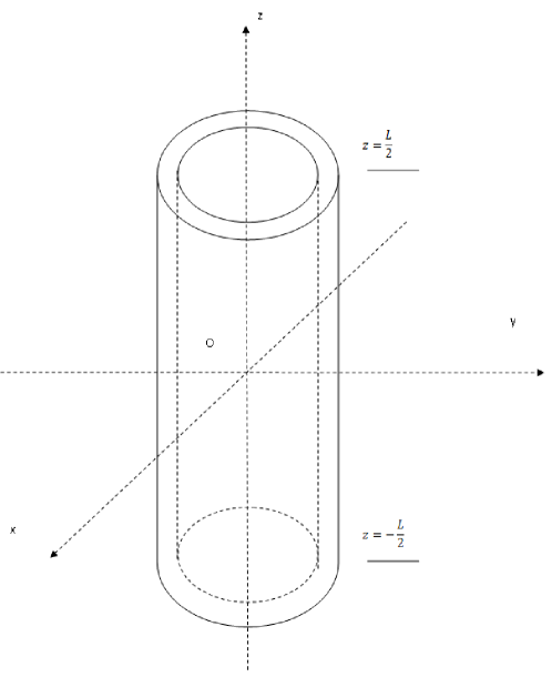
Figure 1: Geometry of a tube, with two edges located at $z=L/2$ and $z=-L/2$.

We consider a cylindrical tube located between $z=-\frac{L}{2}$ and $z=\frac{L}{2}$, as shown in Fig. 1, with the radius $R$, thickness $d$, and length $L$. We assume $d\ll R\ll L$. This research was initially stimulated by a new material fabricated experimentally by Dr. Wenhao Wu and his group at Texas A&M University: an array of nickel nanotubes in alumina with dimensions approximately $R=150nm$, $d=30nm$ and $L=60\mu m$. For these nanotubes the condition $R\ll L$ is well satisfied, while the condition $d\ll R$ is relatively not so well satisfied. Besides, $R^{2}\ll dL$ is also well satisfied. In earlier experiments [1-9] all three strong inequalities were satisfied.

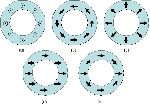
Figure 2: Pictorial characteristic of different magnetization distributions: (a) parallel; (b) vortex; (c) radial; (d) transverse; (e) onion.

Natural candidates to the state with the lowest energy are the most symmetric magnetic configurations: the parallel state: $\mathbf{m(x)}=\hat{z}$, and the vortex state: $\mathbf{m(x)}=\hat{\phi}$. We denote azimuthal angle as $\phi$; the symbol $\mathbf{m(x)}=\hat{\phi}$ denotes the unit vector in azimuthal direction. Each of these states is two-fold degenerate due to time reversal invariance. We also consider two other, less symmetric states: the transverse state: $\mathbf{m(x)}=\hat{x}$, and the so-called onion state. According to Ref. bland review , the onion state (see Fig. 2), becomes stable in ferromagnetic rings in some range of parameters. Here we consider its analogue for a tube. These two kinds of states occur to be stable magnetic configuration in the transverse magnetic field.

In the parallel state, $\mathbf{\nabla m(x)}=0$, $\rho_{M}(\mathbf{x})=0$, $\sigma_{M}(\mathbf{x})=\pm 1$ for $z=\pm\frac{L}{2}$, respectively, and $\sigma_{M}(\mathbf{x})=0$ elsewhere. The exchange energy is zero. The dipolar energy consists of three parts: the self-energies of the two edges and the energy of interaction between them two. Since $R\ll L$, the latter term is much smaller than the former two and further we neglect it. The distance $r$ between two points with the cylindrical coordinates $(\rho,\phi,z)$ and $(\rho^{\prime},\phi^{\prime},z^{\prime})$ belonging to a MT satisfying the inequality $d\ll R$ reads: $r\approx\sqrt{(\rho-\rho^{\prime})^{2}+2R^{2}[1-\cos(\phi-\phi^{\prime})]+(z-z^{\prime})^{2}}$. Each self-energy term after integration over $\phi$ and $\phi^{\prime}$ is reduced to an integral of the complete elliptic integral of the first kind $K(k)$ where $k=\sqrt{\frac{4\rho\rho^{\prime}}{(\rho+\rho^{\prime})^{2}}}$. The condition $d\ll R$ allows us to use the approximation $K(k)\thickapprox 2\log 2-\frac{1}{2}\log(1-k^{2})$ since $k$ is close to 1. In this approximation the integration over $\rho$ and $\rho^{\prime}$ is straightforward leading to the result for the self-energy of each edge: $E(\textrm{edge})=\frac{1}{2}\mu_{0}M_{0}^{2}Rd^{2}(\log\frac{8R}{d}+\frac{3}{2})$. Thus, in the limit of long thin MT the total energy of the parallel state is: $E_{P}=\mu_{0}M_{0}^{2}Rd^{2}(\log\frac{8R}{d}+\frac{3}{2})$. It does not depend on the tube length $L$.

Different magnetic configurations and results of similar calculations of exchange and dipolar energy for them are summarized in Table 1.

Table 1. Magnetic configurations and energies.

state magnetization vector exchange energy dipolar energy parallel(P) $\hat{z}$ 0 $\mu_{0}M_{0}^{2}Rd^{2}(\log\frac{8R}{d}+\frac{3}{2})$ vortex(V) $\hat{\phi}$ $2\pi A\frac{Ld}{R}$ 0 radial(R) $\hat{\rho}$ $2\pi A\frac{Ld}{R}$ $\pi\mu_{0}M_{0}^{2}RdL$ transverse(T) $\hat{x}$ 0 $\frac{\pi}{2}\mu_{0}M_{0}^{2}RdL$ onion(O) $\hat{x}\cos(a\sin 2\phi)-\hat{y}\sin(a\sin 2\phi)$ $4\pi A\frac{Ld}{R}a^{2}$ $\frac{\pi}{2}\mu_{0}M_{0}^{2}RdL[1-J_{1}(2a)]$

While other configurations are trivial, some comments on the onion configuration are necessary. We seek for a variational distribution of magnetization that satisfies following requirements: magnetization must be parallel to magnetic field (in the direction $\hat{x}$) at $\phi=0,\pm\pi/2,\pi$ and it does not depend on the coordinate $r$ in a narrow ring. A simplest vector field satisfying these requirements has a form $\mathbf{m}(\phi)=\hat{x}\cos\theta(\phi)+\hat{y}\sin\theta(\phi)$ with $\theta(\phi)=-a\sin(2\phi)$, where $a$ is a variational parameter. Its value should minimize the total energy. ($a=0$ corresponds to the transverse state.) As it is seen from the last line of the Table 1, the minimum energy corresponds to a largest maximum of the Bessel function $J_{1}(2a)$=0.583. It corresponds to $a=0.92$, and $E_{O}=\frac{\pi}{2}\mu_{0}M_{0}^{2}RdL*0.418$. It is smaller than $E_{T}$. Since the exchange energy is quadratic in $a$, the minimum of the total onion configuration energy shifts to a value of $a$ between $0$ and $0.92$. It is easy to check that the difference of the total onion energy and transverse energy at $a=0$ is zero, whereas the derivative of this difference over $a$ is negative. Therefore, its value in the minimum of the onion energy is negative. In other words, the onion is energy preferable to the transverse configuration. If $R\gg\lambda_{x}$, where $\lambda_{x}=\sqrt{A/(\mu_{0}M_{0}^{2})}$ is the so-called exchange length, the exchange interaction of the onion configuration is much smaller than the dipolar term, so $a$ is very close to $0.92$. A typical value of $\lambda_{x}$ is several nanometers. exchange length

The parallel and transverse states have zero exchange energy; the vortex state has zero dipolar energy. In the absence of magnetic field the hierarchy of energy scales is as follows: $E_{T}>E_{O}\gg E_{P}$, so the transverse and the onion states are not stable. Only the parallel or the vortex states are stable. Which of these two states is more favorable depends on the ratio:

$$\gamma=\frac{E_{P}}{E_{V}}=\frac{R^{2}d}{2\pi\lambda_{x}^{2}L}\left(\log\frac{8R}{d}+\frac{3}{2}\right).$$ (4)

At $\gamma<1$ the parallel states wins, in opposite case the vortex state wins. The logarithmic factor varies comparatively slowly, and $\gamma$ depends mainly on the combination $\frac{R^{2}d}{L}$. We see that large $L$ favors the parallel magnetization, while large $R$ and $d$ favor the vortex magnetization. It is convenient to introduce dimensionless lengths $R^{\prime}=\frac{R}{\lambda_{x}}$, $d^{\prime}=\frac{d}{\lambda_{x}}$, $L^{\prime}=\frac{L}{\lambda_{x}}$. Then $\gamma$ can be expressed as

$$\gamma=\frac{R^{\prime 2}d^{\prime}}{2\pi L^{\prime}}\left(\log\frac{8R^{\prime}}{d^{\prime}}+\frac{3}{2}\right).$$ (5)

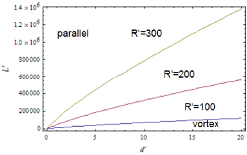
Figure 3: Phase boundaries between the parallel state and the vortex state. The region above a transition line corresponds to the parallel state. The three transition lines from bottom to top corresponds to $R^{\prime}=100,200$ and 300 respectively.

Equation $\gamma=1$ determines the transition line between the two states. In Fig. 3 three transition lines in the $(L^{\prime},d^{\prime})$ plane at fixed values of $R^{\prime}$ are depicted.

The external field can stabilize the transverse or the onion state. This problem will be analyzed in section V.2.

IV DOMAIN WALLS

Let us consider a tube with one domain wall (DW) far from the edges. Calculations in this section are performed in the limit $L\rightarrow\infty$.

In a DW between two opposite parallel states $\mathbf{m(x)}=\pm\hat{z}$, the magnetization can rotate either in the plane $(\hat{z},\hat{\phi})$, or in the plane $(\hat{z},\hat{\rho})$. The corresponding two types of DWs have magnetization $\mathbf{m(x)}=\hat{z}\cos\theta+\hat{\phi}\sin\theta$ or $\mathbf{m(x)}=\hat{z}\cos\theta+\hat{\rho}\sin\theta$ where $\theta$ depends on $z$. These two types of domain walls will be denoted as P1 and P2, respectively. Similarly, in a DW between two opposite vortex states $\mathbf{m(x)}=\pm\hat{\phi}$ the magnetization rotates either in the plane $(\hat{\phi},\hat{z})$, or in the plane $(\hat{\phi},\hat{\rho})$. The corresponding expressions for magnetization in these DWs are: $\mathbf{m(x)}=\hat{\phi}\cos\theta+\hat{z}\sin\theta$ and $\mathbf{m(x)}=\hat{\phi}\cos\theta+\hat{\rho}\sin\theta$. We denote these two types of domain walls as V1 and V2, respectively. We will take the trial function for $\theta$ to be

$$\theta(z)=2\arctan e^{\frac{z}{l}},$$ (6)

where $l$ is the DW width. Plugging the expressions for magnetization with $\theta(z)$ defined by Eq. (6) into the energy functionals (2) and (3c) and calculating the integrals, we arrive at the DW energy (the energy of a tube with a DW minus the energy of the corresponding single domain state) for the four types of domain walls:

$$E_{P1}=C(\frac{1}{\eta}+\eta+\lambda f_{1}(\eta)),$$ (7)

$$E_{P2}=C(\frac{1}{\eta}+\eta+\lambda f_{1}(\eta)+\kappa\eta^{2}f_{2}(\eta)),$$ (8)

$$E_{V1}=C(\frac{1}{\eta}-\eta+\lambda f_{3}(\eta)),$$ (9)

$$E_{V2}=C(\frac{1}{\eta}+\kappa\eta^{2}f_{2}(\eta)),$$ (10)

where we have introduced the dimensionless DW width $\eta=\frac{l}{R}$ and dimensionless coordinate $\zeta=\frac{z}{l}$. Other notations are as follows: $C=4\pi Ad$, $\lambda=\frac{\mu_{0}M_{0}^{2}Rd}{8\pi A}=\frac{Rd}{8\pi\lambda_{x}^{2}}$, $\kappa=\frac{\mu_{0}M_{0}^{2}R^{3}}{4\pi Ad}=\frac{R^{3}}{4\pi\lambda_{x}^{2}d}$,

$$f_{1}(\eta)=\int d\zeta d\zeta^{\prime}kK(k)\mathrm{sech}^{2}\zeta\mathrm{sech}^{2}\zeta^{\prime},\;$$

$$f_{2}(\eta)=\int d\zeta d\zeta^{\prime}[kK(k)-k_{d}K(k_{d})]\mathrm{sech}\zeta\mathrm{sech}\zeta^{\prime},$$

$$f_{3}(\eta)=\int d\zeta d\zeta^{\prime}kK(k)\tanh\zeta\mathrm{sech}\zeta\tanh\zeta^{\prime}\mathrm{sech}\zeta^{\prime},$$

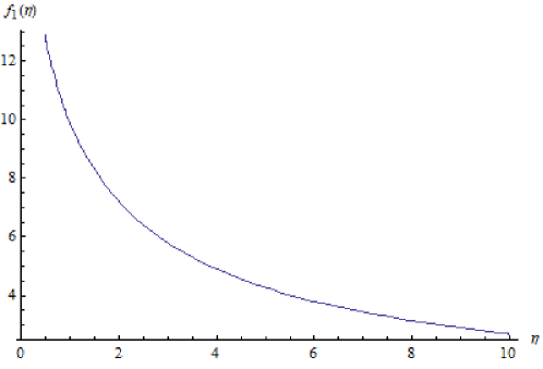
(a)

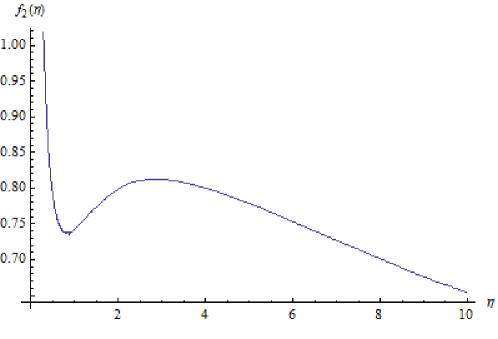
(b)

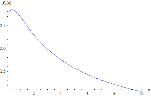
(c)

Figure 4: Plot of the functions: (a)$f_{1}(\eta)$; (b)$f_{2}(\eta)$; (c)$f_{3}(\eta)$.

where $k=\left[1+\frac{1}{4}\eta^{2}(\zeta-\zeta^{\prime})^{2}\right]^{-1/2}$, $k_{d}=\left[1+\frac{d^{2}}{4R^{2}}+\frac{1}{4}\eta^{2}(\zeta-\zeta^{\prime})^{2}\right]^{-1/2}$, and $K(k)$ is the complete elliptic integral of the first kind. The function $f_{1}(\eta)$ decreases monotonically as $\eta$ increases, $f_{3}(\eta)$ has a maximum at $\eta=0.37$, and $f_{2}(\eta)$ has a maximum that depends on the value of $\frac{d}{R}$ (for $\frac{d}{R}=0.1$ it is at $\eta=2.9$). All functions $f_{i}(\eta)$, $i=1,2,3$ are positive for any $\eta$ and turn into zero at $\eta\rightarrow\infty$. They are plotted in Fig. 4.

From the positivity of $f_{i}(\eta)$, it follows that $E_{P1}$, $E_{P2}$ and $E_{V2}$ are positive since each term in Eqs. (7), (8) and (10) is positive. For the V1 case, there is one negative term $-C\eta$. Any solution (if it does exist) of the equation for extremum of the energy (9), i.e. $\lambda f_{3}^{\prime}(\eta)=\eta^{-2}+1$, can only lie between 0 and 0.37 since only in this region is $f_{3}^{\prime}(\eta)$ positive. In the same interval the difference $1/\eta-\eta$ is positive and therefore the energy $E_{V2}$ is also positive. Thus, if the DW energy has a minimum, it must be at a value of $\eta$ smaller than 0.37. Since it was already proved that $E_{V1}>0$ for $\eta<1$, we conclude that inner domain walls are never stable. However, they can exist as metastable states. For the P1 DW and $\lambda=0$ (negligible dipolar interaction), the minimum is realized at $\eta=1$, i.e. at $l=R$. So, if only the exchange energy is considered, the DW width is equal to the radius of the tube. If the dipolar energy is included, the minimum shifts to $l>R$. This looks reasonable, since the volume charge $\rho_{M}(\mathbf{x})=\sin\theta\partial_{z}\theta$ inside the DW has the same sign throughout the wall and it tends to spread out the DW width to reduce the dipolar energy. The energy $E_{P2}$ differs from $E_{P1}$ only by a positive term $\kappa\eta^{2}f_{2}(\eta)$. Thus, the P2 DW is always less favorable than the P1 one. For a V1 DW, numerical calculations show that $E_{V1}$ has a minimum only at $\lambda>97.109$. The value of $\eta$ realizing the minimum of energy at $\lambda=97.109$ is $0.2467$. It monotonically decreases with increasing $\lambda$. Thus, the metastable V1 DW exists at $\lambda>97.109$ and its width is smaller than $0.2467R$.

Summarizing, under our assumptions no stable DW exist in the middle of the magnetic tube, but they can exist as metastable configurations. It is well known that dipolar interaction generates a stripe domain structure in a bulk rectangular ferromagnetic slab. It does not happen in a thin-walled long magnetic tube. The domains in it can not appear as equilibrium state, but only as a result of the growth process from two or more nuclei. However, the edge DW regularly appear. (see section VI)

V MAGNETIC STRUCTURES IN EXTERNAL MAGNETIC FIELD

The external magnetic field $\mathbf{H}$ interacts with magnetization via the Zeeman energy:

$$E_{Z}=-\mu_{0}M_{0}\int d^{3}x\mathbf{m(x)}\cdot\mathbf{H}.$$ (11)

If the external field is directed along $z$-axis (parallel field), the azimuthal symmetry is still retained. A field of any other direction destroys this symmetry. We will first consider the parallel field and then the field along a transverse direction.

V.1 Parallel field

First we analyze the action of the parallel magnetic field $\mathbf{H}=H\hat{z}$ onto the vortex state. The magnetization acquires a finite $z$-component and can be written as

$$\mathbf{m(x)}=\hat{\phi}\cos\theta+\hat{z}\sin\theta,$$ (12)

where $\theta$ is a function of $H$ only. At magnetic field $H$ varying from zero to some critical value $H_{c}$, the angle $\theta$ changes from zero to $\pm\pi/2$ and the configuration changes continuously from the vortex to parallel state. Eq. (11) implies that $E_{Z}=-\mu_{0}M_{0}\int d^{3}xH\sin\theta=-2\pi\mu_{0}M_{0}RdLH\sin\theta\triangleq-E_{Z0}\sin\theta$, where $E_{Z0}=2\pi\mu_{0}M_{0}RdLH$ is the absolute value of $E_{Z}$ for the parallel states. The exchange energy of the state (12) is equal to the energy of the vortex state at zero field multiplied by the factor $\cos^{2}\theta$. The dipolar energy of the configuration (12) is equal to the dipolar energy of the parallel state at $H=0$ multiplied by $\sin^{2}\theta$. The total energy of configuration (12) is

$$E(\theta) = E_{V}\cos^{2}\theta+E_{P}\sin^{2}\theta-E_{Z0}\sin\theta$$ (13)

$$= (E_{P}-E_{V})\left[\sin\theta-\frac{E_{Z0}}{2(E_{P}-E_{V})}\right]^{2}+\frac{E_{Z0}^{2}}{4(E_{P}-E_{V})}+E_{V}.$$

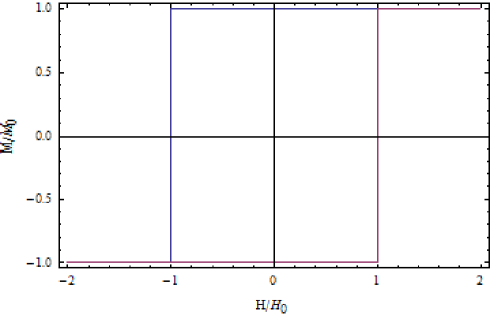
(b)

Figure 5: (a) The dependence of magnetization in a parallel magnetic field at $E_{P}>E_{V}$. Note the absence of hysteresis. (b) Hysteresis in a parallel external field at $E_{P}<E_{V}$.

If $E_{P}>E_{V}$ (the tube is in the vortex state at $h=0$) and $E_{Z0}<2\left(E_{P}-E_{V}\right)$, then $\sin\theta=\frac{E_{Z0}}{2(E_{P}-E_{V})}$ corresponds to the minimum of energy, and the equilibrium energy is between the energies of V and P states. The plot of the net magnetization $M=M_{0}\sin\theta$ vs. $H$ is shown in Fig. 5(a). The critical field at which the parallel state is reached is $H_{C}=\frac{E_{P}-E_{V}}{\pi\mu_{0}M_{0}RdL}$. If $E_{P}<E_{V}$ (the tube is in the parallel state at $H=0$), then $\sin\theta=\frac{E_{Z0}}{2(E_{P}-E_{V})}$ corresponds to the maximum of energy that realizes an energy barrier between the two parallel states. The plot $M$ vs. $H$ displays a rectangular hysteresis loop with the coercive force equal to $H_{c}$, as shown in Fig. 5(b).

This feature reminds the Stoner-Wohlfarth model Stoner-Wohlfarth . The reason of the hysteresis in the Stoner-Wolfarth model is the crystal field anisotropy, i.e. spin-orbit interaction. In magnetic tubes the geometry is anisotropic. At $E_{P}>E_{V}$ and magnetic field along the axis of the tube, the geometric anisotropy keeps the component of magnetization perpendicular to the field and provides a continuous transition at a critical field to completely parallel magnetization. In the opposite case $E_{P},E_{V}$ and initial magnetization antiparallel to the field, an intrinsic hysteresis appears in the absence of the spin orbit interaction due to the exchange and dipolar forces. At magnetic field $\pm H_{c}$ the magnetization flips.

We considered the mechanism of a coherent magnetization flip resulting in a comparatively large coercive force. Other mechanisms were proposed in equilibrium states ; reversal modes . The only mechanism relevant to the limit of a long thin tube is the propagation of a vortex domain wall between two opposite parallel configuration. The vortex DW propagation is favorable if the dipolar energy dominates. in Ref. equilibrium states , Vortex DW propagation is also described and argued to be closely related to the half vortex DWs at the tube ends for one parallel state. Notice that in equilibrium states they also have an almost rectangular-shaped hysteresis loop. While transverse DW propagation is favorable if the exchange energy dominates such that a transverse DW has lower energy than a vortex DW reversal modes . We do not take pinning into account. It is expected that if pinning is included the hysteresis loop will have a larger coercive force.

V.2 Infinite magnetic tube in a transverse magnetic field

Now we consider the transverse magnetic field applied to a tube that was initially in a vortex state. Let the field be in the $x$ direction: $\mathbf{H}=H\hat{x}$. The field violates the azimuthal symmetry. The direction of magnetization in the transverse field deviates from $\hat{\phi}$. We assume that $\mathbf{m(x)}$ depends only on $\phi$ and it does not have $z$-component:

$$\mathbf{m(x)}=\hat{\phi}\cos\theta(\phi)+\hat{\rho}\sin\theta(\phi).$$ (14)

At $H=0$ the vortex state $\mathbf{m(x)}=\hat{\phi}$ has minimal energy. At very large $H$ the transverse state $\mathbf{m(x)}=\hat{x}$ is energy favorable. These two states are topologically different: the former has the winding number 1 while the latter has the winding number 0. The transition from one of them to another can not proceed continuously. It should be a first order transition at a critical value of magnetic field accompanying with the discontinuity of net magnetization $M$. It was reported in bland review that such a transition indeed happens in a ferromagnetic ring: at a critical transverse field, the magnetization transits from the vortex state to the onion state. We will show that the magnetization in a tube also follows this scenario. The exact transition behavior to the onion state is still unknown. It may include the escape of the magnetization from $xy$-plane. Below we compare the energy of the modified vortex state and that of the onion state to determine the critical field of the transition.

The energy of the onion state is the sum of the onion energy $E_{O}$ at zero magnetic field and the Zeeman energy $E_{Z}=-\mu_{0}M_{0}\int d^{3}xH\cos\theta=-\pi\mu_{0}M_{0}HRdl[1+J_{0}(2a)]$. (We again use the trial function $\theta(\phi)=-a\sin(2\phi)$.) The total onion energy is:

$$E_{O}(a,H) = 4\pi A\frac{Ld}{R}a^{2}+\frac{\pi}{2}\mu_{0}M_{0}^{2}RdL[1-J_{1}(2a)]-\pi\mu_{0}M_{0}HRdl[1+J_{0}(2a)]$$ (15)

$$= 4\pi A\frac{Ld}{R}\left\{a^{2}+\frac{R^{2}}{8\lambda_{x}^{2}}\left[1-J_{1}(2a)-2\frac{H}{M_{0}}\left[1+J_{0}(2a)\right]\right]\right\}.$$

This energy should be minimized with respect to $a$. Let the equilibrium value of $a$ be $a_{0}$. It is physically obvious that the equilibrium value of variational parameter $a_{0}$ monotonically decreases with $H$ increasing and reaches zero at $H=\infty$. Therefore, it cannot be larger than $0.92$ – the maximum value of $a_{0}$ at zero field.

The vortex state also changes in the presence of magnetic field. The local magnetization approaches to the direction of magnetic field, so that the vortex configuration acquires a non-zero total magnetic moment. We describe this changes by a trial function:

$$\mathbf{m(x)}=\frac{\hat{\phi}+b\hat{x}}{\sqrt{1+b^{2}-2b\sin{\phi}}}=\hat{\phi}\frac{1-b\sin\phi}{\sqrt{1+b^{2}-2b\sin{\phi}}}+\hat{\rho}\frac{b\cos\phi}{\sqrt{1+b^{2}-2b\sin{\phi}}},$$ (16)

where $b$ is a non-negative parameter which does not depend on $\phi$. At $b=0$ the trial configuration turns into the genuine vortex state and at $b=\infty$ it turns into the transverse state. The energy of the modified vortex state reads:

$$E_{MV}(b,H) = \pi A\frac{Ld}{R}\frac{2-b^{2}}{1-b^{2}}+\frac{\pi}{4}\mu_{0}M_{0}^{2}RdLb^{2}-\frac{2\mu_{0}M_{0}HRdl}{b}[(1+b)E(k)-(1-b)K(k)]$$ (17)

$$= \pi A\frac{Ld}{R}\left\{\frac{2-b^{2}}{1-b^{2}}+\frac{R^{2}}{\lambda_{x}^{2}}\left[\frac{b^{2}}{4}-\frac{2}{\pi}\frac{H}{M_{0}}\left[\frac{b+1}{b}E(k)-\frac{1-b}{b}K(k)\right]\right]\right\},$$

where $k=\frac{\sqrt{4b}}{1+b}$; $K(k)$ and $E(k)$ are complete elliptic integrals of the first and the second kind, respectively. The energy (17) should be minimized with respect to $b$. Let the equilibrium value of $b$ be $b_{0}$.

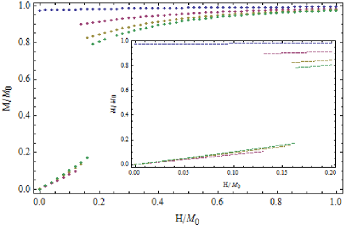
Figure 6: (Color Online) Plot of magnetization vs. magnetic field (in units $M_{0}$) in a transverse field for 4 values of the parameter $R/\lambda=\infty,8,4,2$ (from bottom to top). The inset shows $M$ vs. $H$ in small $H$ region. $H_{C}/M_{0}$ for $R/\lambda=\infty,8,4,2$ are 0.163, 0.159 and 0.131, respectively.

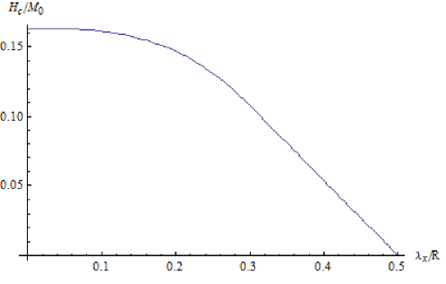
Figure 7: Plot of the critical field $H_{C}$ vs. $\lambda_{x}/R$.

Given $a_{0}$ and $b_{0}$, the phase transition condition $E_{MV}(b_{0})=E_{O}(a_{0})$ determines the critical field $H_{C}$ (the field at which transition between the onion and the modified vortex state takes place). The basic equations of the Table 1 show that, at $\frac{R}{\lambda_{x}}<2$, the transverse state has lower energy than the vortex state at zero field, and the more at any non-zero field. Thus, the transition proceeds only at $\frac{R}{\lambda_{x}}>2$. Fig. 6 presents the plots of $M$ vs. $H$ (both divided by $M_{0}$) for 4 different values of $\frac{R}{\lambda_{x}}=\infty,8,4,2$. The corresponding values of the critical field $\frac{H_{C}}{M_{0}}$ are $0.163$, $0.159$ and $0.131$. At $\frac{R}{\lambda_{x}}=2$ the tube is in the onion state at zero field. Fig. 7 presents the critical field $H_{c}$ v.s. $\lambda_{x}$. Note that these results does not depend on the ratio $d/R$, although we still have to be in the $\frac{d}{R}\ll 1$ limit.

VI THE EDGE MAGNETIC TEXTURES

Although we have proved that the DW in the middle of a tube is never energy favorable, it occurs that a finite tube in the parallel state has a vortex-like magnetization at its edges. The transitional texture from the parallel to vortex magnetization can be imagined as half of the P1 type DW. We will call such a texture the edge DW (EDW). Such a structure was found theoretically in Ref. equilibrium states where it is called a mixed state. The EDW weakens the stray magnetic field near the edges and reduces the dipolar energy. From the magnetic charge point of view, in the EDW the surface charge at the edges is spread out into the volume, so that the total charge remains invariant. When the reduction of dipolar energy exceeds the increase of the exchange energy, the state with the EDW becomes stable. Since the total length $L$ is much larger than the width $l$ of the EDW, the magnetization in the tube beyond the two EDW does not change.

Let us consider the EDW in more details. We consider an semi-infinite tube whose axis coincides with the positive half-axis $z$. We also assume that the stable magnetic configuration is parallel at $z\rightarrow\infty$. The magnetization at arbitrary $z$ can be represented as $\mathbf{m(x)}=\hat{z}\cos\theta+\hat{\phi}\sin\theta$, where $\theta$ is a function of $z$ satisfying the boundary conditions $\theta(\infty)=\pi$, while $\theta(0)$ is a variational parameter. If either it occurs not equal to $\pi/2$ or $\frac{d\theta}{dz}\neq 0$, it means that the surface magnetic charge does not vanish completely. To take in account this effect, we employ the trial function:

$$\theta(z)=2\arctan e^{\frac{z+z_{0}}{l}},$$ (18)

where $z_{0}=\log\tan\frac{\theta_{0}}{2}$. This trial function is reasonable also in the presence of external magnetic field parallel to the axis. Therefore, we will perform variational calculations for arbitrary magnetic field $H$. For this purpose we need to complement the Hamiltonian by the Zeeman energy: $E_{Z}=-\mu_{0}M_{0}\int d^{3}x\mathbf{H}\cdot(\mathbf{m(x)}+\hat{z})=\mu_{0}M_{0}H\int d^{3}x(1+\cos\theta)$ where $\mathbf{H}=-H\hat{z}$. Calculations similar to the case of the P1 type DW result in the following energy $E_{E}$ of the edge configuration:

$$E_{E} = \frac{1}{2}C\{(1-\tanh\zeta_{0})(\frac{1}{\eta}+\eta)$$ (19)

$$+\lambda_{E}\left[2\tanh\zeta_{0}g(\eta,\zeta_{0})+f(\eta,\zeta_{0})+(\tanh^{2}\zeta_{0}-1)\log(\frac{8R}{d}+\frac{3}{2})\right]$$

$$+\mu\eta\left[\log(2\cosh\zeta_{0})-\zeta_{0}\right]\},$$

where $\lambda_{E}=2\lambda$, $\mu=\frac{\mu_{0}M_{0}HR^{2}}{A}=\frac{R^{2}}{\lambda_{x}^{2}}\frac{H}{M_{0}}$, $\zeta_{0}=\frac{z_{0}}{l}$,

$$f(\eta,\zeta_{0})=\int_{0}^{\infty}\int_{0}^{\infty}d\zeta d\zeta^{\prime}kK(k)\mathrm{sech}^{2}(\zeta+\zeta_{0})\mathrm{sech}^{2}(\zeta^{\prime}+\zeta_{0}),$$

$$g(\eta,\zeta_{0})=\int_{0}^{\infty}d\zeta kK(k)|_{\zeta^{\prime}=0}\mathrm{sech}^{2}(\zeta+\zeta_{0})\mathrm{sech}^{2}(\zeta^{\prime}+\zeta_{0}).$$

Other notations are the same as in section IV.

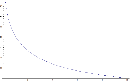
Figure 8: Plot of the function $f(\eta,0)$.

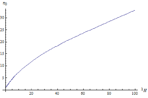
Figure 9: Plot of $\eta_{0}$ vs. $\lambda_{E}$ for $d/R=0.1$.

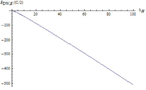
Figure 10: Plot of $E_{DW,E}$ vs. $\lambda_{E}$ at $d/R=0.1$.

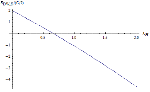
Figure 11: Plot of $E_{DW,E}$ vs. $\lambda_{E}$ at $d/R=0.1$, small $\lambda_{E}$ region. $E_{DW,E}=0$ at about $\lambda_{E}=0.66$.

Let us start with the analysis of the EDW at zero magnetic field. The EDW is stable if $E_{E}<0$. In turn this condition implies a necessary condition of the EDW stability $f(\eta,0)<\log\frac{8R}{d}+\frac{3}{2}$. In Fig. 8 we plot the graph of $f(\eta,0)$ vs. $\eta$ for $\eta\in[0.1,10]$. The necessary condition of the EDW stability is satisfied for $\eta>1$. Since $f(\eta,0)$ monotonically decreases, the value $\eta=\eta_{0}$ which minimizes $E_{E}$ is also located in the region $\eta>1$. Thus, the stable EDW has the width $l>R$. Fig. 9 presents the graph of $\eta_{0}$ vs. $\lambda_{E}$. It shows that, at $\lambda_{E}$ increasing from zero, $\eta_{0}$ increases from 1 monotonically. Asymptotically at large $\lambda_{E}$, the dependence of $\eta$ on $\lambda_{E}$ becomes linear. Figs. 10 and 11 present the graphs of $E_{E}/(C/2)$ vs. $\lambda_{E}$ for large and small $\lambda_{E}$, respectively. The calculations were performed at a fixed value $\frac{d}{R}=0.1$. Fig. 11 shows that the energy becomes negative at $\lambda_{E}>0.66$. Since $\lambda_{E}=2\lambda=\frac{Rd}{4\pi\lambda_{x}^{2}}$, the criteria of the EDW stability at $\frac{d}{R}=0.1$ is $Rd>2.64\pi\lambda_{x}^{2}$, i.e. $R>9.1\lambda_{x}$. For typical figures $R\sim 100nm$, $d\sim 10nm$ and $\lambda_{x}$ several nanometers, the stability condition is readily satisfied.

The value $\zeta_{0}$ at zero magnetic field is not zero, but it is rather small (about 0.04). However it grows with increasing magnetic field as it is shown in the Table 2. The same table displays the equilibrium values parameter $\eta$ and energy of the edge texture as function of magnetic field ($\mu$) at $d/R=0.1$ and $\lambda_{E}=50$. The Table 2 also shows the dependence of the equilibrium value of $\eta$ on $\mu$. Magnetic field reduces $\eta$ to values less than one, i.e. it narrows the edge domain wall width to $l<R$. The last column of the Table 2 shows that the energy of the EDW becomes positive at $\mu>427$. The field $H$ corresponding to $\mu=427$ is $0.0680M_{0}$. Thus, in a tube with $\frac{d}{R}=0.1$ and $\lambda_{E}=50$, the EDW vanishes at a critical field $H_{E}=0.0680M_{0}$.

Note that the critical field $H_{E}$ here is obtained by equalizing the energy of the parallel and the EDW state. If we want to examine the nucleation of EDW in more detail, we should perform stability analyses for both the parallel and the EDW state, and we are likely to get a hysteresis between the two states. Nevertheless the field $H_{E}$ here remains a good estimate of the transition field between these two states.

Table 2. Energies and parameters of EDW in external field at $d/R=0.1$ and $\lambda_{E}=50$.

$\mu$ $\eta$ $\zeta_{0}$ $E_{DW,E}/(C/2)$ 0 21.7496 0.0385034 -242.641 100 0.792432 0.108815 -75.4210 200 0.408263 0.139860 -39.8710 300 0.278412 0.168046 -18.9154 400 0.229659 0.230356 -3.68804 500 0.213332 0.285309 9.35049 600 0.206421 0.320128 21.4643

VII STRAY MAGNETIC FIELD

Now we calculate the field produced by the nanotube. The field at a point $\mathbf{x}$ outside the tube reads:

$$\mathbf{B(x)}=-\frac{\mu_{0}}{4\pi}M_{0}\nabla\phi(\mathbf{x})=-\frac{\mu_{0}}{4\pi}M_{0}\mathbf{\nabla_{x}}[\int d^{3}x^{\prime}\frac{\rho_{M}(\mathbf{x^{\prime}})}{r}+\int dA^{\prime}\frac{\sigma_{M}(\mathbf{x^{\prime}})}{r}].$$ (20)

For a vortex state, $\rho_{M}(\mathbf{x})=\sigma_{M}(\mathbf{x})=0$ everywhere, so that $\mathbf{B(x)}=0$ everywhere outside the material. In the parallel state $\mathbf{m(x)}=\hat{z}$, the only charges are $\sigma_{M}(\mathbf{x})=1$ at $z=\frac{L}{2}$ and $\sigma_{M}(\mathbf{x})=-1$ at $z=-\frac{L}{2}$. If the observation point is not too close to the tube, it is possible to neglect the change of radius $\rho^{\prime}$ replacing it by $R$. Then integration over the radius is reduced to multiplication by $d$. Integration over $\phi$ leads to complete elliptic integrals. We are mostly interested in the $z$ component of the field, which is:

$$B_{z}(\mathbf{x})=\frac{\mu_{0}}{\pi}M_{0}Rd\left[\frac{(z-z^{\prime})E(\sqrt{\frac{4\rho R}{(\rho+R)^{2}+(z-z^{\prime})^{2}}})}{\sqrt{(\rho+R)^{2}+(z-z^{\prime})^{2}}[(\rho-R)^{2}+(z-z^{\prime})^{2}]}\right]_{z=-\frac{L}{2}}^{z=\frac{L}{2}}.$$ (21)

For an observation point separated from the tube by a distance much larger than $R$, the field is well approximated by the field of two point magnetic charges. In regions near the edges magnetic field changes rapidly. Let us consider for example a region $z-\frac{L}{2}\ll L$. In a part of this region the finiteness of the radius $R$ is important. The contribution to the field from the edge $z=-\frac{L}{2}$ can be ignored. Introducing dimensionless variables $h=\frac{z-\frac{L}{2}}{R}$ and $r=\frac{\rho}{R}$, we find

$$B_{z}(\mathbf{x})=\frac{\mu_{0}M_{0}d}{\pi R}\frac{hE(\sqrt{\frac{4r}{(r+1)^{2}+h^{2}}})}{\sqrt{(r+1)^{2}+h^{2}}[(r-1)^{2}+h^{2}]}.$$ (22)

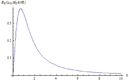
Figure 12: Plot of $B_{z}(\mathbf{x})$ (divided by $\frac{\mu_{0}M_{0}d}{2R}$) vs. $z$, which presents the field along the $z-$axis.

Eq. (23) becomes simpler on the $z-$axis: $B_{z}(0,z)=\frac{\mu_{0}M_{0}d}{2R}\frac{h}{(1+h^{2})^{\frac{3}{2}}}$. By symmetry the field on the $z-$axis must be parallel to the $z-$axis. Fig. 12 presents the graph of $B_{z}(0,z)$ divided by $\frac{\mu_{0}M_{0}d}{2R}$ vs. $h$. It starts from zero, reaches a maximum equal to $\frac{2\sqrt{3}}{9}$ at $h=\frac{\sqrt{2}}{2}$. and then decreases to zero. Thus, the maximum field along the $z$ axis locates at $\frac{2\sqrt{3}}{9}R\approx 0.385R$ above the upper edge. Fig. 13(a) presents the graphs of $B_{z}(\mathbf{x})$ in units $\frac{\mu_{0}M_{0}d}{\pi R}$ vs. $r$ at different $h$. Note the maxima of $B_{z}(\mathbf{x})$ at $r\approx 1$, i.e. at $\rho\approx R$. The smaller is $h$, the larger and sharper is the maximum. It is well-known singularity of the field of homogeneously charged ring.

What about field produced by an EDW state? The EDW near the $z=\frac{L}{2}$ edge is described like before: $\mathbf{m(x)}=\hat{z}\cos\theta+\hat{\phi}\sin\theta$, where

$$\theta(z)=2\arctan e^{\frac{z-\frac{L}{2}-z_{0}}{l}}.$$ (23)

Using Eq. (20), the $z-$component of magnetic field at a point $(\rho,\phi,z)$ above the $z=\frac{L}{2}$ edge is:

$$B_{z}(r,h) = \frac{\mu_{0}M_{0}d}{\pi R}[\frac{hE(\sqrt{\frac{4r}{(r+1)^{2}+h^{2}}})}{\sqrt{(r+1)^{2}+h^{2}}[(r-1)^{2}+h^{2}]}\tanh\zeta_{0}$$ (24)

$$+\int_{-\infty}^{0}d\zeta^{\prime}\frac{hE(\sqrt{\frac{4r}{(r+1)^{2}+(h-\eta\zeta^{\prime})^{2}}})}{\sqrt{(r+1)^{2}+(h-\eta\zeta^{\prime})^{2}}[(r-1)^{2}+(h-\eta\zeta^{\prime})^{2}]}\mathrm{sech}^{2}(\zeta^{\prime}-\zeta_{0})],$$

where in addition to $h$ and $r$ we have defined $\eta=l/R$, $\zeta=\frac{z-\frac{L}{2}}{l}$ and $\zeta_{0}=z_{0}/l$. To calculate numerically, we use $\eta=21.7496$ and $\zeta_{0}=0.0385034$ which are values at $d/R=0.1,\lambda_{E}=50$ and zero external field. Fig. 13(b) presents $B_{z}(r,h)$ in units $\frac{\mu_{0}M_{0}d}{\pi R}$ at $h=1/3,2/3$ and 1. Comparing with Fig. 13(a), we see that although peaks remain at $r\approx 1$ they are are more than 10 times lower, and also are more smeared. Thus the EDW reduces the field and smears the singularity (though does not completely remove it).

Now we consider the field produced by a periodic array of tubes. Such an array appears in the experiments employing the template technique, e.g in Nielsch 3 and electrodeposition . Let the infinite array of tubes spread out in the $x-y$ plane forming equilateral triangular lattice (like in the experiment Nielsch 3 ). We assume that all the tubes are in the $\mathbf{m(x)}=\hat{z}$ parallel state. Below we calculate $B_{z}(\mathbf{x})$ near the upper plane of the system $z=\frac{L}{2}$ for the lattice constant $D=3R$ and $2R$. The field is periodic with periodicity of the lattice. It allows us to restrict calculations by one quarter of the elementary cell.

Let us introduce a frame of reference with the $z-$axis parallel to the tube axes and the $x-$axis along one of directions connecting axes of nearest neighboring tubes, i.e. along one of basic vectors of the Bravais lattice. The expression for $B_{z}(\mathbf{x})$ is an infinite sum of the fields produced by a single tube at a particular place, each of them given by Eq. (22) with the position of a tube taking into account. To perform the summation approximately, we calculate exactly the contribution of several nearest tubes and replace the sum over the rest of the tubes by an integral.

Let us start with the field directly on the $z-$axis. We calculate separately the contribution of the 7 nearest tubes and integrate out the contribution of the others. We denote $h=\frac{z-\frac{L}{2}}{R}$ and $\delta=\frac{D}{R}$. The result is:

$${B_{z}(0,0,\frac{L}{2}+hR)}=\frac{\mu_{0}M_{0}d}{\pi R}g(h,\delta),$$ (25)

where

$$g(h,\delta) = \frac{\pi}{2}\frac{h}{(1+h^{2})^{\frac{3}{2}}}+6\frac{hE(\sqrt{\frac{4\delta}{(\delta+1)^{2}+h^{2}}})}{\sqrt{(\delta+1)^{2}+h^{2}}[(\delta-1)^{2}+h^{2}]}$$ (26)

$$+2\pi\frac{2}{\sqrt{3}\delta^{2}}\int_{\sqrt{\frac{7\sqrt{3}}{2\pi}}\delta}^{\infty}\frac{hE(\sqrt{\frac{4r}{(r+1)^{2}+h^{2}}})}{\sqrt{(r+1)^{2}+h^{2}}[(r-1)^{2}+h^{2}]}rdr.$$

The functions $g(h,\delta)$ vs. $h$ at $\delta=3$ and 2 are plotted numerically in Fig. 14. They grow from zero asymptotically to $g(\infty,3)=\frac{2\pi^{2}}{9\sqrt{3}}=1.266$ and $g(\infty,3)=\frac{2\pi^{2}}{4\sqrt{3}}=2.849$. At $h=1$ the fields are already very close to the maxima. The asymptote corresponds to the uniform field produced by an infinite uniformly-charged plane. (Note that at distances larger than $L$ the charges at the plane $z=-\frac{L}{2}$ makes the field zero at infinity.)

For the field other not necessary on the $z-$axis, we calculate separately the contribution of the 12 nearest tubes centered at $(x,y)=(D/2,\sqrt{3}D/2)$, and integrate out the rest. Figs. 15 and 16 are the 3-dim graphs for the function $g(x,y,h,\delta)$ ($B_{z}$ divided by $\frac{\mu_{0}M_{0}d}{\pi R}$) in the region $0<x<D,0<y<D$ for $\delta=3$ and 2 (dense filling), respectively. Both are plotted for $h=1/3,2/3,1$. The ridges lie above the tube edges, as expected. The $\delta=2$ cases in general have stronger fields than the corresponding $\delta=3$ cases. Comparing with Fig. 13(a) we see that the field produced by an array of tubes has a larger strength and varies slower than the field of a single tube.

Again the EDW change the results smearing the field singularities. Another source of deviations from the simplified model considered above is the dipolar interaction between tubes. It tends to establish magnetization in each nearest pair of the tubes oppositely. However, a rather small magnetic field is sufficient to stabilize the parallel orientation of magnetization in the tubes.

VIII CONCLUSIONS

We calculated analytically the exchange and the dipolar energies of different states for a ferromagnetic long, thin-walled nanotube with zero crystal anisotropy. In the approximation of infinitely long tubes at zero external field we have found two possible stable states: the parallel state and the vortex state. Which of them has lower energy depends on the dimensionless ratio $\frac{\mu_{0}M_{0}^{2}R^{2}d}{AL}$. For a long tube with small radius and thickness the parallel state is favored; increasing the radius and thickness it is possible to stabilize the vortex state. For a tube in either of these two states, a domain wall in the middle is proved to be always not energy-favorable. But for the parallel state there can exist a stable half-DW structures at the edges of the tube if the radius and thickness are large enough. In an external field parallel to the tube in the vortex state no hysteresis appears, whereas the tube in the parallel state subject to the same field displays a rectangular hysteresis loop. When a field perpendicular to the tube axis is applied, the vortex state turns into the onion state at a critical field. This transition is accompanied by a jump of the magnetization. We also calculated the stray magnetic field generated by single magnetic tube and the periodic array of the tubes. It displays a singularity near the edges especially in strong external magnetic field. The singularities are partly smeared out by the edge domain walls at external magnetic field decreasing.

(a)

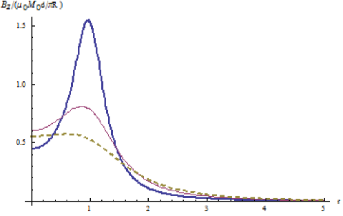
(a)
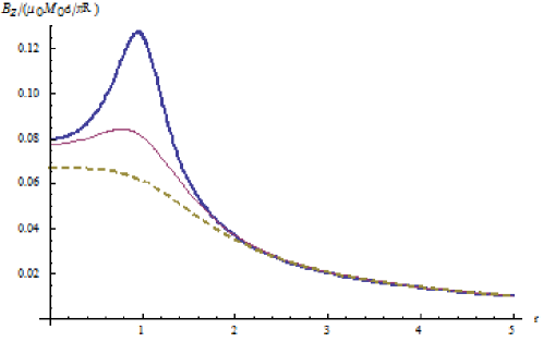
(b)

Figure 13: (Color online) (a) Plot of $B_{z}(\mathbf{x})$ (divided by $\frac{\mu_{0}M_{0}d}{\pi R}$) vs. $r$ at $h=1/3$ (thick), 2/3 (solid), 1(dashed), respectively, for a tube in the parallel state. (b) The same as (a), but for a tube with EDW. The parameters describing the EDW are $\eta=21.7496$ and $\zeta=0.0385034$.

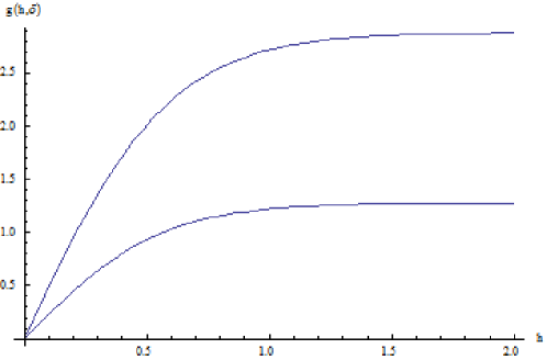
Figure 14: Plot of the function $g(h,\delta)$ (i.e. $B_{z}(\mathbf{x})$ divided by $\frac{\mu_{0}M_{0}d}{\pi R}$) at $\delta=3$ (bottom) and $\delta=2$ (up).

(a)

(b)

(c)

Figure 15: Plot of the function $g_{(}x,y,h,\delta)$ vs. $r$ at $\delta=3$, and at (a) $h=1/3$ (thick); (b) $h=2/3$ (solid); (c) $h=1$(dashed).

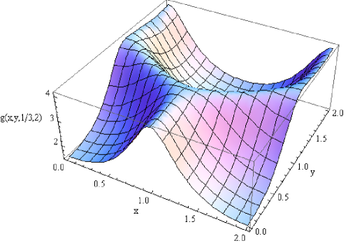
(a)

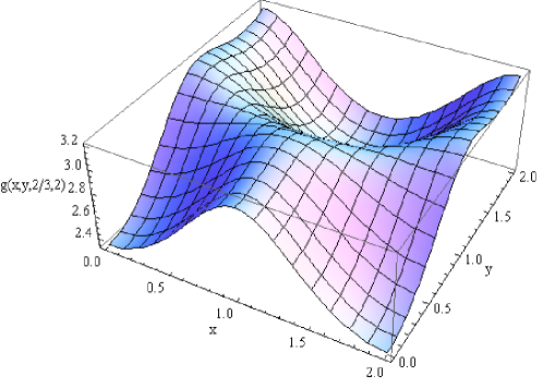
(b)

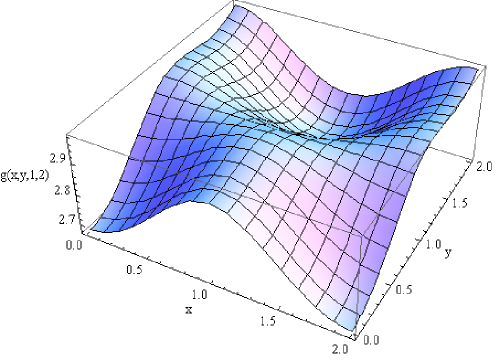
(c)

Figure 16: Same as Fig. 15, but at $\delta=2$.

References

- (1) C.A.F. Vaz, L. Lopez-Diaz, M. Klâui, J.A.C. Bland, T. L. Monchesky, J. Unguris, Z. Cui, Phys. Rev. B 67, 140405 (2003).
- (2) M. Klâui, C.A.F. Vaz, L. Lopez-Diaz and J.A.C. Bland, J. Phys.: Condens. Matter 15, 985 (2003).
- (3) Zuwei Liu, Pai-Chun Chang, Chia-Chi Chang, Evgeniy Galaktionov, Gerd Bergmann, and Jia G. Lu, Phys. Rev. B 80, 214410 (2009).
- (4) P. Landeros, O.J. Suarez, A. Cuchillo, P. Vargas, Phys. Rev. B 79, 024404 (2009).
- (5) S.J. Son, J. Reichel, B. He, M. Schuchman, S.B Lee, J. Am. Chem. Soc. 127, 7316 (2005).
- (6) K. Nielsch, F.J. Castaño, S. Matthias, W. Lee, C.A. Ross, Adv. Eng. Mater. 7, 217 (2005).
- (7) Dongdong Li, Richard S. Thompson, Gerd Bergmann, and Jia G. Lu, Adv. Mater. 20 4575-4578 (2008).
- (8) M. Daub, M. Knez, U. Goesele and K. Nielsch, J. Appl. Phys. 101, 09J111 (2007).
- (9) Y. C. Sui, R. Skomski, K. D. Sorge, and D. J. Sellmyer, J. Appl. Phys. 95, 7151 (2004).
- (10) J. Escrig, P. Landeros, D. Altbir, E.E. Vogel, P. Vargas, J. Magn. Magn. Mater. 308, 233-237 (2007).
- (11) P. Landeros, S. Allende, J. Escrig, E. Salcedo, D. Altbira, E. E. Vogel, Appl. Phys. Lett. 90, 102501 (2007).
- (12) L.D. Landau, E.M. Lifshitz and L.P. Pitaevskii, Electrodynamics of Continuous Media, 2nd ed. (Butterworth, Oxford, 1984).
- (13) J. Escrig, M. Daub, P. Landeros, K. Nielsch, and. D Altbir, Nanotechnology 18, 445706 (2007).
- (14) P. Landeros, and Álvaro S. Núñez, J. Appl. Phys. 108, 033917 (2010).
- (15) D.J. Griffiths,Introduction to Electrodynamics, 3rd ed. (Prentice Hall, New Jersey,1999).
- (16) Gavin S. Abo, Yang-Ki Hong, Jihoon Park, Jaejin Lee, Woncheol Lee, and Byoung-Chul Choi, IEEE Trans. Magn. 49, 3055-3057 (2013).
- (17) A. Aharoni, Introduction to the Theory of Ferromagnetism (Clarendon, Oxford, 1996).
- (18) E.C. Stoner and E.P. Wohlfarth, Phil. Trans. R. Soc. Lond. A 240, 599-642 (1948).
- (19) M. Kläui, C.A.F Vaz, L. Lopez-Diaz and J.A.C Bland, J. Phys.: Condens. Matter, 79, R985 (2003).
(a)
(b)
(c)
(a)
(b)
(a)
(b)
(a)
(b)
(c)
(a)
(b)
(c)