Moments Method for Shell-Model Level Density

Abstract

The modern form of the Moments Method applied to the calculation of the nuclear shell-model level density is explained and examples of the method at work are given. The calculated level density practically exactly coincides with the result of full diagonalization when the latter is feasible. The method provides the pure level density for given spin and parity with spurious center-of-mass excitations subtracted. The presence and interplay of all correlations leads to the results different from those obtained by the mean-field combinatorics.

The long-standing problem of nuclear level density is important both from a theoretical viewpoint as a powerful instrument for studying nuclear structure and for numerous applications. Nuclear technology requires the detailed knowledge of level density, especially in the region around the neutron separation energy. Astrophysical reactions responsible for the nucleosynthesis in the Universe can be understood only if we know the nuclear level density in the Gamow window. The interest to this problem is also connected with the necessity to develop methods of statistical physics and thermodynamics for small mesoscopic systems (complex nuclei, atoms and molecules, nanoscale devices, prototypes of quantum computers).

Application of statistical physics to studies of nuclear properties was started in the early years of nuclear physics by Frenkel [1], Bethe [2, 3] and Landau [4]. Such ideas served as a base for a concept of compound nucleus by Bohr [5]. The review of those ideas and their further development was given in Refs. [6, 7]. At this stage theory of level density and detailed microscopic nuclear theory were growing more or less independently along parallel paths. Their synthesis became possible when the reliable versions of the nuclear shell model were established for several segments of the nuclear chart. Of course, this is related to the modern computational tools.

In this presentation we show the practical way of finding the density of energy levels with fixed exact quantum numbers (spin, parity, isospin projection) for a given shell model Hamiltonian. The method becomes practical because it is avoiding the full diagonalization of prohibitively large matrices. In contrast to popular mean-field approaches [8, 9, 10], all many-body correlations are fully accounted for, albeit in a restricted orbital space. The exact classification of states according to the conserved quantities and therefore the absence of artificial standard spin cut-off parameters is the advantage compared to Monte-Carlo calculations although some of them give relatively good results [11, 12]. Similar problems still may arise in approaches based on statistical spectroscopy [13].

Our method was gradually developed in several publications [14, 15, 16, 17, 18, 19, 20, 21, 22]. A high-performance code for calculating spin- and parity-dependent level density is available via the Computer Physics Communication homepage on Science Direct [23]. Technically we use the Moments method based on statistical spectroscopy [24, 25], the applications are compared to the results obtained with the full diagonalization in the nuclear shell model with effective interactions when such calculations are practically possible [26]. The method is reinforced by the use of the recurrence relations [27, 28, 17] for eliminating spurious contributions.

We start with the shell-model Hamiltonian that contains mean-field single-particle energies in the restricted space and effective two-body interactions (many-body forces can be added without problems although the equations become more cumbersome). The spherical orbitals $|njm\rangle$ are used as a basis, and the counted many-body levels have definite total spin $J$ and parity. A certain distribution of non-interacting particles over orbitals defines a configuration (partition). For each partition $p$, let $D_{\alpha p}$ be the number of many-body states with exact quantum numbers $\{\alpha\}$ including the number of particles, spin, parity, isospin… The diagonal matrix elements of the total (including interaction) Hamiltonian define the energy centroid $E_{\alpha p}$ for the states of class $\alpha$ built in the partition $p$,

$$E_{\alpha p}=\,\frac{1}{D_{\alpha p}}\,{\rm Tr}^{(\alpha p)}\,H.$$ (1)

For each partition we define also the effective width (energy dispersion) $\sigma_{\alpha p}$,

$$\sigma_{\alpha p}^{2}=\,\frac{1}{D_{\alpha p}}\,{\rm Tr}^{(\alpha p)}\,H^{2}-(E_{\alpha p})^{2}.$$ (2)

The contribution of each state to this width, related to the strength function of an unperturbed state fragmented over the exact eigenstates, can be found summing the squares of off-diagonal matrix elements of the full Hamiltonian over a given row of the matrix $H$. Here the interaction between the states of different partitions is fully accounted for. As known from the shell-model experience [26, 29], the centroids of partitions form a smooth sequence, while the widths of individual unperturbed states fluctuate only weakly which can be considered as one of features of quantum chaos (in particular, geometric chaoticity of angular momentum addition [30], that emerges, for a realistic strength of interactions, already at rather low excitation energy). The details of calculating the trace of $H^{2}$ and explanation of the computational algorithm can be found in Ref. [23]; a computational method based on group theory but close in spirit to our approach is presented in Ref. [31].

The set of quantities (1) and (2) forms a foundation of the Moments Method [24]. The level density of each partition is known [32] to be close to Gaussian. The first two moments define it with sufficient precision. The total level density is restored by summing the contributions of the partitions,

$$\rho(E;\alpha)=\sum_{p}D_{\alpha p}G_{\alpha p}(E),$$ (3)

where $G_{\alpha p}(E)$ is a finite range Gaussian with the centroid at $E_{\alpha p}$ counted from the ground state energy; this Gaussian is cut at a distance $\eta\sigma_{\alpha p}$ from the centroid, where $\eta$ is an empirical parameter eliminating the unphysical tails of the Gaussian (there are theoretical arguments confirmed by experience that fix $\eta$ between 2.5 and 3). The ground state energy is to be found independently, for example by the approximate diagonalization in a smaller space and the exponential convergence method [33, 34], where the exponential regime also starts approximately at a distance of 3-4 spreading widths.

The last essential point is exclusion of unphysical states corresponding to the center-of-mass excitation which are present in the shell-model calculations due to cross-shell mixing. If we classify the basis states similarly to the harmonic oscillator field by $N\hbar\omega$ excitations, then for $N=0$ the spurious excitations are absent, $\rho_{{\rm pure}}(E,J,N=0)=\rho_{{\rm calc}}(E,J,N=0)$. With $N=1$ excitations we have to subtract from the shell-model result the states which could be obtained by the action of the center-of-mass vector operator on all states of $N=0$ class,

$$\rho_{{\rm pure}}(E,J,N=1)=\rho_{{\rm calc}}(E,J,N=1)-\sum_{J^{\prime}=J,J\pm 1}\rho_{{\rm calc}}(E,J^{\prime},N=0).$$ (4)

The final result is expressed by a recurrent relation similar to used in [27, 28]:

$$\rho_{{\rm pure}}(E,J,N)=\rho_{{\rm calc}}(E,J,N)-\sum_{K=1}^{N}\sum_{J_{K}=J_{{\rm min}}}^{N,{\rm step}\,2}\sum_{J^{\prime}=|J-J_{K}|}^{J+J_{K}}\rho_{{\rm calc}}(E,J^{\prime},N-K).$$ (5)

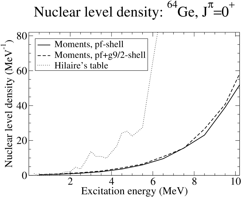
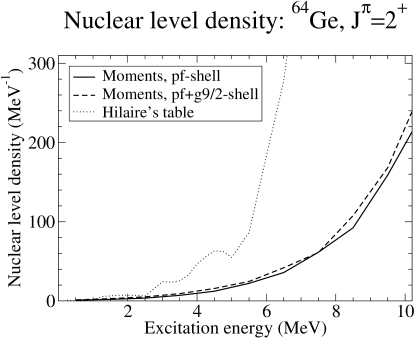
Figure 1: ⁶⁴Ge nuclear level density for $J=0,2$ and positive parity. Solid and dashed lines present calculations by Moments method in $pf$- (calculated with GXPF1A interaction) and $pf+g_{9/2}$-model spaces correspondingly. Dotted lines present level densities of Ref. [10].

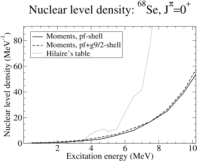
Figure 2: The same as Fig. 1 for ⁶⁸Se.

We illustrate the results by applications of the method to several nuclei important for astrophysics. Fig. 1 shows the level density for the $N=Z$ nucleus ⁶⁴Ge, states $J^{\pi}=0^{+}\;{\rm and}\;2^{+}$. Fig. 2 gives the same for ⁶⁸Se. In all four cases, the results for a larger orbital space, $pf+g_{9/2}$ shells, only slightly exceed those for the $pf$ space. However, as it is typical for all our calculations, the shell-model level density is very smooth as a function of energy and turns out to be much lower than what can be found from the tables [10]. The preliminary conclusion is that the full set of effective shell-model interactions responsible for emergence of quantum chaos is very important smoothing the results based mainly on the mean-field combinatorics.

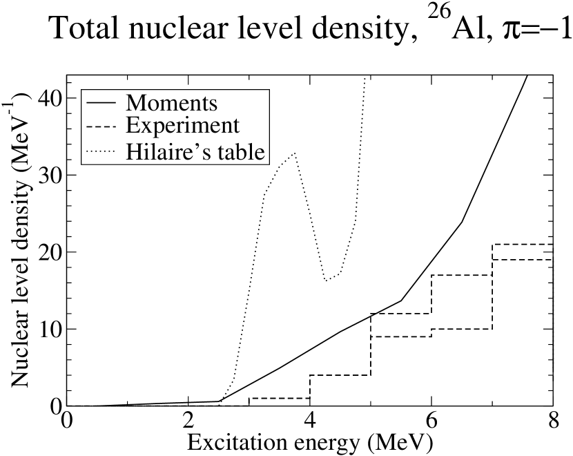
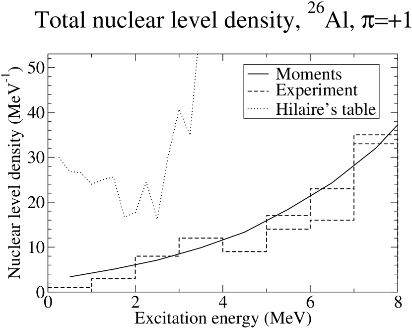
Figure 3: ²⁶Al, s-p-sd-fp-model space, all spins, WBT interaction [35]. Nuclear level densities are presented for negative (left figure) and positive (right figure) parities. Solid lines present the results of the Moments method, dashed lines show experimental level density (upper and lower lines correspond to experimental uncertainties in level identification), and dotted lines present the total level densities of Ref. [10].

In Fig. 3 we compare the total level density (for positive and negative parity separately) in ²⁶Al, calculated in the large s-p-sd-fp-model space restricted by $1\hbar\omega$ excitations only, with the WBT interaction [35]. For this isotope a good set of data is available and it is possible to juxtapose the results of our approach to those of the full shell-model diagonalization. Again, we obtain much lower and smoother level density than predicted by tables [10]. The two dashed stair-case lines show the data (“optimistic” and “pessimistic” estimates of uncertainties in identification of level parity). The calculations reasonably well describe available data.

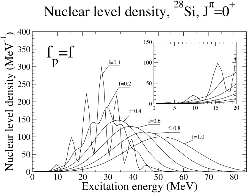
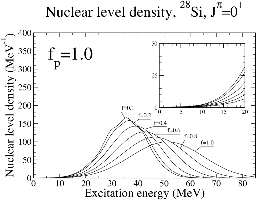
Figure 4: ²⁸Si, $J^{\pi}=0^{+}$, $sd$-model space, USDB interaction [36]. Different curves correspond to different scale factors $f$, see Eq. (6). Left panel presents the case when $f_{p}=f$, i.e. pairing and non-pairing parts of the interaction scales similarly. Right figure presents the case when pairing interaction is always on, $f_{p}=1$, while non-pairing interaction scales. The inset shows the low-energy part.

Using the Moments method we can study dependence of the level densities on the interaction. Let us scale the shell model two-body interaction with two factors, $f$ and $f_{p}$:

$$H=\epsilon+f_{p}V(\mbox{pairing})+fV(\mbox{non-pairing}),$$ (6)

where $\epsilon$ is the one-body part of the Hamiltonian, $V(\mbox{pairing})$ includes only the $J=0,T=1$ matrix elements of the two-body interaction, while $V(\mbox{non-pairing})$ includes all remaining matrix elements. Varying the scale factors $f$ and $f_{p}$ we can study the influence of different components of interaction onto the level density. Figs. 4 and 5 present examples of such an investigation for ²⁸Si level densities, calculated in the $sd$-model space, with the USDB interaction [36]. Fig. 4 presents results only for $J=0$ and Fig. 5 presents analogous calculations for all spins. Although dimensions and some details depend on $J$, the qualitative behavior is universal in all classes of states. The sharp irregularities related to the partition structure are rapidly smoothen even by the pairing interaction when it is accounted for exactly rather than in the BCS or HFB schemes. The remaining interactions broaden the level density and made its final tuning.

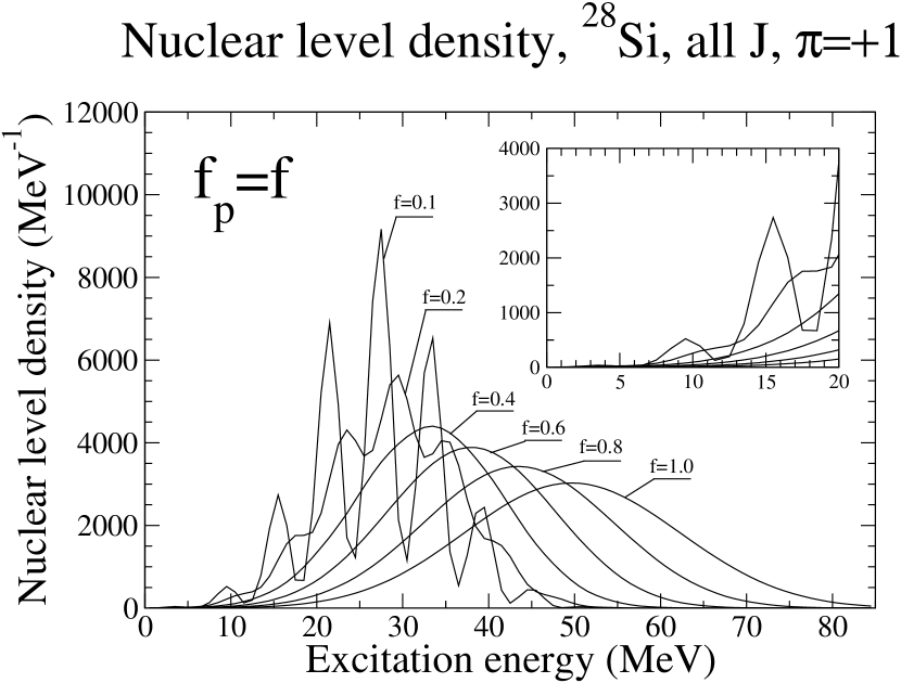
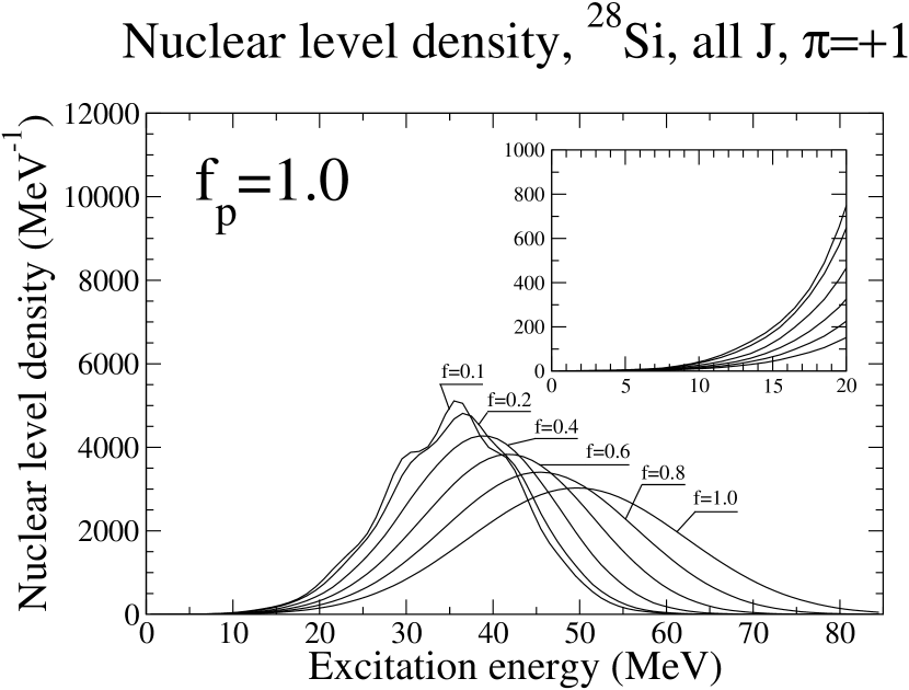
Figure 5: ²⁸Si, all $J$, $\pi=+1$, $sd$-model space. The description is similar to Fig. 4.

The natural next step in development of theory should be an attempt, in application to many nuclei, to extract the global empirical parameters, such as temperature, parameters of phenomenological fits, spin cut-off, and so on in order to bridge the gap between shell-model theory and convenient statistical descriptions used by experimentalists. Such studies also could help in selection of more reliable effective interactions for different regions of the periodic table. It might be that the global behavior of the level density is governed by few “coherent” interactions while the remaining abundant matrix elements are responsible for broadening and smoothing the stair-case behavior and can be modeled by an appropriately chosen “noise”. With parallelization of calculations [23], they can be extended to larger many-shell spaces. Finally, we have to confess that the problem of continuum effects is still waiting for its proper consideration.

References

References

- [1] Frenkel Ya I 1936 Sow. Phys. 9 533
- [2] Bethe H 1936 Phys. Rev. 50 332
- [3] Bethe H 1937 Rev. Mod. Phys. 9 69
- [4] Landau L D 1937 J. Exp. Theor. Phys. 7 819
- [5] Bohr N 1936 Nature 137 344
- [6] Ericson T 1960 Adv. Phys. 9 425
- [7] Gilbert A and Cameron A G W 1965 Can. J. Phys. 43 1446
- [8] Goriely S, Hilaire S, and Koning A J 2008 Phys. Rev. C 78 064307
- [9] Goriely S, Hilaire S, Koning A J, Sin M, and Capote R 2009 Phys. Rev. C 79 024612
- [10] http://www.astro.ulb.ac.be/pmwiki/Brusslib/Level
- [11] Alhassid Y, Liu S, and Nakada H 2007 Phys. Rev. Lett. 99 162504
- [12] Alhassid Y, Fang L, and Nakada H 2008 Phys. Rev. Lett. 101 082501
- [13] Teran E and Johnson C W 2006 Phys. Rev. C 73 024303; C 74 067302
- [14] Horoi M, Jora R, Zelevinsky V, Murphy A St J, Boyd R N, and Rauscher T 2002 Phys. Rev. C 66 015801
- [15] Horoi M, Kaiser J, and Zelevinsky V 2003 Phys. Rev. C 67 054309
- [16] Horoi M, Ghita M, and Zelevinsky V 2004 Phys. Rev. C 69, 041307(R)
- [17] Horoi M and Zelevinsky V 2007 Phys. Rev. Lett. 98 263503
- [18] Gao Z C and Horoi M 2009 Phys. Rev. C 79 014311
- [19] Gao Z C, Horoi M, and Chen Y S 2009 Phys. Rev. C 80 034325
- [20] Scott M and Horoi M 2010 EPL 91 52001
- [21] Sen’kov R A and Horoi M 2010 Phys. Rev. C 82 024304
- [22] Sen’kov R A, Horoi M, and Zelevinsky V 2011 Phys. Lett. B 702, 413
- [23] Sen’kov R A, Horoi M, and Zelevinsky V 2013 Comp. Phys. Comm. 184 215
- [24] Wong S S M 1986 Nuclear Statistical Spectroscopy (Oxford, University Press)
- [25] Kota V K B and Haq R U 2010 eds., Spectral Distributions in Nuclei and Statistical Spectroscopy (World Scientific, Singapore)
- [26] Zelevinsky V, Brown B A, Frazier N, and Horoi M 1996 Phys. Rep. 276 85
- [27] Jacquemin C 1981 Z. Phys. A 303 135
- [28] Van Isacker P 2002 Phys. Rev. Lett. 89 262502 (2002)
- [29] Pillet N, Zelevinsky V, Dupuis M, Berger J-F, and Daugas J M 2012 Phys. Rev. C 85 044315
- [30] Zelevinsky V and Volya A 2004 Phys. Rep. 391 311
- [31] Launey K D, Sarbadhicary S, Dytrych T and Draayer J P 2013, Comp. Phys. Comm. in press
- [32] Brody T A, Flores J, French J B, Mello P A, Pandey A, and Wong S S M 1981 Rev. Mod. Phys. 53 385
- [33] Horoi M, Volya A, and Zelevinsky V 1999 Phys. Rev. Lett. 82 2064
- [34] Horoi M, Brown B A, and Zelevinsky V 2002 Phys. Rev. C 65 027303
- [35] Warburton E K and Brown B A 1992 Phys. Rev. C 46 923
- [36] Brown B A and Wildenthal B H 1988 Annu. Rev. Nucl. Part. Sci. 38 29