High-order harmonic generation from Rydberg states at fixed Keldysh parameter

Abstract

Because the commonly adopted viewpoint that the Keldysh parameter $\gamma$ determines the dynamical regime in strong field physics has long been demonstrated to be misleading, one can ask what happens as relevant physical parameters, such as laser intensity and frequency, are varied while $\gamma$ is kept fixed. We present results from our one- and fully three-dimensional quantum simulations of high-order harmonic generation (HHG) from various bound states of hydrogen with $n$ up to 40, where the laser intensities and the frequencies are scaled from those for $n=1$ in order to maintain a fixed Keldysh parameter $\gamma$$<1$ for all $n$. We find that as we increase $n$ while keeping $\gamma$ fixed, the position of the cut-off scales in well defined manner. Moreover, a secondary plateau forms with a new cut-off, splitting the HHG plateau into two regions. First of these sub-plateaus is composed of lower harmonics, and has a higher yield than the second one. The latter extends up to the semiclassical $I_{p}+3.17U_{p}$ cut-off. We find that this structure is universal, and the HHG spectra look the same for all $n\gtrsim 10$ when plotted as a function of the scaled harmonic order. We investigate the $n$-, $l$- and momentum distributions to elucidate the physical mechanism leading to this universal structure.

I Introduction

High harmonic generation (HHG) is a nonlinear phenomenon in which atoms interacting with an intense laser pulse emit photons whose frequencies are integer multiples of the driving laser frequency. The emphatic motivation is the generation of spatially and temporally coherent bursts of attosecond pulses with high frequencies covering a range from vacuum ultraviolet (VUV) to the soft x-ray region hentschel . Filtering the high-frequency part of a high-harmonic spectrum allows the syntheses of ultrashort, coherent light pulses with energies in the extreme ultraviolet (XUV) part of the spectrum. This allows for tracing and controlling electronic processes in atoms, as well as coupled vibrational and electronic processes in molecules worner ; itatani . Some of the most visible applications of ultrashort pulses of attosecond duration involve resolving the electronic structure with high degree of spatial and temporal resolution chen , controlling the dynamics in the XUV-pumped excited molecules rini , and exciting and probing inner-shell electron dynamics with high resolution sandberg . Time-resolved holography tobey , imaging of molecular orbitals itatani , and attosecond streaking itatani2 are also among the state-of-the-art applications of HHG.

High-order harmonic generation is a process well described within the semi-classical three step model (ionization, propagation followed by recombination). The plateau region, where consecutive harmonics have approximately the same intensity, constitutes the main body of a high-harmonic spectrum. First step of the three step model is the tunneling of the electron through the Coulomb potential barrier suppressed by the laser field. The second step is laser-driven propagation of the free electron, and the third step is the rescattering of the electron with its parent ion. During this last step, the electron can recombine with its parent ion and liberate its excess energy as a short wavelength harmonic photon. The three step model predicts that the highest kinetic energy that an electron gains during its laser-driven excursion is given by $3.17U_{p}$, where $U_{p}=F^{2}/(4\omega_{0}^{2})$ is the quiver energy of the free electron in the laser field, and $F$ and $\omega_{0}$ are the laser field amplitude and frequency. The highest harmonic frequency, $\omega_{c}$, that can be generated within this model is $q_{\max}\omega_{0}=\left|{E_{b}}\right|+3.17U_{p}$, where $\left|{E_{b}}\right|$ is the binding energy of electron in the atom and $q_{\max}$ is the order of the cut-off harmonic corkum .

A crucial assumption in this physical picture is that the electron tunnels into the continuum in the first step in a laser field characterized by a small Keldysh parameter. This liberates the electron with no excess kinetic energy, and its subsequent excursion is driven by the classical laser field alone. Keldysh parameter $\gamma$ is commonly used to refer to one of the two dominant ionization dynamics in strong fields; tunneling or multiphoton regimes keldysh . It is defined as the the time it takes for the electron to tunnel the barrier in units of the laser period, i.e., $\gamma\sim\tau/T$. Here $\tau$ is the tunneling time and $T=2\pi/\omega_{0}$ is the laser period. If the tunneling time is much smaller than the laser period, one could expect that it is likely for the electron to tunnel through the barrier. In contrast, if tunneling time is much longer than the laser period, then the electron doesn’t have enough time tunnel through the depressed Coulomb barrier, and ionization can only occur through photon absorption. The Keldysh parameter can be expressed as $\gamma=\omega_{0}\sqrt{2\left|{E_{b}}\right|}/F$ keldysh .

Although the Keldysh parameter is widely used to refer to the underlying dynamics in strong field ionization, there are studies which suggest that it is an inadequate parameter in making this assessment reiss1 ; reiss2 ; topcu12 when a large range of laser frequencies are considered. Thus, it is natural to ask what happens in the strong field ionization step of HHG as a function of $n$, as relevant parameters, such as laser intensity and frequency, are varied while $\gamma$ is kept fixed. In this paper, we investigate the HHG process from the ground and the Rydberg states of a hydrogen atom using a one-dimensional $s$-wave model supported by fully three-dimensional quantum simulations. The central idea is that in a hydrogen atom, both the field strength $F$ and the frequency $\omega_{0}$ scale in a particular fashion with the principal quantum number $n$. Scaling the field strength by $1/n^{4}$ and the frequency by $1/n^{3}$, it is evident that $\gamma=\omega_{0}\sqrt{2\left|{E_{b}}\right|}/F$ remains unaffected as $n$ is changed, provided that both $F$ and $\omega_{0}$ are scaled accordingly while $n$ is varied.

In the spirit of the Keldysh theory, going beyond the ground state and starting from higher $n$ as the initial state, scaling $F$ and $\omega_{0}$ to maintain a fixed value of $\gamma$ should keep the ionization step of the harmonic generation in the same dynamical regime. We calculate HHG spectra starting from the ground state of hydrogen using laser parameters for which $\gamma<1$ (tunneling), and then calculate the high-harmonic spectra from increasingly larger $n$-states, scaling $F$ and $\omega_{0}$ from the ground state simulations and keep $\gamma$ fixed. If the Keldysh parameter is indeed adequate in referring to the ionization step properly in HHG, one should expect that the physics of the three-step process would remain unchanged, as the remainder of the steps involve only classical propagation of the electron in the continuum, and the final recombination step, which is governed by the conservation of energy.

There are a number of studies devoted to HHG from Rydberg atoms. The main motivation in these efforts are primarily increasing the conversion efficiency in the harmonic generation to obtain higher yields, which in turn would enable the generation of more intense attosecond pulses. Hu et al. hu demonstrated that, by stabilization of excited outer electron of the Rydberg atom in an intense field, a highly efficient harmonic spectrum could be generated from the more strongly bound inner electrons. In another recent study, Zhai et al. zhai1 ; zhai2 proposed that an enhanced harmonic spectrum is possible if the initial state is prepared as a superposition of the ground and the first excited state. The idea behind this method is that when coupled with the ground state, ionization can occur out of the excited state, initiating the harmonic generation. Since the excited state has lower ionization potential than the ground state, this in principle can result in higher conversion efficiency if the electron subsequently recombines into the excited state. In this scenario, the high-harmonic plateau would still cut-off at the semiclassical limit $I_{p}+3.17U_{p}$ with $I_{p}$ being that of the excited state. If, however, upon ionization out of the excited state, the electron recombines into the ground state, the cut-off can be pushed up to higher harmonics. Same principle is also at play in numerous studies proposing two-color driving schemes for HHG, with one frequency component serving to excite the ground state up to an excited level with a lower ionization potential, thus increasing the ionization yield (see for example zhai3 ).

In this paper, we report HHG spectra from ground and various Rydberg states with $n$ up to 40 for hydrogen atom, where the laser intensity and the frequency are such that the ionization step occurs predominantly in the tunneling regime. Starting with $\gamma=0.755$ at $n=1$, we go up in $n$ of the initial state and scale $F$ by $1/n^{4}$ and $\omega_{0}$ by $1/n^{3}$, keeping $\gamma$ constant. We discuss the underlying mechanism in terms of field ionization and final $n$-distributions after the laser pulse. We find that the harmonic order of the cut-off predicted by the semiclassical three-step model scales as $1/n$ when $F$ and $\omega_{0}$ are scaled as described above, and $\gamma$ is kept fixed. We repeat some of these model simulations by solving the fully three-dimensional time-dependent Schrödinger equation to investigate the effects which may arise due to angular momenta in high-$n$ manifolds. For select initial $n$ states, we look at momentum distributions of the ionized electrons, and the wave function extending beyond the peak of the depressed Coulomb potential at $1/\sqrt{F}$. Unless otherwise stated, we use atomic units throughout.

II One-dimensional calculations

The time-dependent Schrödinger equation of an electron interacting with the proton and the laser field $F(t)$ in the $s$-wave model in length gauge reads

$$\rm i\;\frac{\partial\psi(r,t)}{\partial t}=\left[-\frac{1}{2}\frac{{{d}^{2}}}{d{{r}^{2}}}-\frac{1}{r}+rF(t)\right]\psi(r,t).$$ (1)

In our simulations, time runs from $-t_{f}$ to $t_{f}$. This choice of time range centers the carrier envelope of the laser at $t=0$, which simplifies its mathematical expression. We choose the time-dependence of the electric field $F(t)$ to be

$$F(t)={F_{0}}\exp(-(4\ln 2){{t}^{2}}/{{\tau}^{2}})\cos({{\omega}_{0}}t),$$ (2)

where $F_{0}$ is the peak field strength, $\omega_{0}$ is the laser frequency and $\tau$ is the field duration at FWHM. Our one dimensional model is an $s$-wave model and restricted to the half space $r\geq 0$ with a hard wall at $r=0$. Having a hard wall at $r=0$ when there is no angular momentum can potentially be problematic, because the electron can absorb energy from the hard wall when using $-1/r$ potential. However, we believe that this model is adequate for the problem at hand, because we are deep in the tunneling regime. In our calculations, the number of photons required for ionization to occur through photon absroption is $\sim$9 for $n=1$, approaches to 71 by $n=10$ and stays so for higher $n$. As a result, ionization takes place primarily in the tunneling regime. If an extra photon is absorbed at the hard wall, its effect would mostly concern the lowest harmonics, which we are not interested in. In Sec. III, we show that the results we obtain in this section are consistent with our findings from fully three-dimensional calculations.

We consider cases in which the electron is initially prepared in an $ns$ state, where $n$ ranges from 1 up to 40. Our pulse duration is 4-cycles at FWHM for each case, and the wavelength of the laser field is 800 nm for the ground state. This gives a 2.7 fs optical cycle when the wavelength is 800 nm. Thus, the total pulse duration $\tau$ for the ground state is $\sim$11 fs and it scales as $n^{3}$. For the 4s state, this results in a pulse duration of $\sim$704 fs, while it amounts to $\sim$5.6 ps for the 8s state.

For the numerical solution of equation (1), we perform a series of calculations to make sure that the mesh and box size of the radial grid and the time step we use are fine enough so that our results are converged to within a few per cent. As we go beyond the 1s state, we increase the radial box size to accommodate the growing size of the initial state and the interaction region. We propagate Eq. (1) for excited states using a square-root mesh of the form ${{j}^{2}}\delta r$, where $j$ is the index of a radial grid point, $\delta r=R/{{N}^{2}}$, $R$ is the box size, and $N$ is the number of grid points. This type of grid is more efficient than using a uniform mesh in problems involving Rydberg states topcu07 , because it puts roughly the same number of points between the successive nodes of a Rydberg state. For the ground state, the box size is $R=750$ a.u. and ${N}=800$, which gives ${\delta r}=0.0012$ a.u.. For excited states, the box size grows $\sim{{n}^{2}}$ and with a proper selection of ${\delta r}$, we make sure that the dispersion relation $k\delta r=0.5$ holds for each $n$ state, where $k$ is the maximum electron momentum acquired from the laser field: $k=\sqrt{2{{E}_{\max}}}$ and ${{E}_{\max}}=3.17{{U}_{p}}$.

The time propagation of the wave-function is carried out using an implicit scheme. For the temporal grid spacing $\delta t$, we use $n^{3}$/180 of a Rydberg period, which is small enough to give converged results. A smooth mask function which varies from 1 to 0 starting from 2/3 of the way between the origin and the box boundary is multiplied with the solution of equation (1) at each time step to avoid spurious reflections from the box boundaries.

The time-dependent solutions of equation (1) are obtained for each initial $ns$ state, which we then use to calculate the time-dependent dipole acceleration, $a(t)=\langle\ddot{r}\rangle(t)$:

$$a(t) = \langle\psi(r,t)|\left[H,\left[H,r\right]\right]|\psi(r,t)\rangle\;.$$ (3)

Because the harmonic power spectrum is proportional to the Fourier transform of the squared dipole acceleration, we report $|a(\omega)|^{2}$ for harmonic spectra.

The initial wave function is normalized to unity, and the time-dependent ionization probability is calculated as the remaining norm inside the spatial box at a given time $t$,

$$P(t)=1-\int\limits_{0}^{{R}}{{{\left|\psi(r,t)\right|}^{2}}dr}.$$ (4)

In evaluation of the ionization probability, we propagate the wavefunction long enough after the pulse is turned off until $P(t)$ converges to a time-independent value.

II.1 Results and discussion

In our one-dimensional simulations, we consider cases where the atom is initially in an $n$s state with $n$ up to 40. The laser parameters are critically chosen so that the Keldysh parameter is fixed at $\gamma=0.755$ for each initial $n$, and the scaled frequency of the laser field is ${{\omega}_{0}}{{n}^{3}}\ll 1$, i.e., the electric field has a slowly varying time-dependence compared with the Kepler period ${{T}_{K}}=2\pi{n}^{3}$ of the Rydberg electron. For example, for an 800 nm laser, an optical cycle is $\sim$18 times the Kepler period for $n=1$. The cut-off frequency ${{\omega}_{c}}$ predicted by the three-step model is ${{\omega}_{c}}=\left|{{E}_{b}}\right|+3.17{{U}_{p}}$ corkum , where ${{U}_{p}}=F^{2}/4\omega_{0}^{2}$ is the ponderomotive potential. Since $\left|{{E}_{b}}\right|$, ${F}$ and ${{\omega}_{0}}$ scale as ${{n}^{-2}}$, ${{n}^{-4}}$ and ${{n}^{-3}}$ respectively, the cut-off frequency ${{\omega}_{c}}$ scales as ${{n}^{-2}}$ and the harmonic order of the cut-off ${{q}_{\max}}={{\omega}_{c}}/{{\omega}_{0}}$ scales as $n$ for fixed $\gamma$.

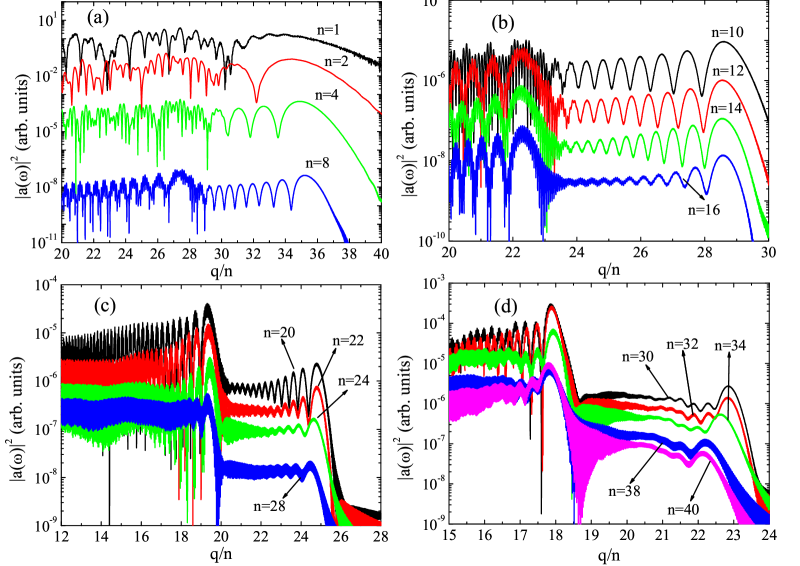
Figure 1: (Color online) High harmonic spectrum from the Rydberg states of H atom. The scaled laser field intensities and the wavelengths are, (a) 200/${{n}^{8}}$ TW/cm² and 800${{n}^{3}}$ nm, (b) 300/${{n}^{8}}$ TW/cm² and 652${{n}^{3}}$ nm, (c) 400/${{n}^{8}}$ TW/cm² and 566${{n}^{3}}$ nm, (d) 470/${{n}^{8}}$ TW/cm² and 522${{n}^{3}}$ nm. The width of the laser pulse is 4-cycles at FWHM, and the selected parameters correspond to $\gamma=0.755$ in each case. The scaled harmonic order is $q/n$, where $q=\omega/{{\omega}_{0}}$ is the harmonic order.

Harmonic spectra from these simulations are seen in Fig. 1 (a)-(d) as a function of the scaled harmonic order $\widetilde{q}=q/n$, where $q=\omega/\omega_{0}$ is the harmonic order. In Fig. 1 (a), the scaled laser intensity and the wavelength are $200/{{n}^{8}}$ TW/cm² and 800${{n}^{3}}$ nm, which correspond to $\gamma=0.755$. The most prominent feature in these spectra is a clear double plateau structure, exhibiting one plateau with a higher yield and another following with lower yield. The second plateau terminates at the usual semiclassical cut-off. These plateaus are connected with a secondary cut-off, which converges to a fixed scaled harmonic order $\widetilde{q}=q/n$ as $n$ becomes large.

We also note that the overall size of $|a(\omega)|^{2}$ drops significantly with increasing $n$ in Fig. 1 (a). For example, going from $n=2$ to $n=4$, $|a(\omega)|^{2}$ drops about 3 orders of magnitude, and from $n=4$ to $n=8$ it drops roughly 4 orders of magnitude. The spectrum obtained for $n=8$ is about 9 orders of magnitude lower than that for $n=1$. Beyond $n=8$, the overall sizes of the spectra are too small and plagued by numerical errors, which is why we stop at $n=8$ in panel (a). This is because the amplitude of the wave function component contributing to the three-step process is too small to yield a meaningful spectrum within our numerical precision. In order to ensure sizable HHG spectra while climbing up higher in $n$, we adopt the following procedure: We split the Rydberg series into different groups of initial $n$-states, which are subject to different laser parameters but have the same $\gamma$ value within themselves. Within each group, we climb up in $n$ by scaling the laser parameters for the lowest $n$ in the group until $|a(\omega)|^{2}$ becomes too small. We then move onto the next group of $n$-states, increasing the laser intensity and the frequency ($\gamma\propto\omega/F$) for the lowest $n$ in the group while attaining the same $\gamma$ as in the previous $n$-groups. Scaling this intensity and frequency, we continue to climb up in $n$ until again $|a(\omega)|^{2}$ becomes too small, at which point we terminate the group and move onto the next.

Following this procedure, we are able to achieve HHG spectra for states up to $n=40$ in Fig. 1. The first $n$-group in panel (a) includes states between $n=1-8$, and the laser intensity and wavelength are $200/{{n}^{8}}$ TW/cm² and 800${{n}^{3}}$ nm. In panel (b) is the second group with $n=10-18$ and the laser parameters $300/{{n}^{8}}$ TW/cm² and 652${{n}^{3}}$ nm. In panel (c), $n=20-28$ and the laser parameters are $400/{{n}^{8}}$ TW/cm² and 566${{n}^{3}}$ nm, and finally in panel (d), $n=30-40$ with intensity and wavelength $470/{{n}^{8}}$ TW/cm² and 522${{n}^{3}}$ nm. The peak field strengths corresponding to these intensities are lower than the critical field strengths for above-the-barrier ionization for the states we consider, and the ionization predominantly takes place in the tunneling regime.

The dipole accelerations at the two cut-off harmonics for each $n$-group seen in Fig. 1 (a)-(d) are plotted in the upper two panels of Fig. 2. Here, we plot $|a(\omega)|^{2}$ as a function of $n$. This figure points to a situation in which $|a(\omega)|^{2}$ drops with increasing $n$ within each group of $n$. Also, for the first few $n$-groups, $|a(\omega)|^{2}$ drops much faster compared to those involving higher $n$. The reason for the decreasing $|a(\omega)|^{2}$ within each $n$-group in Fig. 2, can be understood by calculating the ionization probabilities in each case, and examining how it changes as $n$ is varied.

Although completely ionized electrons do not contribute to the HHG process, ionization and HHG are two competing processes in the tunneling regime. As a result, decrease in one alludes to decrease in the other. The ionization probabilities from the $n$s states in Fig. 1 are plotted against their principal quantum numbers in the lowest panel of Fig. 2. It is clear that as we go beyond the ground state, the ionization probabilities drop significantly as $n$ is increased within each group. This decrease is rather sharp for the first group and it levels off as we go to successive groups involving higher $n$. The values of the scaled frequencies $\Omega={\omega}{n}^{3}$ are the same in each $n$-group, and the laser parameters are chosen so as to make sure the condition $\Omega\ll 1$ holds. This ensures that the ionization is not hindered by processes such as dynamic localization. The reason behind the decreasing ionization probabilities within each $n$-group can be understood using the quasiclassical formula keldysh for the tunneling ionization rate:

$${{\Gamma}_{K}}\propto{{\left(\left|{{E}_{b}}\right|{{F}^{2}}\right)}^{1/4}}\exp\left(-2{{(2\left|{{E}_{b}}\right|)}^{3/2}}/3F\right)\;.$$ (5)

The laser field intensity and electron binding energy scale as $\sim$$1/{{n}^{4}}$ and $\sim$$1/{{n}^{2}}$. Thus, the exponent in the exponential factor in $\Gamma_{K}$ scales as $1/n$, which results in decreasing ionization probabilities within each $n$-group when plotted as a function of $n$ in the lowest panel of Fig. 2. This behavior is reflected in the corresponding HHG spectra in Fig. 1 and the upper panels in Fig. 2 as diminishing of the HHG yield.

The decrease in the ionization probability also slows down as as we successively move onto groups of higher $n$, as indicated by the decreasing slopes of the ionization probabilities in Fig. 2 between successive $n$-groups. We find that the ratio of the ionization probabilities between the 2s and 4s states in Fig. 2 is $\sim$39, whereas between the 12s and 14s states it is $\sim$7, between 22s and 24s states $\sim$3, and between 32s and 34s states $\sim$2. This is an artifact of the scheme we employ in which we divide up the Rydberg series into successive groups of $n$s states to ensure sizable HHG spectra. The rate of decrease in the ionization probability in each group is determined by the slope of $\Gamma_{K}$, i.e., ${\rm d}\Gamma_{K}/{\rm d}n$. This slope is proportional to the laser intensity we pick for the lowest $n$ in each group in order to initiate it, and we scale it down by $1/n^{8}$ inside the group to keep $\gamma$ fixed. However, although this start-up intensity for each group is larger than what it would have been of we were to continue up in $n$ in the previous group, it is still smaller than the initial intensity in the previous group. This results in a decreased slope going through successive $n$-groups. Hence the decay rates for the ionization probability in successive groups taper off, which is reflected in the two upper panels in Fi.g 2.

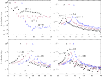
Figure 3: (Color online) The probability distributions in $n$ following the laser pulse for the initial states seen in Fig. 1. It is clear that the atom essentially resides in its initial state after the pulse, which means the recombination step in the harmonic generation process occurs primarily back to the initial state. The probability to find the atom in other nearby states is orders of magnitude smaller, and the probability distribution becomes symmetrical about the initial state for $n>10$ due to decreasing anharmonicity in the surrounding energy level structure.

We also calculate the final $n$-distributions for the atom after the laser pulse to see the extent of $n$ mixing which may have occurred during its evolution in the laser field. This is done by allowing the wave functions to evolve according to Eq. (1) long enough after the laser pulse to attain a steady state. We then project them onto the bound eigenstates of the atom to determine the final probability distributions $P(n)$ to find the atom in a given bound state. The results are shown in Fig. 3. It is evident from the figure that most of the wavefunction resides in the initial state after the laser pulse, and that there is small amount of mixing into adjacent $n$ states. The mixing is small because only a small fraction of the total wavefunction takes part in the HHG process. However, we cannot deduce from our calculations what fraction of the wavefunction actually participates in HHG, and hence what fraction of it spreads to higher $n$. Because the HHG and ionization are competing processes in this regime, the ionization probabilities seen in the bottom panel of Fig. 2 can be taken to be an indication of the amplitude that goes into the HHG process. For example, at $n=4$, the ionization probability is at $\sim$10% level in Fig. 2 and the largest amplitude after the laser pulse is in $n=5$ in Fig. 3 at 10^-5 level. This indicates that roughly a part in $10^{6}$ of the amplitude participating in the HHG process recombines into higher $n$-states. On the other hand, at $n=20$, the ionization probability is also at $\sim$10% level, but the spreading in $n$ is between $\sim$1% and $\sim$0.1% level, suggesting that between roughly 1 and 10% of the wavefunction participating the HHG process gets spread over adjacent $n$. In the recombination step of the HHG process, the probability for recombination back into the initial state is the largest, chiefly because the electron leaves the atom through tunneling with no excess kinetic kinetic energy. It largely retains the character of the initial state because its subsequent excursion in the laser field is classical and mainly serves for the electron wavepacket to acquire kinetic energy before recombination. In the next section, we discuss how this small spread helps shape the double plateau structure seen in Fig. 1.

III Three-dimensional Calculations

Three dimensional quantum calculations were carried out by solving the time-dependent Schrödinger equation as described in Ref. topcu07 . For sake of completeness, we briefly outline the theoretical approach below. We decompose the time-dependent wave function in spherical harmonics $Y_{\ell,m}(\theta,\phi)$ as

$$\Psi(\vec{r},t)=\sum_{\ell}f_{\ell}(r,t)Y_{\ell,m}(\theta,\phi)$$ (6)

such that the time-dependence is captured in the coefficient $f_{\ell}(r,t)$. For each angular momenta, $f_{\ell}(r,t)$ is radially represented on a square-root mesh, which becomes a constant-phase mesh at large distances. This is ideal for description of Rydberg states on a radial grid since it places roughly the same number of radial points between the nodes of high-$n$ states. On a square-root mesh, with a radial extent $R$ over $N$ points, the radial coordinate of points are $r_{j}=j^{2}\delta r$, where $\delta r=R/N^{2}$. We regularly perform convergence checks on the number of angular momenta we need to include in our calculations as we change relevant physical parameters, such as the laser intensity. For example, $\delta r=4\times 10^{-4}$ a.u. in a $R=2000$ a.u. box gave us converged results for $n=4$, whereas $\delta r=8\times 10^{-4}$ a.u. in a $R=2800$ a.u. box was sufficient at $n=8$. We also found that the number of angular momenta we needed to converge the harmonic spectra was much larger than $n-1$ for an initial $n$ state (e.g., $\sim$120 for the $n=8$ state).

We split the total hamiltonian into an atomic hamiltonian plus the interaction hamiltonian, such that $H(r,l,t)=H_{\text{A}}(r,l)+H_{\text{L}}(r,t)-E_{\text{0}}$. Note that we subtract the energy of the initial state from the total hamiltonian to reduce the phase errors that accumulate over time. The atomic hamiltonian $H_{\text{A}}$ and the hamiltonian describing the interaction of the atom with the laser field in the length gauge are

$$H_{\text{A}}(r,l) = -\frac{1}{2}\frac{\text{d}^{2}}{\text{d}r^{2}}-\frac{1}{r}+\frac{l(l+1)}{2r^{2}}\;,$$ (7)

$$H_{\text{L}}(r,t) = F(t)z\cos(\omega t)\;.$$ (8)

Contribution of each of these pieces to the time-evolution of the wave function is accounted through the lowest order split operator technique. In this technique, each split piece is propagated using an implicit scheme of order $\delta t^{3}$. A detailed account of the implicit method and the split operator technique employed is given in Ref. topcu07 . The interaction Hamiltonian, $F(t)r\cos(\theta)$, couples $\ell$ to $\ell\pm 1$. The laser pulse envelope has the same time-dependence as in the one-dimensional $s$-wave model calculations (Eq. 2).

The harmonic spectrum is usually described as the squared Fourier transform of the expectation value of the dipole moment ($d_{z}(t)=\langle z\rangle(t)$), dipole velocity ($v_{z}(t)=\langle\dot{z}\rangle(t)$), or the dipole acceleration ($a_{z}(t)=\langle\ddot{z}\rangle(t)$) (see bandrauk and references therein). In our three-dimensional calculations, we evaluate all three forms and compare them for different initial $n$ states:

$$d_{z}(t) = \langle\Psi(\vec{r},t)|z|\Psi(\vec{r},t)\rangle$$ (9)

$$v_{z}(t) = \langle\Psi(\vec{r},t)|\dot{z}|\Psi(\vec{r},t)\rangle$$ (10)

$$a_{z}(t) = \langle\Psi(\vec{r},t)|\ddot{z}|\Psi(\vec{r},t)\rangle\;,$$ (11)

where $\dot{z}=-\rm i[H,z]$ and $\ddot{z}=-[H,[H,z]]$. Ref. bandrauk found that the Fourier transforms $d_{z}(\omega)$, $v_{z}(\omega)$, and $a_{z}(\omega)$ are in good agreement when the pulses are long and “weak” in harmonic generation from the ground state of H atom, where “weak” refers to intensities below over-the-barrier ionization limit. As we increase the initial $n$ in our simulations keeping the Keldysh parameter $\gamma$ constant, we find that the agreement between these three forms of harmonic spectra gets better. This observation is in agreement with the findings in Ref. bandrauk , because to keep $\gamma$ fixed, we scale the pulse duration by $\sim$$n^{3}$ and the peak laser field strength by $\sim$$1/n^{4}$. Although the energy of the initial state is also scaled by $\sim$$1/n^{2}$ and the pulse duration is the same in number of optical cycles, the ionization probability drops within a given $n$-series in Fig. 2. This suggests that the pulse is effectively getting weaker as we increase $n$ for fixed $\gamma$. We report only the dipole acceleration form $|a_{z}(\omega)|^{2}$ to refer to harmonic spectra, chiefly because it is this form that is directly proportional to the emitted power, i.e., $S(\omega)=2\omega^{4}|a_{z}(\omega)|^{2}/(3\pi c^{3})$.

Because high-harmonic generation and ionization are competing processes in the physical regime we are interested in, it is useful to investigate the momentum distribution of the ionized part of the wave function to gain further insight into the HHG process. In order to evaluate the momentum distributions, we follow the same procedure outlined in Ref. vrakking . For sake of completeness, we briefly describe the method: In all simulations, the ionized part of the wave function is removed from the box every time step during the time propagation, in order to prevent unphysical reflections from the radial box edge. This is done by multiplying the wavefunction by a mask function $m(r)$ at every time step, where $m(r)$ spans 1/3 of the radial box at the box edge. We retrieve the removed part of the wave function by evaluating

$$\Delta\psi_{l}(r,t^{\prime})=[1-m(r)]\;\psi_{l}(r,t^{\prime})$$ (12)

at every time step, and Fourier transform it to get the momentum space wave function $\Delta\phi(p_{\rho},p_{z},t^{\prime})$,

$$\Delta\phi(p_{\rho},p_{z},t^{\prime})=2\; \sum_{l}(-i)^{l}\;Y_{l,m}(\theta,\varphi)$$

$$\times\int_{0}^{\infty}j_{l}(pr)\Delta\psi_{l}(r,t^{\prime})r^{2}\;dr\;.$$ (13)

Here the momentum $p=(p_{\rho}^{2}+p_{z}^{2})^{1/2}$ is in cylindrical coordinates and $j_{l}(pr)$ are the spherical Bessel functions. We then time propagate $\Delta\phi(p_{\rho},p_{z},t^{\prime})$ to a later final time $t$ using the semi-classical propagator,

$$\Delta\phi(p_{\rho},p_{z},t)=\Delta\phi(p_{\rho},p_{z},t^{\prime})\;e^{-iS}$$ (14)

where $S$ is the classical action. For the time-dependent laser field $F(t)$, action $S$ is calculated numerically by integrating $p_{z}^{2}$ along the laser polarization,

$$S = \frac{1}{2}p_{\rho}^{2}(t-t^{\prime})+\frac{1}{2}\int_{t^{\prime}}^{t}p_{z}^{2}dt^{\prime\prime}$$ (15)

$$p_{z} = \int_{t^{\prime}}^{t}F(t^{\prime\prime})dt^{\prime\prime}$$ (16)

We are assuming that the ionized electron is freely propagating in the classical laser field in the absence of the Coulomb field of its parent ion, and this method is numerically exact under this assumption.

III.1 Results and discussion

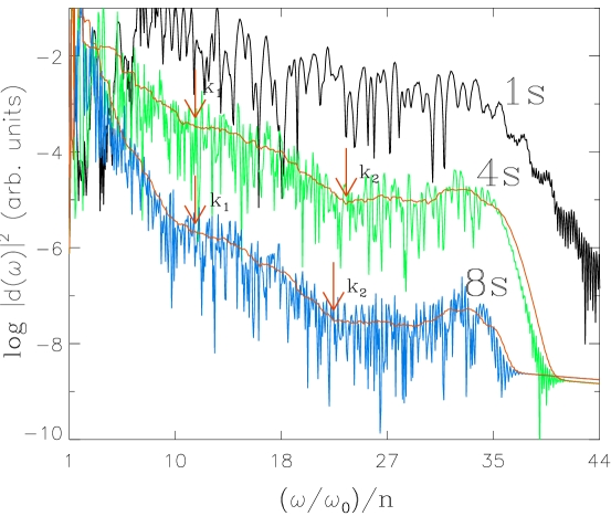
Figure 4: (Color online) Dipole acceleration from direct solution of the three-dimensional time-dependent Schrödinger equation when the atom is initially prepared in 1s, 4s and 8s states of H atom. The horizontal axis is the scaled harmonic order $\widetilde{q}\equiv q/n=(\omega/\omega_{0})/n$. There are three universal cut-off points in the spectra: marked as $k_{1}$, $k_{2}$, and the usual $I_{p}+3.17U_{p}$ limit. The double plateau structure mirrors that of the one-dimensional spectra from Fig. 1, with a universal secondary cut-off at $\widetilde{q}=23.45$. The arrows marked as $k_{1}$ and $k_{2}$ are discussed in the context of Fig. 7.

The double plateau structure we see in the one-dimensional spectra in Fig. 1 can be also observed from our three-dimensional simulations. In Fig. 4, the squared dipole acceleration $|a(\omega)|^{2}$ is plotted for the initial states of 1s (black), 4s (green), and 8s (blue) of Hydrogen atom as a function of the scaled harmonic order $\omega/(\omega_{0}n)\equiv\widetilde{q}$. In these calculations, we adhere to $\gamma=0.75$ as in the one-dimensional calculations, and start at $n=1$ with intensity $2\times 10^{14}$ W/cm² and $\lambda=800$ nm. From this, we use the $n$ scaling discussed in Sec. II.1 to determine the laser parameters for higher $n$ states. Apart from the double plateau structure, there is decrease in the HHG yield with increasing $n$ in Fig. 4, similar to the one-dimensional case. Again, this suggests that although $\gamma$ is fixed for all three initial states in Fig. 4, the atom sinks deeper into the tunneling regime as $n$ is increased, similar to what we have seen in the one-dimensional case in Sec. II.1. The main difference in Fig. 4 is that the first plateau is not as flat as in the one-dimensional calculations, as often the case when comparing one- and three-dimensional HHG spectra.

In order to clearly identify the first and the second cut-offs seen in Fig. 1, we have smoothened the 4s and 8s spectra by boxcar averaging to reveal their main structure (solid red curves) in Fig. 4. The usual scaled cut-off from the semiclassical three-step model is at $q_{\rm max}/n\simeq 35$ in all three spectra, and it is independent of $n$. A secondary cut-off emerges at the same scaled harmonic as in the one-dimensional case, which is labeled as $k_{2}$ in the 4s and the 8s spectra at $\widetilde{q}\simeq 23.45$. It is clear from Fig. 4 that just as the usual cut-off at $q_{\rm max}/n$, $k_{2}$ is also universal beyond $n>4$. This secondary cut-off separates the two plateaus, first spanning lower frequencies below $k_{2}$, and the second spanning higher frequencies between $k_{2}$ and $q_{\rm max}/n$.

The mechanism behind the formation of the secondary cut-off $k_{2}$ can be understood in terms of the ionization and the recombination steps of the semiclassical model. In the first step, the electron tunnels out of the initial $n$s state into the continuum, and has initially no kinetic energy. After excursion in the laser field, it recombines with its parent ion. In this last step, recombination occurs primarily back into the initial state. This is because the electron was liberated into the continuum with virtually no excess kinetic energy, and the electron wavepacket mainly retains its original character. When it returns to its parent ion to recombine, the recombination probability is highest for the bound state with which it overlaps the most. As a result, recombination into the same initial state is favored. This mechanism is associated with the usual cut-off since its position depends on the ionization potential: $q_{\rm max}=(I_{p}+3.17U_{p})/\omega_{0}$.

On the other hand, there is still probability that the electron can recombine to higher $n$ states. This would result in lower harmonics because less than $I_{p}$ needs to be converted to harmonics upon recombination. The cut-off for this mechanism would be achieved when the electron recombines with zero energy near the threshold ($n\rightarrow\infty$). Because the maximum kinetic energy a free electron can accumulate in the laser field is $3.17U_{p}$, the lower harmonic plateau would cut off at $3.17U_{p}$. For the laser parameters used in Fig. 4, this corresponds to the scaled harmonic $\widetilde{q}=23.45$, which is marked by the red arrows labeled as $k_{2}$ on the 4s and the 8s spectra. To reiterate, the second plateau with higher harmonics includes:

1. trajectories which recombine to the initial state ($n_{1}\rightarrow n_{1}$) after accumulating kinetic energy up to $3.17U_{p}$,

2. trajectories which recombine to a higher but nearby $n$ state ($n_{1}\rightarrow n_{2}$, where $n_{2}>n_{1}$) that have acquired kinetic energy up to $3.17U_{p}$,

3. trajectories which recombine to much higher $n$ states ($n_{1}\rightarrow n_{2}$, where $n_{2}\gg n_{1}$) resulting in the cut-off at $\widetilde{q}=23.45$.

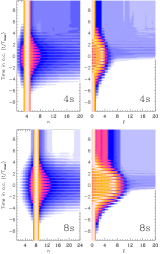
Figure 5: (Color online) $n$- and $l$-distributions for the probability to find the atom in 4s and 8s states of H for the laser parameters used in Fig. 4. All probabilities are plotted in $\log_{2}$ scale and the lowest contour in the $n$-distributions for both states is at the 10^-10 level. The half-cycles of the 4-cycle laser pulse are clearly visible.

The $n$- and $l$-distributions for the 4s and 8s states as a function of time can be seen in Fig. 5. Notice that the laser pulse is centered at $t=0$ o.c. and has 4 cycles at FWHM for both states. It is clear from the first column that the the atom mostly stays in the initial state and only a small fraction of the wavefunction contributes to the HHG process. To appreciate how small, we note that the highest contour is at unity, and lowest contour for both the 4s and the 8s states are at the $\sim$10^-10 level. At the end of the pulse, there is a small spread in $n$, which is skewed towards higher $n$ in both cases. This skew is expected since the energy separation between the adjacent $n$ manifolds drop as $\sim$$1/n^{3}$, and therefore it is easier to spread to the higher $n$ manifolds than to lower $n$. The small amplitude for this spread is a consequence of the fact that we are not in the $n$-mixing regime. In the second column, we see that the orbital angular momentum $l$ also spreads to higher $l$ within the initial $n$-manifold, and the small leakage to higher angular momenta at the end of the pulse is a consequence of the small probability for spreading to the higher $n$-manifolds.

The second step of the harmonic generation process involving the free evolution of the electron in the laser field be understood on purely classical grounds. It was the classical arguments that led to the $3.17U_{p}$ limit for the maximum kinetic energy attainable by a free electron. In the context of this paper, performing such classical simulations can yield no insight to how the excursion step of the HHG behaves under the scaling scheme we have employed so far. This is because the classical equations of motion perfectly scale under the transformations $r\rightarrow rn^{2}$, $t\rightarrow tn^{3}$, $\omega\rightarrow\omega/n^{3}$, and $E\rightarrow E/n^{2}$, where $r$ is distance and $t$ is time. On the other hand, it is the lack of this perfect scaling property of the Schrödinger equation that accounts for the differences between different initial $n$ states we have seen from our quantum simulations. One way to examine the excursion step by itself in our quantum simulations is to look at the momentum distribution of the part of the wavefunction that contributes to the HHG spectra.

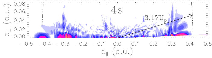
Figure 6: The momentum distribution for the ionized part of the wave function integrated over time until after the laser pulse when the atom is initially prepared in the 4s state. The total momentum $\sqrt{p^{2}_{||}+p^{2}_{\perp}}$ corresponding to the maximum kinetic energy that can be attained by a free electron in a laser field is marked by the dot-dashed semicircle and labeled as $3.17U_{p}$. This is the limit that determines the semiclassical cut-off at $q_{\rm max}=I_{p}+3.17U_{p}$.

To this end, we calculate the momentum map of the ionized part of the wavefunction when the atom is initially prepared in the 4s state. The reason we look at the ionized part of the wavefunction is because harmonic generation and ionization are competing processes. Therefore one would expect that they should mirror each other in their behavior. Fig. 6 shows this momentum distribution obtained by Fourier transforming the ionized part of the wavefunction, which is accumulated over time until after the laser pulse (see Eq. (12) onward). Since the problem has cylindrical symmetry, the horizontal axis is labeled $p_{||}$ to refer to the momentum component parallel to the laser polarization direction (same as $p_{z}$). The vertical axis $p_{\perp}$ is the perpendicular component. We have also labeled the $3.17U_{p}$ limit for the maximum kinetic attainable, which is along the dot-dashed semicircle. As expected, the total momentum of the escaped electrons cut off at $3.17U_{p}$, and the components which would have contributed to the two different plateaus in Fig. 4 are visible close to the laser polarization direction.

We also look at the momentum map of the wavefunction inside our numerical box that falls beyond the peak of the depressed Coulomb potential at $r=1/\sqrt{F}$. Part of the wavefunction in the region $r<1/\sqrt{F}$ is removed by multiplying it with a smooth mask function before the Fourier transformation step described in Sec. III. The results when the atom is initially in the 4s and 8s states are seen in Fig. 7 at five instances during the laser cycle at the peak of the pulse (labeled A, B, C, D, and E). We have also labeled three semicircles corresponding to three momenta $\sqrt{p^{2}_{||}+p^{2}_{\perp}}$ of interest:

1. the $3.17U_{p}$ limit, also seen in Fig. 6,

2. $k_{1}$ corresponding to the kinetic energy $U_{p}$,

3. $k_{2}$ corresponding to the kinetic energy necessary to emit the harmonic $\widetilde{q}=23.45$ at the secondary cut-off in Fig. 4, if the electron recombines into its initial 4s or 8s state upon rescattering.

The amplitude inside the $k_{1}$ semicircle contributes to only very low harmonics, below the scaled harmonic labeled as $k_{1}$ in Fig. 4. This part of the spectra is not suitable for the semiclassical three step description of HHG. The annular region between the semicircles $k_{1}$ and the $k_{2}$ contributes to the first low harmonic plateau in Fig. 4. Finally, the region between $k_{2}$ and the semiclassical $3.17U_{p}$ limit contributes to the less intense second plateau. The distinction between the lower harmonics from the inner $k_{1}$ semicircle and the higher harmonics from the annular region between $k_{1}$ and $k_{2}$ is manifested most clearly in the 4s column, as longer and shorter wavelengths in the momentum maps inside these regions. Expectedly, both momentum maps for the 4s and the 8s initial states show the same structures, the essential difference being the number of nodes in the momentum space wave functions which scales as $n^{2}$. Incidentally, a rescattering event is visible on the laser polarization axis at $k_{2}$ in panel D of the 4s column, giving rise to kinetic energy beyond the $3.17U_{p}$ limit on the left.

IV Conclusions

We have presented results from one- and three-dimensional time-dependent quantum calculations for higher-order harmonic generation from excited states of H atom for a fixed Keldysh parameter $\gamma$. Starting from the ground state, we chose laser intensity and frequency such that we are in the tunneling regime and ionization probability is well below one per cent. We then scale the intensity by $1/n^{8}$ and the frequency by $1/n^{3}$ to keep $\gamma$ fixed as we increase the principal quantum number $n$ of the initial state of the atom. Because $\gamma$ is fixed, the common wisdom is that the dynamical regime which determine the essential physics should stay unchanged in the HHG process as we go up in $n$ of the initial state. Our one-dimensional calculations demonstrate that this is indeed the case, and although the emitted power (HHG yield) drops as we climb up in $n$, the resulting harmonic spectra display same universal features beyond $n$$\sim$10. The most distinguished feature that develops when the atom is initially prepared in a Rydberg state is the emergence of a secondary plateau below the semiclassical cut-off $q_{\rm max}$ in the HHG plateau. This secondary cut-off splits the harmonic plateau into two regions: one spanning low harmonics and terminating with a secondary cut-off, and a second plateau with lower yield and higher harmonics terminating at the usual semiclassical cut-off at $q_{\rm max}$.

We have also found that the positions of these cut-off harmonics also scale as $1/n$, and introduced the concept of “scaled harmonic order”, $\widetilde{q}=\omega/(\omega_{0}n)$. When plotted as a function of $\widetilde{q}$, the harmonic spectra appear universal and, except for the overall yields, the spectra for high $n$ look essentially identical.

We then carried out fully three-dimensional calculations for three of the $n$ states in the lowest $n$-group in the one-dimensional calculations to gain further insight into the scaling properties we have seen in the one-dimensional calculations. This also serves to investigate possible effects of having angular momentum. We found the same features as in the one-dimensional spectra, except that the yield from the first plateau is skewed towards lower harmonics. We associate this with spreading to higher $n$ states during the tunnel ionization and recombination steps by analyzing the $n$- and $l$-distributions of the atom after the laser pulse. Momentum distributions of the ionized electrons and the wave function beyond the peak of the depressed Coulomb potential at $r=1/\sqrt{F}$ show features which we can relate to the universal features we see in the HHG spectra at high $n$. We identify the first plateau in this universal HHG spectrum with features in momentum space between two values of momentum: (1) the momentum corresponding to kinetic energy $U_{p}$, and (2) the momentum corresponding to kinetic energy if the electron emits the secondary cut-off harmonic upon recombining to its initial state. The latter case also occurs when the electron recombines to a much higher Rydberg state than the one it tunnels out after accumulating maximum possible kinetic energy of $3.17U_{p}$ during its excursion in the laser field.

V Acknowledgments

IY, EAB and ZA was supported by BAPKO of Marmara University. ZA would like to thank to the National Energy Research Scientific Computing Center (NERSC) in Oakland, CA. TT was supported by the Office of Basic Energy Sciences, US Department of Energy, and by the National Science Foundation Grant No. PHY-1212482.

Fig. 01

Fig. 02

$\begin{array}[]{c}\leavevmode\resizebox{284.52756pt}{}{\includegraphics{./fig_02a.pdf}}\\ \leavevmode\resizebox{293.06339pt}{}{\includegraphics{./fig_02b.pdf}}\end{array}$

Figure 2: (Color online) (Upper two panels) $|a(\omega)|^{2}$ at the 1st and 2nd cut-offs of the H atom as a function of $n$, obtained from Fig 1 (a)-(d). Within each $n$-group, the $|a(\omega)|^{2}$ drops with increasing $n$. (Lower panel) Ionization probabilities of H atom as a function of $n$ mimic the behavior of $|a(\omega)|^{2}$ in the upper panels. The field parameters are the same as in Fig. 1 (a)-(d).

Fig. 03

Fig. 04

Fig. 05

Fig. 06

Fig. 07

$\begin{array}[]{cc}\leavevmode\resizebox{210.55038pt}{}{\includegraphics{./fig_07a.pdf}}&\leavevmode\resizebox{239.00314pt}{}{\includegraphics{./fig_07b.pdf}}\end{array}$

Figure 7: (Color Online) Momentum distributions in the region $r>1/\sqrt{F}$ for the 4s (left column) and 8s (right column) states at five instances during the laser cycle at the peak of the pulse (indicated on top). The region $r>1/\sqrt{F}$ is beyond the peak of the Coulomb potential depressed by the strong laser field.

References

- (1) Hentschel M, Kienberger R, Spielmann Ch, Reider G A, Milosevic N, Brabec T, Corkum P B, Heinzmann U, M. Drescher and F. Krausz 2001 Nature 414 509.
- (2) Wörner H J, Bertrand J B, Kartashov D V, Corkum P B and Villeneuve D M 2010 Nature 466 604.
- (3) Itatani J, Levesque J, Zeidler D, Niikura H, Pepin H, Kieffer J C, Corkum P B and Villeneuve D M 2004 Nature 432 867.
- (4) Chen M -C , Arpin P, Popmintchev T, Gerrity M, Zhang B, Seaberg M, Popmintchev D, Murnane M M and Kapteyn H C 2010 Phys. Rev. Lett. 105 173901.
- (5) Rini M, Tobey R, Dean N, Itatani J, Tomioka Y, Tokura Y, Schoenlein R W and Cavalleri A 2007 Nature 449 6.
- (6) Sandberg R L et al. 2009 Opt. Lett. 34 1618.
- (7) Tobey R I, Siemens M E, Cohen O, Murnane M M, Kapteyn H C and Nelson K A 2007 Opt. Lett. 32 286.
- (8) Itatani J,Qur F,Yudin G L,Ivanov M Yu, Krausz F and Corkum P B 2002 Phys. Rev. Lett. 88 173903.
- (9) Corkum P B 1993 Phys. Rev. Lett. 71 1994.
- (10) Keldysh L V 1964 Zh. Eksp. Teor. Fiz. 47 1945; Keldysh L V 1965 Sov. Phys. - JETP 20 1307 (Engl. Transl.).
- (11) Reiss H R 2008 Phys. Rev. Lett. 101 043002.
- (12) Reiss H R 2010 Phys. Rev. A 82 023418.
- (13) Topcu T and Robicheaux F 2012 Phys. Rev. A 86 053407.
- (14) Hu S X and Collins L A 2004 Phys. Rev. A 69 033405.
- (15) Zhai Z, Zhu Q,Chen J, Yan Z-C, Fu P and Wang B 2011 Phys. Rev. A 83 043409.
- (16) Zhai Z, Chen J, Yan Z-C, Fu P and Wang B 2010 Phys. Rev. A 82 043422.
- (17) Zhai Z, Liu X-shen, 2008 J. Phys. B 41 125602.
- (18) T. Topcu and F. Robicheaux, J. Phys. B 40, 1925 (2007).
- (19) Görlinger J, Plagne L, Kull H -J, 2000 Appl. Phys. B 71 331 and reference therein.
- (20) Swope W C, Andersen H C, Berens P H, Wilson K R, 1982 J. Chem. Phys. 76 637-649.
- (21) Merzbacher E 1998, Quantum Mechanics, 3rd edition (New York: Wiley).
- (22) Keldysh L V 1965 Sov. Phys. JETP 20 1307.
- (23) Y. Ni, S. Zamith, F. Lepine, T. Martchenko, M Kling, O. Ghafur, H. G. Muller, G. Berden, F. Robicheaux, and M. J. J. Vrakking, Phys. Rev. A78, 013413 (2008).
- (24) A. D. Bandrauk, S. Chelkowski, D. J. Diestler, J. Manz, and K.-J. Yuan, Phys. Rev. A79, 023403 (2009).
Fig. 01
Fig. 02
Fig. 03
Fig. 04
Fig. 05
Fig. 06
Fig. 07