Magneto-tunneling spectroscopy of chiral two-dimensional electron systems

Abstract

We present a theoretical study of momentum-resolved tunneling between parallel two-dimensional conductors whose charge carriers have a (pseudo-)spin-1/2 degree of freedom that is strongly coupled to their linear orbital momentum. Specific examples are single and bilayer graphene as well as single-layer molybdenum disulphide. Resonant behavior of the differential tunneling conductance exhibited as a function of an in-plane magnetic field and bias voltage is found to be strongly affected by the (pseudo-)spin structure of the tunneling matrix. We discuss ramifications for the direct measurement of electronic properties such as Fermi surfaces and the dispersion curves. Furthermore, using a graphene double-layer structure as an example, we show how magneto-tunneling transport can be used to measure the pseudo-spin structure of tunnel matrix elements, thus enabling electronic characterization of the barrier material.

I Introduction

Tunneling spectroscopy is a powerful tool to probe the electronic structure of materials Wolf (1985). Since the advent of microelectronic fabrication techniques that enabled the creation of low-dimensional electron systems, momentum-resolved tunneling transport between parallel two-dimensional (2D) quantum wells Smoliner et al. (1989a, b); Eisenstein et al. (1991); Hayden et al. (1991); Gennser et al. (1991); Simmons et al. (1993); Patel et al. (1996); Hasbun (2003), quantum wires Eugster et al. (1994); Wang et al. (1994); Auslaender et al. (2002); Bielejec et al. (2005) and even quantum dots Vdovin et al. (2000) has been used extensively to measure electronic dispersion relations Rainer et al. (1995); Lyo et al. (2006); Bielejec et al. (2006) and the effect of interactions Auslaender et al. (2005); Jompol et al. (2009). In these systems, the requirement of simultaneous energy and momentum conservation for tunneling through an extended barrier leads to resonances in the tunneling conductance as the applied bias and the magnetic field parallel to the barrier are varied Zülicke (2002). For charge carriers subject to spin-orbit coupling, magneto-tunneling transport has been proposed as a means to measure the spin splitting Raichev and Debray (2003); Rozhansky and Averkiev (2008) and to generate spin-polarized currents Governale et al. (2002); Raichev and Vasko (2004); Pershoguba and Yakovenko (2012).

The recent fabrication Britnell et al. (2012a, b); Georgiou et al. (2012); Britnell et al. (2013); Geim and Grigorieva (2013); Myoung et al. (2013) of vertical field-effect transistor structures consisting of two parallel single layers of graphene separated by an insulating barrier made of 2D crystals with large band gap opens up a new possibility to study magneto-tunneling transport of graphene’s chiral Dirac-fermion-like charge carriers Castro Neto et al. (2009). Unlike the real spin of electrons that is normally conserved for tunneling through non-magnetic barriers, the sublattice-related pseudo-spin degree of freedom of graphene electrons can be affected by morphological details of the vertical heterostructure. We present a systematic theoretical study of the rich variety of pseudo-spin-dependent magneto-tunneling phenomena in vertically separated chiral 2D electron systems. See Fig. 1 for an illustration of the envisioned sample geometry. Resonances in the tunneling conductance are shown to depend sensitively on the properties of the tunneling barrier and on whether the two parallel 2D systems are doped with the same or opposite type of charge carriers. Our work is complementary to previous studies Feenstra et al. (2012); Bala Kumar et al. (2012); Vasko (2013) that considered resonant behavior as a function of bias in zero magnetic field.

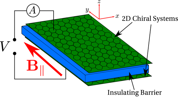
Figure 1: Schematics of the vertical tunneling structure considered in this work. Two parallel chiral two-dimensional electron systems are separated by a uniform barrier. A magnetic field applied parallel to the barrier is used to tune resonances in the tunneling conductance that arise from the requirement of simultaneous energy and momentum conservation.

This article is organized as follows. We begin with a description of the theoretical method in Sec. II. Results obtained for the linear (i.e., zero-bias) magneto-tunneling conductance between various parallel 2D chiral systems are presented in Sec. III. Features arising due to a finite bias are discussed in Sec. IV. The effect of a strong perpendicular magnetic field on tunneling between chiral 2D systems is considered in Sec. V. Using a graphene double-layer system as example, we show in Sec. VI how pseudo-spin-dependent tunnel matrix elements can be extracted from parametric dependencies of the linear tunneling conductance. Section VII contains concluding remarks with a discussion of experimental requirements for verifying our results. Certain technical details are given in Appendices.

II Theoretical description of magneto-tunneling transport

Heterostructures consisting of two tunnel-coupled chiral 2D electron systems are described by a Hamiltonian of the form Vasko (2013)

$$H=\begin{pmatrix}{\mathcal{H}}_{1}&{\mathcal{T}}\\ {\mathcal{T}}^{\dagger}&{\mathcal{H}}_{2}\end{pmatrix}\quad,$$ (1)

where the ${\mathcal{H}}_{1,2}$ are single-particle Hamiltonians acting in the sublattice-related pseudo-spin-1/2 space for electrons in each individual system,  and ${\mathcal{T}}$ is the $2\times 2$ transition matrix that encodes the tunnel coupling between pseudo-spin states from the two systems. Performing a standard calculation Bruus and Flensberg (2004) using linear-response theory for the weak-tunneling limit yields the current-voltage ($I$–$V$) characteristics for tunneling as

$$I(V)=\frac{e}{\hbar}\sum_{\alpha\beta}\int^{\infty}_{-\infty}\frac{d\varepsilon}{2\pi}\,\left[n_{\text{F}}(\varepsilon-eV)-n_{\text{F}}(\varepsilon)\right]$$

$$\hskip 28.45274pt\times\,\mathcal{A}^{(1)}_{\alpha}(\varepsilon)\,\mathcal{A}^{(2)}_{\beta}(\varepsilon-eV)\left|\left\langle\psi^{(1)}_{\alpha}\,\right|{\mathcal{T}}\left|\,\psi^{(2)}_{\beta}\right\rangle\right|^{2}.$$ (2)

The summation index $\alpha$ ($\beta$) runs over the set of quantum numbers for single-particle eigenstates in system 1 (2) and, thus, generally comprises parts related to linear orbital motion, sublattice-related pseudo-spin, real-spin and valley degrees of freedom. $\mathcal{A}^{(m)}_{\alpha}(\varepsilon)$ denotes the spectral function for single-particle excitations with quantum number(s) $\alpha$ in system $m$ at energy $\varepsilon$, $n_{\text{F}}(\varepsilon)$ is the Fermi-Dirac distribution function, and $\big{|}\psi^{(m)}_{\alpha}\big{\rangle}$ is a single-particle eigenstate in system $m$. From the $I$–$V$ characteristics (II), the differential conductance

$$G(V)\equiv\left.\frac{\partial I(V^{\prime})}{\partial V^{\prime}}\right|_{V^{\prime}=V}$$ (3)

can be derived. In the small-bias limit, the tunneling current (II) is proportional to the bias voltage, with the linear conductance $G(0)$ as proportionality factor. Straightforward calculation yields

$$G(0) = \frac{e^{2}}{\hbar}\sum_{\alpha\beta}\int^{\infty}_{-\infty}\frac{d\varepsilon}{2\pi}\,\left(-\frac{\partial n_{\text{F}}(\varepsilon)}{\partial\varepsilon}\right)\,\mathcal{A}^{(1)}_{\alpha}(\varepsilon)\,\mathcal{A}^{(2)}_{\beta}(\varepsilon)$$ (4)

$$\hskip 99.58464pt\times\left|\left\langle\psi^{(1)}_{\alpha}\,\right|{\mathcal{T}}\left|\,\psi^{(2)}_{\beta}\right\rangle\right|^{2}.\quad$$

In a structure with a uniform extended barrier, canonical momentum parallel to the barrier is conserved for tunneling electrons Zheng and MacDonald (1993); Lyo and Simmons (1993); Raichev and Vasko (1996). As a result, the tunneling matrix will be diagonal in the representation of in-plane wave vector ${\bm{\mathrm{k}}}=(k_{x},k_{y})$ and, thus, can be written in the form

$${\mathcal{T}}=\sum_{{\bm{\mathrm{k}}}}|{\bm{\mathrm{k}}}\rangle\langle{\bm{\mathrm{k}}}|\otimes\tau_{\bm{\mathrm{k}}}\quad.$$ (5)

Here $\tau_{\bm{\mathrm{k}}}$ is the momentum-resolved pseudo-spin tunneling matrix that depends on specifics of the heterostructure. Moreover, the single-electron eigenstates in a clean 2D chiral system from the $\gamma$ valley (${\bm{\mathrm{K}}}$ or ${\bm{\mathrm{K^{\prime}}}}$ in graphene) are generally of the form

$$\left|\,\psi_{\gamma,{\bm{\mathrm{k}}},\sigma}\right\rangle=\left|\,{\bm{\mathrm{k}}}\right\rangle\otimes\left|\,\sigma\right\rangle_{\gamma,{\bm{\mathrm{k}}}}\quad,$$ (6)

where $\left|\,\sigma\right\rangle_{\gamma,{\bm{\mathrm{k}}}}$ denotes the eigenstate of pseudo-spin-1/2 projection on a ${\bm{\mathrm{k}}}$-dependent axis. Application of an in-plane magnetic field ${\bm{\mathrm{B}}}_{\parallel}=B_{\parallel}\,{\bm{\mathrm{\hat{b}}}}$ (where ${\bm{\mathrm{\hat{b}}}}$ is the unit vector in ${\bm{\mathrm{B}}}_{\parallel}$ direction) induces a shift between canonical momentum ${\bm{\mathrm{k}}}$ and kinetic momentum ${\bm{\mathrm{\Pi}}}^{(m)}({\bm{\mathrm{k}}},{\bm{\mathrm{B}}}_{\parallel})$ for electrons in system $m$. A convenient choice of gauge yields Zheng and MacDonald (1993); Lyo and Simmons (1993); Raichev and Vasko (1996)

$${\bm{\mathrm{\Pi}}}^{(m)}({\bm{\mathrm{k}}},{\bm{\mathrm{B}}}_{\parallel})={\bm{\mathrm{k}}}+(z_{m}/\ell_{B_{\parallel}}^{2})\,{\bm{\mathrm{\hat{b}}}}\times{\bm{\mathrm{\hat{z}}}}\quad,$$ (7)

where $z_{m}$ is the $z$ coordinate of system $m$ and $\ell_{B}=\sqrt{\hbar/|eB|}$ is the magnetic length. The in-plane magnetic field also modifies the pseudo-spin part of the chiral-2D-electron eigenstates in system $m$, which then read

$$\left|\,\psi^{(m)}_{\gamma,{\bm{\mathrm{k}}},\sigma}({\bm{\mathrm{B}}}_{\parallel})\right\rangle=\left|\,{\bm{\mathrm{k}}}\right\rangle\otimes\left|\,\sigma\right\rangle_{\gamma,{\bm{\mathrm{\Pi}}}^{(m)}({\bm{\mathrm{k}}},{\bm{\mathrm{B}}}_{\parallel})}\quad.$$ (8)

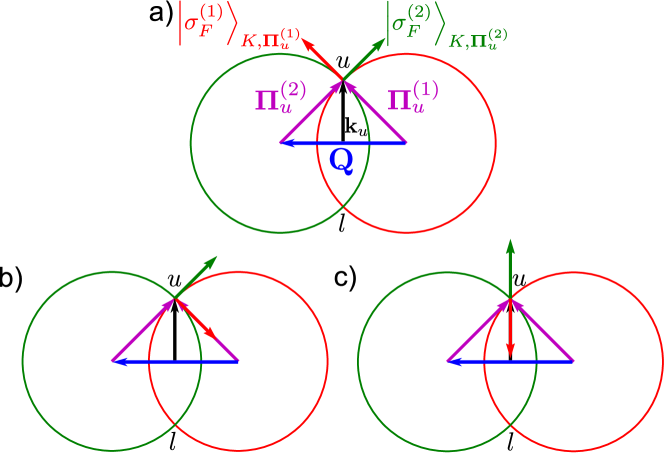
Figure 2: Visualization of constraints due to combined energy and momentum conservation for chiral electrons. An applied in-plane magnetic field results in a shift by ${\bm{\mathrm{Q}}}$ of the Fermi circles associated with the vertically separated 2D conductors. In the zero-bias limit, tunneling can only occur for states at intersection points of the Fermi surfaces. For one of the latter, the kinetic wave vectors and ${\bm{\mathrm{K}}}$-valley pseudo-spin states are indicated for the case of tunneling between a) two n-doped single-layer graphene sheets, b) a p-doped and an n-doped graphene layer, and c) two n-doped bilayer graphene sheets.

Inserting (5) and (8) into the expression (4), using $\mathcal{A}^{(m)}_{\alpha}(\varepsilon)=2\pi\delta\big{(}\varepsilon-\varepsilon^{(m)}_{\alpha}\big{)}$ as is applicable for noninteracting electrons with single-particle energies $\varepsilon^{(m)}_{\alpha}$ in the absence of disorder, and taking the zero-temperature limit yields the linear conductance per unit area as

$$\frac{G(0)}{A}=\frac{g_{\text{s}}e^{2}}{\hbar}\sum_{\gamma}2\pi\,\rho_{\text{F}}^{(1)}\,\rho_{\text{F}}^{(2)}\,\left[\left|\Gamma_{\text{u}}^{(\gamma)}\right|^{2}+\left|\Gamma_{\text{l}}^{(\gamma)}\right|^{2}\right]$$

$$\hskip 2.84544pt\times\frac{\Theta\left(|{\bm{\mathrm{Q}}}|-\left|k_{\text{F}}^{(1)}-k_{\text{F}}^{(2)}\right|\right)\Theta\left(k_{\text{F}}^{(1)}+k_{\text{F}}^{(2)}-|{\bm{\mathrm{Q}}}|\right)}{\sqrt{\left[\left(k_{\text{F}}^{(1)}+k_{\text{F}}^{(2)}\right)^{2}-Q^{2}\right]\left[Q^{2}-\left(k_{\text{F}}^{(1)}-k_{\text{F}}^{(2)}\right)^{2}\right]}}\,.$$ (9)

Here $g_{\text{s}}=2$ is the real-spin degeneracy, $\rho_{\text{F}}^{(m)}$ the density of states at the Fermi energy in system $m$ not including real-spin or valley degrees of freedom, $k_{\text{F}}^{(m)}$ is the Fermi wave vector in system $m$, ${\bm{\mathrm{Q}}}=[(z_{2}-z_{1})/\ell_{B_{\parallel}}^{2}]\,{\bm{\mathrm{\hat{b}}}}\times{\bm{\mathrm{\hat{z}}}}$, and

$$\Gamma_{\text{u/l}}^{(\gamma)}=\,_{\gamma,{\bm{\mathrm{\Pi}}}^{(1)}_{\text{u/l}}}\!\!\left\langle\sigma^{(1)}_{\text{F}}\,\right|\tau_{{\bm{\mathrm{k}}}_{\text{u/l}}}\left|\,\sigma^{(2)}_{\text{F}}\right\rangle_{\!\gamma,{\bm{\mathrm{\Pi}}}^{(2)}_{\text{u/l}}}$$ (10)

are pseudo-spin tunnel matrix elements between states associated with the two intersection points (labelled u and l, respectively) of the two systems’ shifted Fermi circles. See Fig. 2 for an illustration. The canonical and kinetic wave vectors for each of these intersection points can be found from the conditions

$$\left|{\bm{\mathrm{\Pi}}}^{(m)}_{\text{u/l}}\right| = k_{\text{F}}^{(m)}\quad,$$ (11a)

$${\bm{\mathrm{\Pi}}}^{(1)}_{\text{u/l}}-{\bm{\mathrm{\Pi}}}^{(2)}_{\text{u/l}} = {\bm{\mathrm{Q}}}\quad,$$ (11b)

$${\bm{\mathrm{k}}}_{\text{u/l}} = \frac{1}{2}\left({\bm{\mathrm{\Pi}}}^{(1)}_{\text{u/l}}+{\bm{\mathrm{\Pi}}}^{(2)}_{\text{u/l}}-\frac{z_{1}+z_{2}}{\ell_{B_{\parallel}}^{2}}\,{\bm{\mathrm{\hat{b}}}}\times{\bm{\mathrm{\hat{z}}}}\right)\,.\quad$$ (11c)

Furthermore, the projection quantum numbers $\sigma_{\text{F}}^{(m)}$ are determined by the type of charge carriers (electrons or holes) that are present in system $m$: $\sigma_{\text{F}}^{(m)}=+$ ($-$) if system $m$ is n-doped (p-doped).

To be specific, we assume from now on that the pseudo-spin tunneling matrix $\tau_{\bm{\mathrm{k}}}\equiv\tau$ is a constant matrix and use the general parameterization

$$\tau=\left(\tau_{0}\,\sigma_{0}+\tau_{x}\,\sigma_{x}+\tau_{y}\,\sigma_{y}+\tau_{z}\,\sigma_{z}\right)/\sqrt{2}$$ (12)

with, in general, complex numbers $\tau_{j}$ that encode the quantum transfer amplitudes for various possible tunneling processes. For example, $\tau_{0}$ is determined by pseudo-spin-conserving tunneling processes. Introducing a materials-specific conductance unit

$$G_{0}=\frac{g_{\text{s}}g_{\text{v}}e^{2}}{2\pi\hbar}\,\mathrm{Tr}\left[\tau^{\dagger}\tau\right]\,\frac{4\pi^{2}\rho_{\text{F}}^{(1)}\rho_{\text{F}}^{(2)}}{k_{\text{F}}^{(1)}k_{\text{F}}^{(2)}}\,A\quad,$$ (13)

where $g_{\text{v}}$ is the degeneracy factor associated with the valley degree of freedom, enables us to express the magnet-tunneling conductance in a universal form. As an example, and for future comparison, we quote the result obtained Zheng and MacDonald (1993); Raichev and Vasko (1996) for the linear tunneling conductance between two parallel ordinary 2D electron systems with equal density and, hence, same Fermi wave vector $k_{\text{F}}^{(1)}=k_{\text{F}}^{(2)}\equiv\bar{k}_{\text{F}}$:

$$\frac{G^{(\text{ord})}(0)}{G_{0}}=\frac{4\bar{k}_{\text{F}}^{2}}{Q\,\sqrt{4\bar{k}_{\text{F}}^{2}-Q^{2}}}\,\,\Theta(2\bar{k}_{\text{F}}-Q)\quad.$$ (14)

III Linear magneto-tunneling conductance for chiral 2D systems

Results given below have been obtained through application of Eq. (II), with the pseudo-spin-dependent overlap (10) capturing the essential differences between the various 2D chiral systems considered here.

For electrons in a single layer of graphene, the dispersion relation is given by Castro Neto et al. (2009) $\varepsilon_{\gamma,{\bm{\mathrm{k}}},\sigma}^{(\text{slg})}=\sigma\,\hbar v\,k$, and the pseudo-spin states in the ${\bm{\mathrm{K}}}$ and ${\bm{\mathrm{K^{\prime}}}}$ valleys are [$\theta_{\bm{\mathrm{k}}}=\arctan(k_{y}/k_{x})$]

$$\left|\,\sigma\right\rangle_{{\bm{\mathrm{K}}},{\bm{\mathrm{k}}}}^{(\text{slg})}=\frac{1}{\sqrt{2}}\left(\begin{array}[]{c}\mathrm{e}^{-i\frac{\theta_{\bm{\mathrm{k}}}}{2}}\\ \sigma\,\mathrm{e}^{i\frac{\theta_{\bm{\mathrm{k}}}}{2}}\end{array}\right)\,,\,\left|\,\sigma\right\rangle_{{\bm{\mathrm{K^{\prime}}}},{\bm{\mathrm{k}}}}^{(\text{slg})}=\frac{1}{\sqrt{2}}\left(\begin{array}[]{c}\mathrm{e}^{-i\frac{\pi-\theta_{\bm{\mathrm{k}}}}{2}}\\ \sigma\,\mathrm{e}^{i\frac{\pi-\theta_{\bm{\mathrm{k}}}}{2}}\end{array}\right).$$ (15)

We use these states in (10) to find the magneto-tunneling conductance between two parallel n-type graphene layers in terms of $2\bar{k}_{\text{F}}=k_{\text{F}}^{(2)}+k_{\text{F}}^{(1)}$ and $\Delta=\big{|}k_{\text{F}}^{(2)}-k_{\text{F}}^{(1)}\big{|}$ as

$$\frac{G^{(\text{slg})}_{n\leftrightarrow n}(0)}{G_{0}}=\frac{\Theta(Q-\Delta)\Theta(2\bar{k}_{\text{F}}-Q)}{\mathrm{Tr}[\tau^{\dagger}\tau]}\left\{\left[|\tau_{0}|^{2}+|\tau_{\perp}|^{2}\frac{\Delta^{2}}{Q^{2}}\right]\right.$$

$$\times\left.\sqrt{\frac{4\bar{k}_{\text{F}}^{2}-Q^{2}}{Q^{2}-\Delta^{2}}}+\left[|\tau_{z}|^{2}+|\tau_{\|}|^{2}\frac{4\bar{k}_{\text{F}}^{2}}{Q^{2}}\right]\sqrt{\frac{Q^{2}-\Delta^{2}}{4\bar{k}_{\text{F}}^{2}-Q^{2}}}\right\}.\quad$$ (16a)

Here $$\| \perp \tau_{z}=\tau_{\|}=\tau_{\perp}=0$$ () denotes the in-plane direction parallel (perpendicular) to the magnetic field. In the case of pseudo-spin-conserving tunneling (i.e., ) and equal densities in the two layers, Eq. (16) simplifies to

$$\frac{G^{(\text{slg})}_{n\leftrightarrow n}(0)}{G_{0}}=\frac{\sqrt{4\bar{k}_{\text{F}}^{2}-Q^{2}}}{Q}\,\,\Theta(2\bar{k}_{\text{F}}-Q)\quad.$$ (16b)

When one of the systems is p-type and the other n-type, we find

$$\frac{G^{({\rm slg})}_{n\leftrightarrow p}(0)}{G_{0}}=\frac{\Theta(Q-\Delta)\Theta(2\bar{k}_{F}-Q)}{\mathrm{Tr}[\tau^{\dagger}\tau]}\left\{\left[|\tau_{0}|^{2}+|\tau_{\perp}|^{2}\frac{\Delta^{2}}{Q^{2}}\right]\right.$$

$$\times\left.\sqrt{\frac{Q^{2}-\Delta^{2}}{4\bar{k}_{F}^{2}-Q^{2}}}+\left[|\tau_{z}|^{2}+|\tau_{\|}|^{2}\frac{4\bar{k}_{F}^{2}}{Q^{2}}\right]\sqrt{\frac{4\bar{k}_{F}^{2}-Q^{2}}{Q^{2}-\Delta^{2}}}\right\}$$ (17a)

in the most general case. In effect, the way $$\tau_{0} \tau_{z} \tau_{\|} \tau_{\perp}$$ and enter Eq. (17) is switched as compared with Eq. (16), and the same holds for and . The reason for this is the fact that the pseudo-spin of eigenstates at a given wave vector in the conduction band is opposite to the eigenstate with the same wave vector in the valence band. For conserved pseudo-spin and equal densities, the obtained result

$$\frac{G^{(\text{slg})}_{n\leftrightarrow p}(0)}{G_{0}}=\frac{Q}{\sqrt{4\bar{k}_{\text{F}}^{2}-Q^{2}}}\,\,\Theta(2\bar{k}_{\text{F}}-Q)$$ (17b)

coincides with the one found for tunneling between parallel surfaces of a topological insulator Pershoguba and Yakovenko (2012).

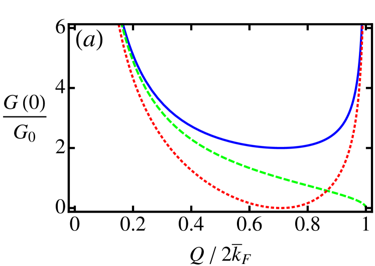
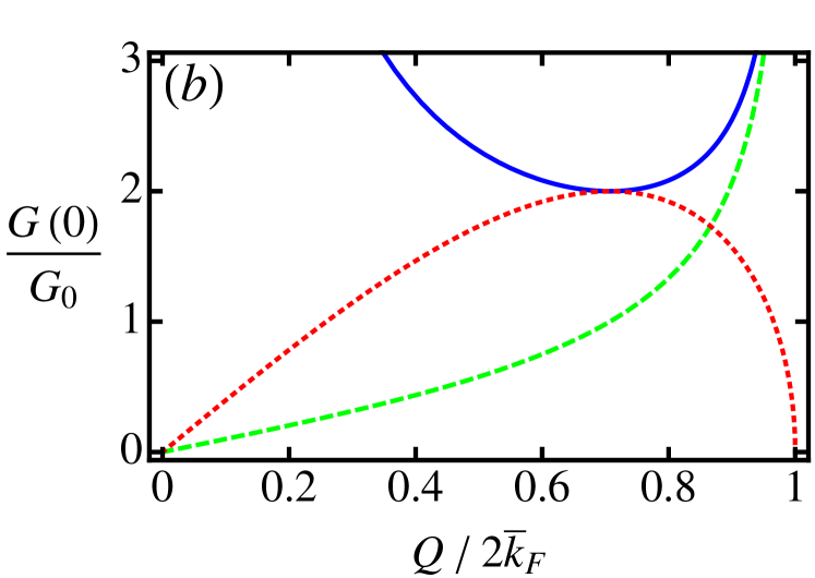
Figure 3: Linear magneto-tunneling conductances between parallel ordinary 2D electron systems (blue solid curves), single-layer graphene sheets (green dashed curves), and bilayer-graphene sheets (red dotted curves) through a pseudo-spin-conserving barrier. $Q=d/\ell_{B_{\|}}^{2}$ is the wave-vector boost induced by a magnetic field of magnitude $B_{\|}$ parallel to the two 2D systems, with $d$ denoting the latters’ vertical separation and $\ell_{B_{\|}}=\sqrt{\hbar/|eB_{\|}|}$ the magnetic length. Panel (a) [(b)] shows results for the case when tunneling occurs between two n-type layers [between an n-type and a p-type layer] with equal density. The pseudo-spin structure of chiral electron states in single-layer and bilayer graphene is the origin of the strongly modified magnetic-field dependences of the tunneling conductance as compared with the ordinary 2D-electron case.

Electrons in a graphene bilayer McCann and Fal’ko (2006) have energy dispersion $\varepsilon_{\gamma,{\bm{\mathrm{k}}},\sigma}^{(\text{blg})}=\sigma\,\hbar^{2}k^{2}/(2M)$ and pseudo-spin states

$$\left|\,\sigma\right\rangle_{{\bm{\mathrm{K}}},{\bm{\mathrm{k}}}}^{(\text{blg})}=\frac{1}{\sqrt{2}}\left(\begin{array}[]{c}\mathrm{e}^{i\theta_{\bm{\mathrm{k}}}}\\ -\sigma\mathrm{e}^{-i\theta_{\bm{\mathrm{k}}}}\end{array}\right)\,,\,\left|\,\sigma\right\rangle_{{\bm{\mathrm{K^{\prime}}}},{\bm{\mathrm{k}}}}^{(\text{blg})}=\frac{1}{\sqrt{2}}\left(\begin{array}[]{c}\mathrm{e}^{-i\theta_{\bm{\mathrm{k}}}}\\ -\sigma\mathrm{e}^{i\theta_{\bm{\mathrm{k}}}}\end{array}\right).$$ (18)

The full analytical expressions for the magneto-tunneling conductance between parallel graphene bilayers are quite cumbersome and therefore given in Eqs. (34) of Appendix A. For equal densities in both systems and a pseudo-spin-conserving barrier, we find

$$\frac{G^{(\text{blg})}_{n\leftrightarrow n}(0)}{G_{0}} = \frac{\left(2\bar{k}_{F}^{2}-Q^{2}\right)^{2}}{\bar{k}_{\text{F}}^{2}\,Q\,\sqrt{4\bar{k}_{F}^{2}-Q^{2}}}\,\,\Theta(2\bar{k}_{\text{F}}-Q)\quad,$$ (19a)

$$\frac{G^{(\text{blg})}_{n\leftrightarrow p}(0)}{G_{0}} = \frac{Q\,\sqrt{4\bar{k}_{\text{F}}^{2}-Q^{2}}}{\bar{k}_{\text{F}}^{2}}\,\,\Theta(2\bar{k}_{\text{F}}-Q)\quad.$$ (19b)

Figure 3 illustrates the drastically different features in the linear magneto-tunneling characteristics for single-layer and bilayer graphene as compared with the ordinary 2D-electron-gas case. For definiteness, the case of a pseudo-spin-conserving barrier is exhibited. The overall suppression of tunneling transport between chiral 2D systems is a consequence of the, in general, misaligned pseudo-spin polarizations of states where the two systems’ Fermi surfaces intersect. (See Fig. 2.) In particular, pseudo-spin orthogonality leads to the vanishing of $G(0)$ in a system of two n-type single layers (bilayers) of graphene when $Q=2\bar{k}_{\text{F}}$ ($Q=\sqrt{2}\,\bar{k}_{\text{F}}$). The fact that the pseudo-spin for eigenstates with opposite sign of the energy is reversed results in the interchange of minima and maxima/divergences in $G(0)$ for tunneling between an n-type and a p-type layer as compared with the case of tunneling between two n-type layers. The magneto-tunneling conductance of the ordinary 2D electron system is reached whenever the pseudo-spins of tunneling states are aligned, e.g., for $Q=\sqrt{2}\,\bar{k}_{\text{F}}$ in tunneling between an n-type and a p-type graphene bilayer. The possibility to have pseudo-spin flipped in a tunneling process enables an even richer structure for tunneling transport, which is captured for the completely general case by the formulae given in Eqs. (16) and (17) [Eqs. (34)] for the single-layer [bilayer] graphene case.

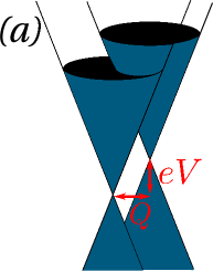
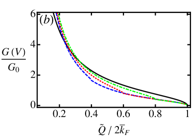
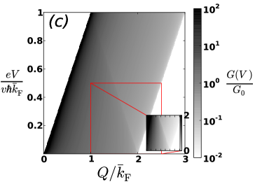
Figure 4: Magneto-tunneling between parallel single-layer graphene sheets at finite bias. (a) The two systems’ Dirac-cone dispersions are shifted with respect to each other by $Q$ ($eV$) in wave-vector (energy) direction due to an applied in-plane magnetic field (bias voltage). Tunneling is possible for states where the conical surfaces intersect, if the state is occupied in one layer and unoccupied in the other. (b) Differential tunneling conductance $G(V)$ for the case when both layers have equal n-type carrier density, plotted as a function of $\tilde{Q}=Q-eV/(\hbar v)$ for $eV=0$ (black solid curve), $0.2\,\hbar v\bar{k}_{\text{F}}$ (green dot-dashed curve), $0.4\,\hbar v\bar{k}_{\text{F}}$ (red dotted curve), and $0.6\,\hbar v\bar{k}_{\text{F}}$ (blue dashed curve). $G(V)$ diverges at $\tilde{Q}=0$ and exhibits square-root-like features at $\tilde{Q}=2\bar{k}_{\text{F}}-2eV/(\hbar v)$ and $\tilde{Q}=2\bar{k}_{\text{F}}$. (c) Logarithmic gray-scale plot of the differential tunneling conductance. The divergence at $eV=\hbar vQ$ and the conical feature with apex at $Q=2\bar{k}_{\text{F}}$ constitute direct measures for the energy dispersion of charge carriers in single-layer graphene.

In contrast to single-layer and bilayer graphene, which are conductors, a single layer of MoS₂ is a semiconducting 2D material. The electronic dispersion is Xiao et al. (2012); Kormányos et al. (2013) $\varepsilon_{\gamma,{\bm{\mathrm{k}}},\sigma}^{(\text{mos})}=\sigma\,\hbar v\sqrt{k^{2}+k_{\Delta}^{2}}$, with constant $k_{\Delta}>0$, and using the abbreviation $\zeta_{k}=k_{\Delta}/\sqrt{k^{2}+k_{\Delta}^{2}}$, the pseudo-spin states can be expressed as

$$\left|\,\sigma\right\rangle_{{\bm{\mathrm{K}}},{\bm{\mathrm{k}}}}^{(\text{mos})}=\left(\begin{array}[]{c}\sqrt{\frac{1+\sigma\zeta_{k}}{2}}\,\mathrm{e}^{-i\frac{\theta_{\bm{\mathrm{k}}}}{2}}\\ \sigma\sqrt{\frac{1-\sigma\zeta_{k}}{2}}\,\mathrm{e}^{i\frac{\theta_{\bm{\mathrm{k}}}}{2}}\end{array}\right)\,\,,$$ (22)

$$\hskip 71.13188pt\left|\,\sigma\right\rangle_{{\bm{\mathrm{K^{\prime}}}},{\bm{\mathrm{k}}}}^{(\text{mos})}=\left(\begin{array}[]{c}\sqrt{\frac{1+\sigma\zeta_{k}}{2}}\,\mathrm{e}^{-i\frac{\pi-\theta_{\bm{\mathrm{k}}}}{2}}\\ \sigma\sqrt{\frac{1-\sigma\zeta_{k}}{2}}\,\mathrm{e}^{i\frac{\pi-\theta_{\bm{\mathrm{k}}}}{2}}\end{array}\right).\quad$$ (25)

The most general expression for the linear magneto-tunneling conductance between parallel single-layer MoS₂ systems is very complicated, and even the result for a pseudo-spin-conserving barrier is so long that it has been relegated to Appendix A [see Eqs. (35)]. If in addition the densities in both layers are equal, we find for the two doping configurations

$$\frac{G^{(\text{mos})}_{n\leftrightarrow n}(0)}{G_{0}} = \left(\frac{\sqrt{4\bar{k}_{\text{F}}^{2}-Q^{2}}}{Q}+\frac{\zeta_{\bar{k}_{\text{F}}}^{2}Q}{\sqrt{4\bar{k}_{\text{F}}^{2}-Q^{2}}}\right)$$ (26a)

$$\hskip 71.13188pt\times\,\Theta(2\bar{k}_{\text{F}}-Q)\,,$$

$$\frac{G^{(\text{mos})}_{n\leftrightarrow p}(0)}{G_{0}} = \frac{\big{(}1-\zeta_{\bar{k}_{\text{F}}}^{2}\big{)}Q}{\sqrt{4\bar{k}_{\text{F}}^{2}-Q^{2}}}\,\,\Theta(2\bar{k}_{\text{F}}-Q)\quad.$$ (26b)

As expected, the behavior of MoS₂ in the limit $\zeta_{k}\to 0$ is the same as that exhibited by single-layer graphene. See Eqs. (16b) and (17b). For $\zeta_{k}\to 1$, $G^{(\text{mos})}_{n\leftrightarrow n}(0)$ recovers the result (14) found for an ordinary 2D electron system, whereas pseudo-spin conservation causes $G^{(\text{mos})}_{n\leftrightarrow p}(0)$ to vanish.

IV Magneto-tunneling at finite bias

Application of the general formula (II) to momentum-resolved tunneling between parallel 2D electron systems in the zero-temperature limit and without disorder yields the general expression

$$I(V)=\frac{1}{e}\int_{\varepsilon_{\text{F}}}^{\varepsilon_{\text{F}}+eV}\,d\varepsilon\,\,\,\tilde{G}(\varepsilon,V)\quad.$$ (27)

Here $\varepsilon_{\text{F}}$ is the Fermi energy of the 2D system whose subband edge (or neutrality point) is taken as the zero of energy. The function $\tilde{G}(\varepsilon,V)$ corresponds to the linear tunneling conductance between the two 2D systems when the chemical potential is equal to $\varepsilon$ and $eV$ has been added to the zero-bias subband-edge splitting.

For illustration of the general principle, we focus here on the special case of pseudo-spin-conserving tunneling between two n-type single-layer graphene sheets with equal carrier densities. It is then straightforward to find

$$\tilde{G}(\varepsilon,V) = G_{0}\,\,\sqrt{\frac{(2\varepsilon-eV)^{2}-(\hbar vQ)^{2}}{(\hbar vQ)^{2}-(eV)^{2}}}$$ (28)

$$\hskip 2.84544pt\times\,\Theta\left(|2\varepsilon-eV|-\hbar vQ\right)\Theta(\hbar vQ-|eV|)\quad$$

by specializing the expression (16) to the situation with $\tau_{\perp,\|,z}=0$ as well as making the substitutions $2\bar{k}_{\text{F}}\to(2\varepsilon-eV)/(\hbar v)$ and $\Delta\to eV/(\hbar v)$. Calculation of the current using (27) and taking the derivative with respect to $V$ yields the differential magneto-tunneling conductance $G(V)$ shown in Fig. 4. It switches on with a divergence when $Q=|eV|/(\hbar v)$ and also exhibits features for $Q=2\bar{k}_{\text{F}}\pm|eV|/(\hbar v)$, which mirror the characteristic switching-off behavior seen in the linear magneto-tunneling conductance between graphene layers at $Q=2\bar{k}_{\text{F}}$ [see the green dashed curve in Fig. 3(a)].

Characteristic features in the differential tunneling conductance between ordinary (non-chiral) 2D electron systems have been shown to provide a direct image of the electronic dispersion relation Rainer et al. (1995); Lyo et al. (2006); Bielejec et al. (2006). The same applies to magneto-tunneling at finite bias between chiral 2D electron systems, except that the type of feature (e.g., divergence, or vanishing) of the differential conductance associated with a dispersion branch is determined by pseudo-spin overlaps. For example, in contrast to the ordinary 2D-electron case where the individual systems’ dispersions are imaged by peaks in the $Q$-dependence of $G(V)$, certain dispersion branches from single-layer graphene sheets are drawn by a square-root-like turning-off behavior in magneto-tunneling transport. See Fig. 4.

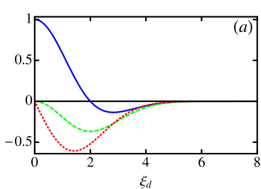
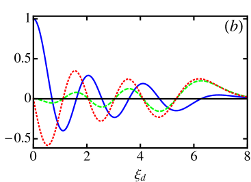
Figure 5: Form factors for tunneling between graphene layers spaced at distance $d$ in a tilted magnetic field ${\bm{\mathrm{B}}}=({\bm{\mathrm{B}}}_{\|},B_{\perp})$, plotted as a function of the parameter $\xi_{d}=(d/\ell_{B_{\perp}})(B_{\|}/B_{\perp})$. See Eq. (29). Panel (a) [(b)] shows $\mathcal{F}^{(+)}_{\nu}(\xi_{d})$ (blue solid curve), $\mathcal{F}^{(-)}_{\nu}(\xi_{d})$ (green dashed curve), and $\mathcal{F}^{(\perp)}_{\nu}(\xi_{d})$ (red dotted curve) for $\nu=1$ [$\nu=6$]. Note the limiting behavior for $\xi_{d}\to 0$ and the oscillatory behavior for cases with $\nu>1$.

V Magneto-tunneling between Landau-quantized graphene layers

The linear tunneling conductance between two chiral 2D electron systems in the presence of a non-vanishing perpendicular magnetic-field component can be found by straightforward application of the general formula (4). Here we discuss in greater detail the case of parallel single layers of graphene. Using the form (5) for the tunneling matrix and Landau-level eigenstates and -energies for graphene Castro Neto et al. (2009); Goerbig (2011), we find analytic results presented in detail in Appendix B. As previously, we focus on the zero-temperature limit and a system without disorder. (Both of these assumptions can be relaxed straightforwardly in principle, resulting in the usual smoothening of resonant features.) To illustrate the effects arising from pseudo-spin dependence, we consider $G(0)$ for the special case when both layers have equal density:

$$G^{(\mathrm{LLg})}_{n\leftrightarrow n}(0) = \frac{g_{\text{s}}g_{\text{v}}e^{2}}{\hbar}\,\frac{A}{\hbar^{2}v^{2}}\,\nu_{\text{F}}\sum_{\nu_{1},\nu_{2}=1}^{\infty}\delta\left(\nu_{\text{F}}-\nu_{1}\right)\delta\left(\nu_{\text{F}}-\nu_{2}\right)\left[\left|\tau_{0}\,\mathcal{F}^{(+)}_{\nu_{1}}(\xi_{d})+\tau_{\perp}\,\mathcal{F}^{(\perp)}_{\nu_{1}}(\xi_{d})\right|^{2}+\left|\tau_{z}\,\mathcal{F}^{(-)}_{\nu_{1}}(\xi_{d})\right|^{2}\right]\,\,,$$ (29a)

$$G^{(\mathrm{LLg})}_{n\leftrightarrow p}(0) = \frac{g_{\text{s}}g_{\text{v}}e^{2}}{\hbar}\,\frac{A}{\hbar^{2}v^{2}}\,\nu_{\text{F}}\sum_{\nu_{1},\nu_{2}=1}^{\infty}\delta\left(\nu_{\text{F}}-\nu_{1}\right)\delta\left(\nu_{\text{F}}-\nu_{2}\right)\left[\left|\tau_{0}\,\mathcal{F}^{(-)}_{\nu_{1}}(\xi_{d})\right|^{2}+\left|\tau_{\|}\,\mathcal{F}^{(\perp)}_{\nu_{1}}(\xi_{d})+\tau_{z}\,\mathcal{F}^{(+)}_{\nu_{1}}(\xi_{d})\right|^{2}\right]\,\,.$$ (29b)

Here $\nu_{\text{F}}$ is the Landau level at the Fermi energy, and the dependence on the in-plane magnetic-field component is governed by form factors $\mathcal{F}^{(\pm,\perp)}(\xi_{d})$ through the parameter $\xi_{d}=(d/\ell_{B_{\perp}})(B_{\|}/B_{\perp})$. See Fig. 5 and explicit mathematical expressions given in Appendix B. The oscillatory behavior as a function of $B_{\|}$ exhibited by the form factors originates from conservation of canonical momentum, which restricts tunneling to Landau-level eigenstates with $B_{\|}$-dependent displacement of their guiding-center locations Raichev and Vasko (1997); Lyo (1998). The linear conductance oscillates also as a function of $B_{\perp}$ because of the Landau-quantization of eigenenergies in 2D electron systems Smoliner et al. (1989a); Raichev and Vasko (1997); Lyo (1998).

The chiral nature of charge carriers in graphene is manifested in a number of differences with respect to the case of an ordinary 2D electron system that was studied, e.g., in Refs. Raichev and Vasko, 1997; Lyo, 1998. Instead of just one form factor that depends on the in-plane field component Raichev and Vasko (1997); Lyo (1998), there are four different form factors in the graphene case, each associated with an independent contribution $\propto\tau_{j}$ to the, in general, pseudo-spin-dependent tunneling matrix. If both graphene layers have equal density, one such form factor vanishes identically. In the limit $B_{\|}\to 0$, only one form factor remains finite, and the linear tunneling conductance becomes proportional to $|\tau_{0}|^{2}$ ($|\tau_{z}|^{2}$) for a system with two n-type layers (one n-type and one p-type layer). Thus linear tunneling transport between Landau-quantized graphene layers enables the direct extraction of pseudo-spin-dependent tunneling matrix elements. This feature will aid in our proposed scheme to extract quantitative information about the pseudo-spin properties of the vertical heterostructure, which is described in the following Section.

VI How to extract the pseudo-spin structure of the tunneling matrix

Our above considerations have shown how tunneling transport between chiral 2D electron systems is strongly dependent on the pseudo-spin structure of the tunnel coupling. As pseudo-spin is related to sub-lattice position, a full parametric study of the tunneling conductance could be employed to yield information about morphological details of the vertical heterostructure. While any type of chiral 2D system lends itself to such an investigation, we describe below an approach that works for two parallel single layers of graphene.

Measurement of the magneto-tunneling conductance between two graphene layers as a function of the externally adjustable parameters $Q$, $\bar{k}_{\text{F}}$ and $\Delta$ makes it possible to extract information about the tunneling matrix $\tau$ given in Eq. (12). This can be done because, according to Eq. (16), the function

$$F(Q,\bar{k}_{\text{F}},\Delta)=\frac{2\pi\hbar G(0)}{g_{\text{s}}g_{\text{v}}e^{2}}\,Q^{2}\sqrt{(4\bar{k}_{\text{F}}^{2}-Q^{2})(Q^{2}-\Delta^{2})}$$ (30a)

is a homogeneous polynomial of its arguments,

$$F(Q,\bar{k}_{\text{F}},\Delta)\equiv-c_{1}\,Q^{4}+c_{2}\,Q^{2}\bar{k}_{\text{F}}^{2}-c_{3}\,Q^{2}\Delta^{2}+c_{4}\,\bar{k}_{\text{F}}^{2}\Delta^{2}\,,$$ (30b)

with coefficients

$$c_{1} = \frac{A\left(|\tau_{0}|^{2}-|\tau_{z}|^{2}\right)}{\hbar^{2}v^{2}}\,\,\,,\,\,\,c_{2}=4\,\frac{A\left(|\tau_{0}|^{2}+|\tau_{\|}|^{2}\right)}{\hbar^{2}v^{2}}\,,$$

$$c_{3} = \frac{A\left(|\tau_{\perp}|^{2}+|\tau_{z}|^{2}\right)}{\hbar^{2}v^{2}}\,\,,\,\,c_{4}=4\,\frac{A\left(|\tau_{\perp}|^{2}-|\tau_{\|}|^{2}\right)}{\hbar^{2}v^{2}}\,.\quad$$ (30c)

Performing fits of the obtained data to the polynomial form (30b) yields the coefficients $c_{j}$. For example, a possible strategy could be to start with measuring $G(0)$ as a function of $Q$ for equal densities in the layers and using the form of $F(Q,\bar{k}_{\text{F}},0)$ to determine $c_{1}$ and $c_{2}$. Fixing then a particular value of $\bar{k}_{\text{F}}$ and $\Delta\neq 0$, varying only $Q$ and considering the combination $F(Q,\bar{k}_{\text{F}},\Delta)+c_{1}Q^{2}-c_{2}Q^{2}\bar{k}_{\text{F}}^{2}$ will then enable extraction of $c_{3}$ and $c_{4}$ from a fit to this quantity’s $Q$ dependence. A first reality check for the theory proposed here would be to demonstrate the relation $c_{2}+c_{4}=4(c_{1}+c_{3})$.

The fact that the coefficients $c_{j}$ satisfy a linear relation means that we need an additional independent measurement to determine the magnitudes of tunnel matrix elements. Resonant tunneling transport in a quantizing perpendicular magnetic field for equal densities between the layers can be used for this purpose. Application of Eqs. (29) allows to extract the ratio of $|\tau_{0}|^{2}/|\tau_{z}|^{2}$, assuming that the inelastic scattering time that broadens the tunneling resonances is the same for n-type and p-type graphene layers. Then all magnitudes of tunneling matrix elements can be determined in units of $\hbar^{2}v^{2}/A$.

The freedom to change the in-plane field direction enables further information to be extracted from magneto-tunneling measurements. A general expression for the magnitudes of tunneling matrix elements can be given in terms of the azimuthal angle $\theta_{{\bm{\mathrm{B}}}_{\|}}\equiv\arctan(B_{\|,y}/B_{\|,x})$ of the in-plane magnetic field,

$$|\tau_{\perp}(\theta_{{\bm{\mathrm{B}}}_{\|}})|^{2} = \frac{|\tau_{x}|^{2}+|\tau_{y}|^{2}}{2}+\frac{|\tau_{x}|^{2}-|\tau_{y}|^{2}}{2}\cos(2\theta_{{\bm{\mathrm{B}}}_{\|}})$$ (31a)

$$\hskip 42.67912pt+\,\myRe\mathrm{e}\,\{\tau_{x}\tau_{y}^{\ast}\}\sin(2\theta_{{\bm{\mathrm{B}}}_{\|}})\,\,,\quad$$

$$|\tau_{\|}(\theta_{{\bm{\mathrm{B}}}_{\|}})|^{2} = \frac{|\tau_{x}|^{2}+|\tau_{y}|^{2}}{2}-\frac{|\tau_{x}|^{2}-|\tau_{y}|^{2}}{2}\cos(2\theta_{{\bm{\mathrm{B}}}_{\|}})$$ (31b)

$$\hskip 42.67912pt-\,\myRe\mathrm{e}\,\{\tau_{x}\tau_{y}^{\ast}\}\sin(2\theta_{{\bm{\mathrm{B}}}_{\|}})\,\,.$$

Thus the phase difference between the generally complex-valued matrix elements $\tau_{x}$ and $\tau_{y}$ can be determined from the tunneling-matrix magnitudes found for $\theta_{{\bm{\mathrm{B}}}_{\|}}=0$ and $\theta_{{\bm{\mathrm{B}}}_{\|}}=\pi/4$:

$$\arg(\tau_{x}\tau_{y}^{\ast})=\arccos\left[\frac{|\tau_{\perp}(\frac{\pi}{4})|^{2}-|\tau_{\perp}(\frac{\pi}{4})|^{2}}{2|\tau_{\|}(0)||\tau_{\perp}(0)|}\right]\quad.$$ (32)

VII Discussion and Conclusions

Experimental exploration of the magneto-tunneling characteristics discussed above requires sufficiently large magnetic fields to shift the entire Fermi circle in kinetic-wave-vector space. Specifically, the condition $|z_{2}-z_{1}|\equiv d\geq 2\bar{k}_{\text{F}}\,\ell_{B_{\parallel}^{\mathrm{(max)}}}^{2}$ ensures that the full range of fields over which tunneling occurs can be accessed. For the case of equal density $n=g_{\text{s}}g_{\text{v}}\bar{k}_{\text{F}}^{2}/(4\pi)$ in the two layers, we find

$$B_{\parallel}^{\mathrm{(max)}}\geq\frac{2\pi\hbar}{e}\,\sqrt{\frac{4}{g_{\text{s}}g_{\text{v}}}\frac{n}{\pi d^{2}}}\approx 20\,\mathrm{T}\times\frac{\sqrt{n\,[10^{10}\,\mathrm{cm}^{-2}]}}{d\,[\mathrm{nm}]}\,\,.$$ (33)

As encapsulation of graphene sheets was shown to enable ballistic transport over $\mu$m-scale distances at low carrier densities Dean et al. (2010); Mayorov et al. (2011), devices with $B_{\parallel}^{\mathrm{(max)}}$ within routinely reachable limits should be accessible with current technology.

Inelastic scattering of 2D chiral quasi-particle excitations due to impurities, coupling to phonons, or Coulomb interactions results in their finite lifetime and concomitant broadening of resonant behavior in the magneto-tunneling conductance Zheng and MacDonald (1993); Lyo and Simmons (1993); Raichev and Vasko (1996); Jungwirth and MacDonald (1996); Raichev and Vasko (1997); Lyo (1998). Such effects can be straightforwardly included in the calculation based on Eq. (4) by using the appropriate form of the single-electron spectral function with life-time broadening.

In conclusion, we have derived analytical expressions for the magneto-tunneling conductance between parallel layers of graphene, bilayer graphene, and MoS₂ in the low-temperature limit and in the absence of interactions and disorder. The constraints imposed by simultaneous energy and momentum conservation in the tunneling processes result in characteristic dependencies on in-plane and perpendicular-to-the-plane magnetic fields as well as the bias voltage. The pseudo-spin properties and chirality of charge carriers in the vertically separated layers strongly affect the magneto-tunneling transport features. Based on the additional dependencies on the densities/Fermi wave vectors in each layer, it is possible to determine the pseudo-spin structure of the tunnel barrier. Our work can thus be used to study, and optimize the design of, vertical-tunneling structures between novel two-dimensional (semi-)conductors.

Appendix A Linear magneto-tunneling conductance for bilayer graphene and MoS₂

The general expression for the magneto-tunneling conductance between two n-doped bilayer-graphene layers is found to be

$$\frac{G^{({\rm blg})}_{n\to n}(0)}{G_{0}} = \frac{\Theta(Q-\Delta)\Theta(2\bar{k}_{\text{F}}-Q)}{\mathrm{Tr}[\tau^{\dagger}\tau]}\left\{\frac{\left|\tau_{0}\left(4\bar{k}_{\text{F}}^{2}+\Delta^{2}-2Q^{2}\right)Q^{2}-\tau_{\perp}\left[8\bar{k}_{\text{F}}^{2}\,\Delta^{2}-\left(4\bar{k}_{\text{F}}^{2}+\Delta^{2}\right)Q^{2}\right]\right|^{2}}{Q^{4}\left(4\bar{k}_{\text{F}}^{2}-\Delta^{2}\right)\sqrt{\left(4\bar{k}_{\text{F}}^{2}-Q^{2}\right)\left(Q^{2}-\Delta^{2}\right)}}\right.$$ (34a)

$$\hskip 170.71652pt\left.+\,\,\left|\tau_{\|}\,8\bar{k}_{\text{F}}^{2}\,\Delta^{2}-i\,\tau_{z}\,2Q^{2}\right|^{2}\,\frac{\sqrt{\left(4\bar{k}_{\text{F}}^{2}-Q^{2}\right)\left(Q^{2}-\Delta^{2}\right)}}{Q^{4}\left(4\bar{k}_{\text{F}}^{2}-\Delta^{2}\right)}\right\}\,,\quad$$

whereas the conductance between an n-doped and a p-doped bilayer is given by

$$\frac{G^{({\rm blg})}_{n\to p}(0)}{G_{0}} = \frac{\Theta(Q-\Delta)\Theta(2\bar{k}_{\text{F}}-Q)}{\mathrm{Tr}[\tau^{\dagger}\tau]}\left\{\left|\tau_{0}\,2Q^{2}+\tau_{\perp}\,8\bar{k}_{\text{F}}^{2}\,\Delta^{2}\right|^{2}\frac{\sqrt{\left(4\bar{k}_{\text{F}}^{2}-Q^{2}\right)\left(Q^{2}-\Delta^{2}\right)}}{Q^{4}\left(4\bar{k}_{\text{F}}^{2}-\Delta^{2}\right)}\right.$$ (34b)

$$\hskip 113.81102pt\left.+\,\,\frac{\left|\tau_{\|}\left[8\bar{k}_{\text{F}}^{2}\,\Delta^{2}-\left(4\bar{k}_{\text{F}}^{2}+\Delta^{2}\right)Q^{2}\right]+i\,\tau_{z}\left(4\bar{k}_{\text{F}}^{2}+\Delta^{2}-2Q^{2}\right)Q^{2}\right|^{2}}{Q^{4}\left(4\bar{k}_{\text{F}}^{2}-\Delta^{2}\right)\sqrt{\left(4\bar{k}_{\text{F}}^{2}-Q^{2}\right)\left(Q^{2}-\Delta^{2}\right)}}\right\}\,.\quad$$

Note that, unlike for tunneling between single-layer graphene sheets, the phase of the tunneling matrix plays a role in determining the transport characteristics for tunneling between two bilayer-graphene systems. Furthermore, the conductance obtained for tunneling between two p-type bilayers differs from that found for two n-type bilayers by an opposite sign in the terms involving $\tau_{\perp}$ and $\tau_{z}$.

To discuss magneto-tunneling transport between two parallel single layers of MoS₂, we restrict ourselves to the case of a pseudo-spin-conserving barrier because the fully general formulae are quite cumbersome. We obtain

$$\frac{G^{(\mathrm{mos})}_{n\to n}(0)}{G_{0}} = \frac{\Theta(Q-\Delta)\Theta(2\bar{k}_{\text{F}}-Q)}{4}\left\{\sqrt{\frac{4\bar{k}_{\text{F}}^{2}-Q^{2}}{Q^{2}-\Delta^{2}}}\left[\sqrt{\left(1+\zeta_{k_{\text{F}}^{(1)}}\right)\left(1+\zeta_{k_{\text{F}}^{(2)}}\right)}+\sqrt{\left(1-\zeta_{k_{\text{F}}^{(1)}}\right)\left(1-\zeta_{k_{\text{F}}^{(2)}}\right)}\right]^{2}\right.$$ (35a)

$$\hskip 56.9055pt\left.+\,\,\sqrt{\frac{Q^{2}-\Delta^{2}}{4\bar{k}_{\text{F}}^{2}-Q^{2}}}\left[\sqrt{\left(1+\zeta_{k_{\text{F}}^{(1)}}\right)\left(1+\zeta_{k_{\text{F}}^{(2)}}\right)}-\sqrt{\left(1-\zeta_{k_{\text{F}}^{(1)}}\right)\left(1-\zeta_{k_{\text{F}}^{(2)}}\right)}\right]^{2}\right\}$$

for the case when both layers are n-doped, whereas for tunneling between an n-doped and a p-doped layer, the result

$$\frac{G^{(\mathrm{mos})}_{n\to p}(0)}{G_{0}} = \frac{\Theta(Q-\Delta)\Theta(2\bar{k}_{\text{F}}-Q)}{4}\left\{\sqrt{\frac{4\bar{k}_{\text{F}}^{2}-Q^{2}}{Q^{2}-\Delta^{2}}}\left[\sqrt{\left(1+\zeta_{k_{\text{F}}^{(1)}}\right)\left(1-\zeta_{k_{\text{F}}^{(2)}}\right)}-\sqrt{\left(1-\zeta_{k_{\text{F}}^{(1)}}\right)\left(1+\zeta_{k_{\text{F}}^{(2)}}\right)}\right]^{2}\right.$$ (35b)

$$\hskip 56.9055pt\left.+\,\,\sqrt{\frac{Q^{2}-\Delta^{2}}{4\bar{k}_{\text{F}}^{2}-Q^{2}}}\left[\sqrt{\left(1+\zeta_{k_{\text{F}}^{(1)}}\right)\left(1-\zeta_{k_{\text{F}}^{(2)}}\right)}+\sqrt{\left(1-\zeta_{k_{\text{F}}^{(1)}}\right)\left(1+\zeta_{k_{\text{F}}^{(2)}}\right)}\right]^{2}\right\}$$

is found.

Appendix B Momentum-resolved tunneling between Landau-quantized graphene layers in a tilted field

Using the familiar Landau-level ladder operators defined by $a^{\pm}=\ell_{B_{\perp}}\left(\Pi_{x}\pm i\,\Pi_{y}\right)/(\sqrt{2}\hbar)$, with kinetic momentum ${\bm{\mathrm{\Pi}}}={\bm{\mathrm{p}}}+e\,{\bm{\mathrm{A}}}$ in terms of the magnetic vector potential ${\bm{\mathrm{A}}}$, the single-particle Hamiltonians for the ${\bm{\mathrm{K}}}$ and ${\bm{\mathrm{K^{\prime}}}}\equiv-{\bm{\mathrm{K}}}$ valleys of graphene are given by Castro Neto et al. (2009); Goerbig (2011)

$${\mathcal{H}}_{\pm{\bm{\mathrm{K}}}}(B_{\perp})=\pm\sqrt{2}\,\frac{\hbar v}{\ell_{B_{\perp}}}\begin{pmatrix}0&a^{\mp}\\ a^{\pm}&0\end{pmatrix}\quad.$$ (36)

For definiteness, we choose the Landau gauge ${\bm{\mathrm{A}}}=(-y\,B_{\perp}+z\,B_{\|},0,0)$, where $z$ is the constant ${\bm{\mathrm{\hat{z}}}}$ coordinate of charge carriers in the 2D layer. The energy eigenvalues of ${\mathcal{H}}_{\pm{\bm{\mathrm{K}}}}(B_{\perp})$ are found to be $\epsilon_{\sigma,\nu}=\sigma\,\hbar v\sqrt{2\nu}/\ell_{B_{\perp}}$, where $\nu=0,1,\dots$, and the corresponding eigenstates in the ${\bm{\mathrm{K}}}$ and ${\bm{\mathrm{K^{\prime}}}}$ valleys are Castro Neto et al. (2009); Goerbig (2011)

$$\left|\,\nu,\sigma,\kappa_{x}\right\rangle_{{\bm{\mathrm{K}}}} = \frac{1}{\sqrt{2}}\begin{pmatrix}\sigma\left|\,\nu-1,\kappa_{x}\right\rangle\\ \left|\,\nu,\kappa_{x}\right\rangle\end{pmatrix}\,\,\mbox{for $\nu>0$, and}\,\,\left|\,0,\kappa_{x}\right\rangle_{{\bm{\mathrm{K}}}}=\begin{pmatrix}0\\ \left|\,0,\kappa_{x}\right\rangle\end{pmatrix}\quad,$$ (37a)

$$\left|\,\nu,\sigma,\kappa_{x}\right\rangle_{{\bm{\mathrm{K^{\prime}}}}} = \frac{1}{\sqrt{2}}\begin{pmatrix}\left|\,\nu,\kappa_{x}\right\rangle\\ \sigma\left|\,\nu-1,\kappa_{x}\right\rangle\end{pmatrix}\,\,\mbox{for $\nu>0$, and}\,\,\left|\,0,\kappa_{x}\right\rangle_{{\bm{\mathrm{K^{\prime}}}}}=\begin{pmatrix}\left|\,0,\kappa_{x}\right\rangle\\ 0\end{pmatrix}\quad.$$ (37b)

Here the real-space Landau-level eigenstates satisfy $a^{+}a^{-}\left|\,\nu,\kappa_{x}\right\rangle=\nu\left|\,\nu,\kappa_{x}\right\rangle$, with the quantum number $\kappa_{x}\equiv k_{x}+z/\ell_{B_{\|}}^{2}$ being related to the cyclotron-orbit guiding-center position in $y$ direction. In the following, it will be useful to note the mathematical relation Hu and MacDonald (1992); Lyo (1998)

$$\left\langle\nu,\kappa_{x}\,|\,\nu^{\prime},\kappa_{x}^{\prime}\right\rangle=\delta_{k_{x},k_{x}^{\prime}}\,\,(-1)^{\nu_{>}-\nu_{<}}\,\left(\frac{\nu_{<}!}{\nu_{>}!}\right)^{\frac{1}{2}}\left(\frac{\xi^{2}}{2}\right)^{\frac{\nu_{>}-\nu_{<}}{2}}\mathrm{e}^{-\frac{\xi^{2}}{4}}\,\,L_{\nu_{<}}^{\nu_{>}-\nu_{<}}\left(\frac{\xi^{2}}{2}\right)\quad,$$ (38)

where $\nu_{<(>)}=\mathrm{min(max)}\{\nu,\nu^{\prime}\}$, $\xi=(|z-z^{\prime}|/\ell_{B_{\perp}})(B_{\|}/B_{\perp})$, and $L_{n}^{n^{\prime}}(\cdot)$ is the generalized Laguerre polynomial.

Using the Landau-level eigenstates and eigenenergies for calculating the linear tunneling conductance from Eq. (4), we find

$$G^{(\mathrm{LLg})} = \frac{g_{\text{s}}g_{\text{v}}e^{2}}{\hbar}\,\frac{A}{\hbar^{2}v^{2}}\,\sqrt{\nu_{\text{F}}^{(1)}\left(\nu_{\text{F}}^{(1)}+\Delta\nu_{\text{F}}\right)}\sum_{\nu_{1},\nu_{2}=1}^{\infty}\delta\left(\nu_{\text{F}}^{(1)}-\nu_{1}\right)\delta\left(\nu_{\text{F}}^{(1)}+\Delta\nu_{\text{F}}-\nu_{2}\right)$$ (39)

$$\hskip 156.49014pt\times\left[\left|\tau_{0}\,F^{(0)}_{\nu_{1}\nu_{2}}(\xi_{d})+\tau_{x}\,F^{(x)}_{\nu_{1}\nu_{2}}(\xi_{d})\right|^{2}+\left|\tau_{y}\,F^{(y)}_{\nu_{1}\nu_{2}}(\xi_{d})+\tau_{z}\,F^{(z)}_{\nu_{1}\nu_{2}}(\xi_{d})\right|^{2}\right]\,\,,\quad$$

where we denote the Landau level at the Fermi energy in layer $j$ by $\nu_{\text{F}}^{(j)}$, $\Delta\nu_{\text{F}}=\nu_{\text{F}}^{(2)}-\nu_{\text{F}}^{(1)}$, and $\xi_{d}\equiv\xi$ for $|z-z^{\prime}|\to d$ where $d$ is the vertical separation between the two graphene layers. Terms with $\nu_{1}=0$ or $\nu_{2}=0$ have been omitted from the sum on the r.h.s of (39) because theses have a vanishing prefactor. It should be noted that such terms would, however, contribute if our assumption of purely elastic scattering were to be relaxed. The $F^{(j)}_{\nu_{1}\nu_{2}}(\xi)$ are form factors describing the effect of the in-plane magnetic field. For $\nu_{>}\neq\nu_{<}$, we find

$$F^{(0)}_{\nu_{1}\nu_{2}}(\xi) = \frac{1}{2}\,\left(\frac{\nu_{<}!}{\nu_{>}!}\right)^{\frac{1}{2}}\left(\frac{\xi^{2}}{2}\right)^{\frac{\nu_{>}-\nu_{<}}{2}}\mathrm{e}^{-\frac{\xi^{2}}{4}}\left[L_{\nu_{<}}^{\nu_{>}-\nu_{<}}\left(\frac{\xi^{2}}{2}\right)\pm\sqrt{\frac{\nu_{>}}{\nu_{<}}}\,\,L_{\nu_{<}-1}^{\nu_{>}-\nu_{<}}\left(\frac{\xi^{2}}{2}\right)\right]\,\,,$$ (40a)

$$F^{(x)}_{\nu_{1}\nu_{2}}(\xi) = -\frac{1}{2}\,\left(\frac{\nu_{<}!}{\nu_{>}!}\right)^{\frac{1}{2}}\left(\frac{\xi^{2}}{2}\right)^{\frac{\nu_{>}-\nu_{<}-1}{2}}\mathrm{e}^{-\frac{\xi^{2}}{4}}\left[\sqrt{\nu_{>}}\,\,L_{\nu_{<}}^{\nu_{>}-\nu_{<}-1}\left(\frac{\xi^{2}}{2}\right)\pm\frac{\xi^{2}}{2\sqrt{\nu_{<}}}\,\,L_{\nu_{<}-1}^{\nu_{>}-\nu_{<}+1}\left(\frac{\xi^{2}}{2}\right)\right]\,\,,$$ (40b)

$$F^{(y)}_{\nu_{1}\nu_{2}}(\xi) = -\frac{i}{2}\,\left(\frac{\nu_{<}!}{\nu_{>}!}\right)^{\frac{1}{2}}\left(\frac{\xi^{2}}{2}\right)^{\frac{\nu_{>}-\nu_{<}-1}{2}}\mathrm{e}^{-\frac{\xi^{2}}{4}}\left[\sqrt{\nu_{>}}\,\,L_{\nu_{<}}^{\nu_{>}-\nu_{<}-1}\left(\frac{\xi^{2}}{2}\right)\mp\frac{\xi^{2}}{2\sqrt{\nu_{<}}}\,\,L_{\nu_{<}-1}^{\nu_{>}-\nu_{<}+1}\left(\frac{\xi^{2}}{2}\right)\right]\,\,,$$ (40c)

$$F^{(z)}_{\nu_{1}\nu_{2}}(\xi) = \frac{1}{2}\,\left(\frac{\nu_{<}!}{\nu_{>}!}\right)^{\frac{1}{2}}\left(\frac{\xi^{2}}{2}\right)^{\frac{\nu_{>}-\nu_{<}}{2}}\mathrm{e}^{-\frac{\xi^{2}}{4}}\left[L_{\nu_{<}}^{\nu_{>}-\nu_{<}}\left(\frac{\xi^{2}}{2}\right)\mp\sqrt{\frac{\nu_{>}}{\nu_{<}}}\,\,L_{\nu_{<}-1}^{\nu_{>}-\nu_{<}}\left(\frac{\xi^{2}}{2}\right)\right]\,\,,$$ (40d)

where the upper (lower) sign of terms applies to tunneling between two n-type layers (an n-type and a p-type layer). When $\nu_{1}=\nu_{2}\equiv\nu$, we have

$$\left.F^{(0)}_{\nu\nu}(\xi)\right|_{n\to n} \equiv \left.F^{(z)}_{\nu\nu}(\xi)\right|_{n\to p}=\mathcal{F}_{\nu}^{(+)}(\xi)\,\,,$$ (41a)

$$\left.F^{(x)}_{\nu\nu}(\xi)\right|_{n\to n} \equiv \left.i\,F^{(y)}_{\nu\nu}(\xi)\right|_{n\to p}=\mathcal{F}_{\nu}^{(\perp)}(\xi)\,\,,$$ (41b)

$$\left.F^{(y)}_{\nu\nu}(\xi)\right|_{n\to n} \equiv \left.F^{(x)}_{\nu\nu}(\xi)\right|_{n\to p}=0\,\,,$$ (41c)

$$\left.F^{(z)}_{\nu\nu}(\xi)\right|_{n\to n} \equiv \left.F^{(0)}_{\nu\nu}(\xi)\right|_{n\to p}=\mathcal{F}_{\nu}^{(-)}(\xi)\,\,,$$ (41d)

with the definitions

$$\mathcal{F}_{\nu}^{(\pm)}(\xi) = \frac{1}{2}\mathrm{e}^{-\frac{\xi^{2}}{4}}\left[L_{\nu}^{0}\left(\frac{\xi^{2}}{2}\right)\pm L_{\nu-1}^{0}\left(\frac{\xi^{2}}{2}\right)\right]\,\,,\quad$$ (42a)

$$\mathcal{F}_{\nu}^{(\perp)}(\xi) = -\mathrm{e}^{-\frac{\xi^{2}}{4}}\sqrt{\frac{\xi^{2}}{2\nu}}L_{\nu-1}^{1}\left(\frac{\xi^{2}}{2}\right)\,\,.$$ (42b)

In the $B_{\|}=0$ limit (i.e., for $\xi\to 0$), the form factors restrict tunneling to occur between the same or adjacent Landau levels, depending on the pseudo-spin structure of the tunneling matrix.

References

- Wolf (1985) E. L. Wolf, Principles of Electron Tunneling Spectroscopy (Oxford University Press, New York, 1985).
- Smoliner et al. (1989a) J. Smoliner, E. Gornik, and G. Weimann, Phys. Rev. B 39, 12937 (1989a).
- Smoliner et al. (1989b) J. Smoliner, W. Demmerle, G. Berthold, E. Gornik, G. Weimann, and W. Schlapp, Phys. Rev. Lett. 63, 2116 (1989b).
- Eisenstein et al. (1991) J. P. Eisenstein, T. J. Gramila, L. N. Pfeiffer, and K. W. West, Phys. Rev. B 44, 6511 (1991).
- Hayden et al. (1991) R. K. Hayden, D. K. Maude, L. Eaves, E. C. Valadares, M. Henini, F. W. Sheard, O. H. Hughes, J. C. Portal, and L. Cury, Phys. Rev. Lett. 66, 1749 (1991).
- Gennser et al. (1991) U. Gennser, V. P. Kesan, D. A. Syphers, T. P. Smith, S. S. Iyer, and E. S. Yang, Phys. Rev. Lett. 67, 3828 (1991).
- Simmons et al. (1993) J. A. Simmons, S. K. Lyo, J. F. Klem, M. E. Sherwin, and J. R. Wendt, Phys. Rev. B 47, 15741 (1993).
- Patel et al. (1996) N. K. Patel, A. Kurobe, I. M. Castleton, E. H. Linfield, K. M. Brown, M. P. Grimshaw, D. A. Ritchie, G. A. C. Jones, and M. Pepper, Semicond. Sci. Technol. 11, 703 (1996).
- Hasbun (2003) J. E. Hasbun, J. Phys.: Condens. Matter 15, R143 (2003).
- Eugster et al. (1994) C. C. Eugster, J. A. del Alamo, M. J. Rooks, and M. R. Melloch, Appl. Phys. Lett. 64, 3157 (1994).
- Wang et al. (1994) J. Wang, P. H. Beton, N. Mori, L. Eaves, H. Buhmann, L. Mansouri, P. C. Main, T. J. Foster, and M. Henini, Phys. Rev. Lett. 73, 1146 (1994).
- Auslaender et al. (2002) O. M. Auslaender, A. Yacoby, R. de Picciotto, K. W. Baldwin, L. N. Pfeiffer, and K. W. West, Science 295, 825 (2002).
- Bielejec et al. (2005) E. Bielejec, J. A. Seamons, J. L. Reno, and M. P. Lilly, Appl. Phys. Lett. 86, 083101 (2005).
- Vdovin et al. (2000) E. E. Vdovin, A. Levin, A. Patan , L. Eaves, P. C. Main, Y. N. Khanin, Y. V. Dubrovskii, M. Henini, and G. Hill, Science 290, 122 (2000).
- Rainer et al. (1995) G. Rainer, J. Smoliner, E. Gornik, G. Böhm, and G. Weimann, Phys. Rev. B 51, 17642 (1995).
- Lyo et al. (2006) S. Lyo, E. Bielejec, J. Seamons, J. Reno, M. Lilly, and Y. Shim, Physica E 34, 425 (2006).
- Bielejec et al. (2006) E. Bielejec, J. Seamons, J. Reno, S. Lyo, and M. Lilly, Physica E 34, 433 (2006).
- Auslaender et al. (2005) O. M. Auslaender, H. Steinberg, A. Yacoby, Y. Tserkovnyak, B. I. Halperin, K. W. Baldwin, L. N. Pfeiffer, and K. W. West, Science 308, 88 (2005).
- Jompol et al. (2009) Y. Jompol, C. J. B. Ford, J. P. Griffiths, I. Farrer, G. A. C. Jones, D. Anderson, D. A. Ritchie, T. W. Silk, and A. J. Schofield, Science 325, 597 (2009).
- Zülicke (2002) U. Zülicke, Science 295, 810 (2002).
- Raichev and Debray (2003) O. E. Raichev and P. Debray, Phys. Rev. B 67, 155304 (2003).
- Rozhansky and Averkiev (2008) I. V. Rozhansky and N. S. Averkiev, Phys. Rev. B 77, 115309 (2008).
- Governale et al. (2002) M. Governale, D. Boese, U. Zülicke, and C. Schroll, Phys. Rev. B 65, 140403 (2002).
- Raichev and Vasko (2004) O. E. Raichev and F. T. Vasko, Phys. Rev. B 70, 075311 (2004).
- Pershoguba and Yakovenko (2012) S. S. Pershoguba and V. M. Yakovenko, Phys. Rev. B 86, 165404 (2012).
- Britnell et al. (2012a) L. Britnell, R. V. Gorbachev, R. Jalil, B. D. Belle, F. Schedin, A. Mishchenko, T. Georgiou, M. I. Katsnelson, L. Eaves, S. V. Morozov, N. M. R. Peres, J. Leist, A. K. Geim, K. S. Novoselov, and L. A. Ponomarenko, Science 335, 947 (2012a).
- Britnell et al. (2012b) L. Britnell, R. V. Gorbachev, R. Jalil, B. D. Belle, F. Schedin, M. I. Katsnelson, L. Eaves, S. V. Morozov, A. S. Mayorov, N. M. R. Peres, A. H. Castro Neto, J. Leist, A. K. Geim, L. A. Ponomarenko, and K. S. Novoselov, Nano Lett. 12, 1707 (2012b).
- Georgiou et al. (2012) T. Georgiou, R. Jalil, B. D. Belle, L. Britnell, R. V. Gorbachev, S. V. Morozov, Y.-J. Kim, A. Gholinia, S. J. Haigh, O. Makarovsky, L. Eaves, L. A. Ponomarenko, A. K. Geim, K. S. Novoselov, and A. Mishchenko, Nat. Nanotech. 8, 100 (2012).
- Britnell et al. (2013) L. Britnell, R. V. Gorbachev, A. K. Geim, L. A. Ponomarenko, A. Mishchenko, M. T. Greenaway, T. M. Fromhold, K. S. Novoselov, and L. Eaves, Nat. Comms. 4, 1794 (2013).
- Geim and Grigorieva (2013) A. K. Geim and I. V. Grigorieva, Nature (London) 499, 419 (2013).
- Myoung et al. (2013) N. Myoung, K. Seo, S. J. Lee, and G. Ihm, ACS Nano 7, 7021 (2013).
- Castro Neto et al. (2009) A. H. Castro Neto, F. Guinea, N. M. R. Peres, K. S. Novoselov, and A. K. Geim, Rev. Mod. Phys. 81, 109 (2009).
- Feenstra et al. (2012) R. M. Feenstra, D. Jena, and G. Gu, J. Appl. Phys. 111, 043711 (2012).
- Bala Kumar et al. (2012) S. Bala Kumar, G. Seol, and J. Guo, Appl. Phys. Lett. 101, 033503 (2012).
- Vasko (2013) F. T. Vasko, Phys. Rev. B 87, 075424 (2013).
- Note (1) We neglect all electron-electron interactions in this work.
- Bruus and Flensberg (2004) H. Bruus and K. Flensberg, Many-Body Quantum Theory in Condensed Matter Physics: An Introduction (Oxford University Press, Oxford, UK, 2004).
- Zheng and MacDonald (1993) L. Zheng and A. H. MacDonald, Phys. Rev. B 47, 10619 (1993).
- Lyo and Simmons (1993) S. K. Lyo and J. A. Simmons, J. Phys.: Condens. Matter 5, L299 (1993).
- Raichev and Vasko (1996) O. E. Raichev and F. T. Vasko, J. Phys.: Condens. Matter 8, 1041 (1996).
- McCann and Fal’ko (2006) E. McCann and V. I. Fal’ko, Phys. Rev. Lett. 96, 086805 (2006).
- Xiao et al. (2012) D. Xiao, G.-B. Liu, W. Feng, X. Xu, and W. Yao, Phys. Rev. Lett. 108, 196802 (2012).
- Kormányos et al. (2013) A. Kormányos, V. Zólyomi, N. D. Drummond, P. Rakyta, G. Burkard, and V. I. Fal’ko, Phys. Rev. B 88, 045416 (2013).
- Goerbig (2011) M. O. Goerbig, Rev. Mod. Phys. 83, 1193 (2011).
- Raichev and Vasko (1997) O. E. Raichev and F. T. Vasko, J. Phys.: Condens. Matter 9, 1547 (1997).
- Lyo (1998) S. K. Lyo, Phys. Rev. B 57, 9114 (1998).
- Dean et al. (2010) C. R. Dean, A. F. Young, I. Meric, C. Lee, L. Wang, S. Sorgenfrei, K. Watanabe, T. Taniguchi, P. Kim, K. L. Shepard, and J. Hone, Nat. Nanotech. 5, 722 (2010).
- Mayorov et al. (2011) A. S. Mayorov, R. V. Gorbachev, S. V. Morozov, L. Britnell, R. Jalil, L. A. Ponomarenko, P. Blake, K. S. Novoselov, K. Watanabe, T. Taniguchi, and A. K. Geim, Nano Lett. 11, 2396 (2011).
- Jungwirth and MacDonald (1996) T. Jungwirth and A. H. MacDonald, Phys. Rev. B 53, 7403 (1996).
- Hu and MacDonald (1992) J. Hu and A. H. MacDonald, Phys. Rev. B 46, 12554 (1992).