Second-Order Asymptotics for the Classical
Capacity of Image-Additive Quantum Channels

Abstract

We study non-asymptotic fundamental limits for transmitting classical information over memoryless quantum channels, i.e. we investigate the amount of classical information that can be transmitted when a quantum channel is used a finite number of times and a fixed, non-vanishing average error is permissible. In this work we consider the classical capacity of quantum channels that are image-additive, including all classical to quantum channels, as well as the product state capacity of arbitrary quantum channels. In both cases we show that the non-asymptotic fundamental limit admits a second-order approximation that illustrates the speed at which the rate of optimal codes converges to the Holevo capacity as the blocklength tends to infinity. The behavior is governed by a new channel parameter, called channel dispersion, for which we provide a geometrical interpretation.

I Introduction

One of the landmark achievements in quantum information theory is the establishing of the coding theorem for sending classical information across a noisy quantum channel by Holevo holevo98 , and independently by Schumacher-Westmoreland schumacher97  — the so-called HSW theorem. The HSW theorem can be formally stated as follows: Let $\mathcal{W}^{n}$ denote the $n$-fold memoryless composition of the channel $\mathcal{W}$ and let $M^{*}(\mathcal{W}^{n},\varepsilon)$ denote the maximum size of a length-$n$ block code for the channel $\mathcal{W}$ with average error probability $\varepsilon\in(0,1)$. Then, the HSW theorem, together with the weak converse established by Holevo holevo73b in the 1970s (the Holevo bound), asserts that

$$C(\mathcal{W}):=\lim_{\varepsilon\to 0}\liminf_{n\to\infty}\frac{1}{n}\log M^{*}(\mathcal{W}^{n},\varepsilon)=\lim_{n\to\infty}\frac{1}{n}\chi(\mathcal{W}^{n}),$$ (1)

where $\chi(\mathcal{W})$ is the Holevo capacity of the channel. (We define all quantities precisely in the following.) Let us emphasize that the Holevo capacity is generally not additive hastings09 , and we can thus not simplify the limit on the right hand side of (1) without further assumptions.

However, for discrete classical-quantum (c-q) channels, the converse part of HSW theorem was strengthened significantly by Ogawa-Nagaoka ogawa99 and Winter winter99 ; winterthesis who proved the strong converse for discrete memoryless c-q channels, namely

$$\lim_{n\to\infty}\frac{1}{n}\log M^{*}(\mathcal{W}^{n},\varepsilon)=\chi(\mathcal{W})=C(\mathcal{W}),\quad\mbox{for all }\varepsilon\in(0,1).$$ (2)

In the work by Ogawa-Nagaoka ogawa99 , the strong converse was proved using ideas from Arimoto’s strong converse proof arimoto73 for classical channels, which itself was based on techniques to prove Gallager’s random coding error exponent gallager65 . Hence, Ogawa and Nagaoka’s proof ogawa99 also applies to c-q channels whose inputs are not necessarily discrete. Winter’s strong converse proof winter99 , on the other hand, is based on the method of types csiszar98 which is a powerful tool developed in classical information theory for discrete memoryless systems. Winter then combines this method with a suitable discretization of the output space to show the strong converse for non-stationary channels winterthesis . We also mention the work by Hayashi-Nagaoka hayashi03 in which a necessary and sufficient condition was provided for the strong converse property to hold for general (not only memoryless) c-q channels. More recently, Wilde-Winter-Yang wilde13 established that the strong converse, Eq. (2), also holds if $\mathcal{W}$ is an entanglement-breaking channel or a Hadamard channel. In particular, this shows that the Holevo capacity is additive for these channels.

In this work we focus our attention on channels $\mathcal{W}$ that are (tensor product) image-additive wolf14 , namely quantum channels $\mathcal{W}$ that satisfy

$$\operatorname{im}(\mathcal{W}^{n})=\operatorname{conv}\big{(}\operatorname{im}(\mathcal{W})^{\otimes n}\big{)},$$ (3)

where $\operatorname{im}(\mathcal{W})$ denotes the image of the channel (i.e. the set of all quantum states that can be output by $\mathcal{W}$ if the input is a quantum state) and $\operatorname{conv}$ denotes the convex hull. This class of channels is a proper subset of the entanglement-breaking channels but strictly larger than c-q channels wolf14 . Finally, if we restrict the input to an arbitrary quantum channel to product states (or, more generally, separable states), then the respective channel images automatically satisfy (3).

We are interested in characterizing $M^{*}(\mathcal{W}^{n},\varepsilon)$ for these channels beyond the strong converse statement in (2). This quantity represents the fundamental limit for the size of a codebook that allows transmission of classical information over $n$ uses of the quantum channel $\mathcal{W}$ up to an error $\varepsilon$. Notably such communication schemes generally require a joint measurement of $n$ quantum systems at the receiver’s terminal, which is technologically challenging even for moderate values of $n$. Thus, an asymptotic characterization for $n\to\infty$ as in (2) seems insufficient. To this end, our goal here is to approximate $M^{*}(\mathcal{W}^{n},\varepsilon)$ in terms of efficiently computable quantities for large but finite $n$.

For image-additive channels, the results of Wilde-Winter-Yang in fact imply that wilde13

$$\log M^{*}(\mathcal{W}^{n},\varepsilon)=nC(\mathcal{W})+O(\sqrt{n}),\quad\mbox{for all }\varepsilon\in(0,1).$$ (4)

Our present work refines the $O(\sqrt{n})$ term by identifying the implied constant in this remainder term as a function of $\varepsilon$ and a new channel parameter called the dispersion of the quantum channel. The resulting second-order approximation generalizes results for classical channels that go back to Strassen’s work in the 1962 strassen62 . In this seminal work, he showed for most well-behaved discrete classical channels $W:\mathscr{X}\to\mathscr{Y}$ that

$$\log M^{*}(W^{n},\varepsilon)=nC(W)+\sqrt{nV_{\varepsilon}(W)}\,\Phi^{-1}(\varepsilon)+O(\log n),$$ (5)

where $C(W)$ is the Shannon capacity, $\Phi$ is the cumulative distribution function of a standard normal random variable, and $V_{\varepsilon}(W)$ is another fundamental property of the channel known as the $\varepsilon$-channel dispersion, a term coined by Polyanskiy et al. polyanskiy10 . Refinements to and extensions of the expansion of $\log M^{*}(W^{n},\varepsilon)$ were pursued by Hayashi hayashi09 , Polyanskiy et al. polyanskiy10 and the present authors tomamicheltan12 .

I.1 Main Contributions

In Section II we introduce the necessary concepts and definition required to formally state our main results, which we detail in Section III. There are three main contributions in this paper:

1. It is a well-known fact that the capacity of a classical or c-q channel can be represented geometrically as the divergence radius of the channel image. In this paper, in the course of proving our main result, and especially the converse part, we leverage this fact heavily and refine the geometric interpretation of the Holevo capacity in Section III.1.

2. We develop a one-shot converse bound on $M^{*}(\mathcal{W},\varepsilon)$ in terms of the geometry of the image of the channel by employing a non-asymptotic quantity known as the $\varepsilon$-hypothesis testing divergence radius. This is a one-shot analogue of the divergence radius that is commonly used to characterize the channel capacity. We find that such an approach allows to shift our attention from the input to the output space already in the non-asymptotic (one-shot) regime. Indeed, all the necessary calculations to yield the second-order approximation are done in the output space, thus allowing the input space to be arbitrary.

   This approach of working solely on the output space by employing a one-shot divergence radius to find the converse of the second-order approximation is new and does not have a classical analogue.

3. We then use this technique to refine the asymptotic expansion of $\log M^{*}(\mathcal{W}^{n},\varepsilon)$ for c-q channels whose input alphabet is neither discrete nor otherwise structured. In fact our only requirement is that the image of the channel is comprised of quantum states on a finite-dimensional Hilbert space. We prove a quantum analogue of Strassen’s strassen62 refinement to the Shannon capacity in (5). This result is presented as Theorem 4 and discussed in Section III.2.

   Finally, we show how our result for c-q channels with unstructured inputs can be adapted to yield an asymptotic expansion for all image-additive channels as well as the product state capacity of arbitrary quantum channels in Section III.2.2

Because of the generality that is being afforded in our setup, several auxiliary technical results have to be developed either by modifying arguments from the literature or proving them from scratch. These results may be of independent interest in other contexts. First, we develop several alternative representations of the divergence radius that turn out to be amenable for computations involved in both the direct part and converse parts of the proof of our main theorem. Second, in the course of proving the direct part, we also show, by appealing to Caratheodory’s theorem, that it suffices to choose a finite input ensemble in order to achieve the second-order approximation. Third, for the converse part, to deal with ensembles of “bad” states that are not close to Holevo capacity-achieving, we construct an appropriate $\gamma$-net whose size can be controlled appropriately and whose elements serve to approximate those ensembles of “bad” states. (Notably, Winter (winterthesis, , Thm. II.7) also employed a related idea to get beyond the assumption of discrete input alphabets.) Finally, we also prove several useful continuity properties of quantum information quantities. These allow us to establish that the third-order term in the Strassen-type asymptotic expansion in (5) for c-q channels with discrete support is $O(\log n)$, as in the classical case.

II Preliminaries

We consider the real vector space of self-adjoint (Hermitian) operators on a finite-dimensional inner product (Hilbert) space. We denote the space of self-adjoint operators by $\mathscr{H}$ and keep it fixed throughout to ease notation. For $A,B\in\mathscr{H}$, we write $A\geq B$ iff $A-B$ is positive semi-definite. Moreover, we denote by $\{A>B\}$ and $\{A\geq B\}$ the projectors onto the positive and non-negative subspaces of $A-B$, respectively. We write $A\gg B$ to denote the fact that the kernel of $A$ is contained in the kernel of $B$. Let $\lambda_{\min}(A)$ denote the minimum eigenvalue of $A$. We equip $\mathscr{H}$ with a metric, the trace distance $\delta_{\operatorname{tr}}(A,B):=\frac{1}{2}\operatorname{tr}|A-B|$, where $\operatorname{tr}$ denotes the trace. The identity operator is denoted by $\mathrm{id}$. The set of quantum states is given by $\mathscr{S}:=\{\rho\in\mathscr{H}\,|\,\rho\geq 0\land\operatorname{tr}(\rho)=1\}$. Clearly, $(\mathscr{S},\delta_{\operatorname{tr}})$ is a compact metric space.

For any closed (and thus compact) subset $\mathscr{S}_{\circ}\subseteq\mathscr{S}$, we denote by $\mathcal{P}(\mathscr{S}_{\circ})$ the set of probability measures on $(\mathscr{S}_{\circ},\Sigma_{\circ})$, where $\Sigma_{\circ}$ is the Borel $\sigma$-algebra on $(\mathscr{S}_{\circ},\delta_{\operatorname{tr}})$. Since $(\mathscr{S}_{\circ},\delta_{\operatorname{tr}})$ is a compact metric space, $\big{(}\mathcal{P}(\mathscr{S}_{\circ}),\delta_{\textrm{wc}}\big{)}$ is a compact metric space, where $\delta_{\textrm{wc}}$ denotes the Prohorov metric (partha67, , Sec. 6 and Thm. 6.4). We will not use $\delta_{\textrm{wc}}$ explicitly but simply note that convergence in $\delta_{\textrm{wc}}$ is equivalent to weak convergence of probability measures. As such, any function of the form

$$\mathcal{P}(\mathscr{S}_{\circ})\to\mathbb{R},\qquad\mathbb{P}\mapsto\int_{\mathscr{S}_{\circ}}\textnormal{d}\mathbb{P}(\rho)f(\rho)$$ (6)

is continuous if $f$ is bounded and continuous. If $\mathscr{S}_{\circ}$ is discrete, we abuse notation and also use $\mathcal{P}(\mathscr{S}_{\circ})$ to denote the set of probability mass functions on $\mathscr{S}_{\circ}$. We then use $P\in\mathcal{P}(\mathscr{S}_{\circ})$ to denote its elements. We often use the abbreviations $\rho^{(\mathbb{P})}$ and $\rho^{(P)}$ to denote the averaged states

$$\rho^{(\mathbb{P})}:=\int_{\mathscr{S}_{\circ}}\textnormal{d}\mathbb{P}(\rho)\rho\qquad\textrm{and}\qquad\rho^{(P)}:=\sum_{\rho\in\mathscr{S}_{\circ}}P(\rho)\rho.$$ (7)

For any $n\in\mathbb{N}$, we also consider the $n$-fold products of the underlying inner-product space and denote the associated set of self-adjoint operators and states with $\mathscr{H}^{n}$ and $\mathscr{S}^{n}$, respectively. For any $\mathscr{S}_{\circ}\subseteq\mathscr{S}$, we denote by $\mathscr{S}_{\circ}^{\otimes n}\subseteq\mathscr{S}^{n}$ the set of $n$-tuples of states in $\mathscr{S}_{\circ}$, represented as a product state $\bigotimes_{i=1}^{n}\rho_{i}$, where $\rho_{i}\in\mathscr{S}_{\circ}$. Clearly, $\mathscr{S}^{\otimes n}\subseteq\mathscr{S}^{n}$.

We employ the cumulative distribution function of the standard normal distribution

$$\Phi(a):=\int_{-\infty}^{a}\frac{1}{\sqrt{2\pi}}\exp\Big{(}-\frac{1}{2}x^{2}\Big{)}\,\mathrm{d}x$$ (8)

and define its inverse as $\Phi^{-1}(\varepsilon):=\sup\{a\in\mathbb{R}\,|\,\Phi(a)\leq\varepsilon\}$, which reduces to the usual inverse for $0<\varepsilon<1$ and extends to take values $\pm\infty$ outside that range.

II.1 Codes for Classical-Quantum Channels

We consider general c-q channels, i.e. arbitrary functions $\mathcal{W}:\mathscr{X}\to\mathscr{S}$, where $\mathscr{X}$ is an arbitrary set. A special case of this is a quantum channel, namely a completely positive trace-preserving (CPTP) map $\mathcal{W}:\mathscr{S}^{\prime}\to\mathscr{S}$, where $\mathscr{S}^{\prime}$ denotes a set of quantum states. We denote the image of the channel by

$$\operatorname{im}(\mathcal{W}):=\{\rho\in\mathscr{S}\,|\,\exists\,x\in\mathscr{X}:\rho=\mathcal{W}(x)\},$$ (9)

and its closure by $\overline{\operatorname{im}(\mathcal{W})}$. Without loss of generality, we may assume that $\operatorname{im}(\mathcal{W})$ has full support on the underlying Hilbert space, i.e. every vector (of the underlying Hilbert space) is supported by at least one element in $\operatorname{im}(\mathcal{W})$. Thus, we will usually set $d=|\operatorname{supp}(\operatorname{im}(\mathcal{W}))|$.

A code $\mathcal{C}$ for $\mathcal{W}$ is defined by the triple $\{\mathscr{M},e,\mathcal{D}\}$, where $\mathscr{M}$ is a (discrete) set of messages, $e:\mathscr{M}\to\mathscr{X}$ an encoding function and $\mathcal{D}=\{Q_{m}\}_{m\in\mathscr{M}}$ is a positive operator valued measure (POVM). We write $|\mathcal{C}|=|\mathscr{M}|$ for the cardinality of the message set. We define the average error probability of a code $\mathcal{C}$ for the channel $\mathcal{W}$ as

$$p_{\textrm{err}}(\mathcal{C},\mathcal{W}):=1-\frac{1}{|\mathscr{M}|}\sum_{m\in\mathscr{M}}\operatorname{tr}\big{(}\mathcal{W}(e(m))Q_{m}\big{)}$$ (10)

where the distribution over messages $M$ is assumed to be uniform on $\mathscr{M}$. Alternatively, we may write $p_{\textrm{err}}(\mathcal{C},\mathcal{W})=\Pr[M\neq M^{\prime}]$ where

$$M\xrightarrow{\ e\ }X\xrightarrow{\ \mathcal{W}\ }\mathcal{W}(X)\xrightarrow{\ \mathcal{D}\ }M^{\prime}$$ (11)

forms a Markov chain, $\mathcal{W}(X)$ denotes the (random) output of the channel, and $M^{\prime}$ thus denotes the output of the decoder.

To characterize the non-asymptotic fundamental limit of data transmission over a single use of the channel, we define the maximum size of a codebook for $\mathcal{W}$ with average error $\varepsilon$ as

$$M^{*}(\mathcal{W},\varepsilon):=\max\big{\{}m\in\mathbb{N}\,\big{|}\,\exists\,\mathcal{C}:\ |\mathcal{C}|=m\ \land\ p_{\textrm{err}}(\mathcal{C},\mathcal{W})\leq\varepsilon\big{\}}.$$ (12)

We are interested to evaluate this quantity for the composite channel $\mathcal{W}^{n}$, corresponding to $n\geq 1$ uses of a memoryless channel $\mathcal{W}$. Formally, the $n$-fold i.i.d. repetition of the channel, $\mathcal{W}^{n}:\mathscr{X}^{n}\to\mathscr{S}^{\otimes n}$, takes as input a vector $\textnormal{{{x}}}=(x_{1},x_{2},\ldots,x_{n})\in\mathscr{X}^{n}$ and maps it to $\mathcal{W}(x_{1})\otimes\mathcal{W}(x_{2})\otimes\ldots\otimes\mathcal{W}(x_{n})\in\mathscr{S}^{\otimes n}$. In particular, this model does not allow for entangled channel outputs. The non-asymptotic fundamental limit of data transmission over $n$ uses of the channel is consequently given by $M^{*}(\mathcal{W}^{n},\varepsilon)$.

II.2 Information Quantities

The following basic quantities are of interest here. For any $\rho\in\mathscr{S}$, we employ the von Neumann entropy $H(\rho):=-\operatorname{tr}(\rho\log\rho)$. Moreover, for positive semi-definite $\sigma$ satisfying $\sigma\gg\rho$, the relative entropy umegaki62 ; hiai91 and the relative entropy variance tomamichel12 ; li12 are respectively defined as

$$D(\rho\|\sigma) :=\operatorname{tr}\Big{(}\rho\big{(}\log\rho-\log\sigma\big{)}\Big{)}\qquad\textrm{and}$$ (13)

$$V(\rho\|\sigma) :=\operatorname{tr}\Big{(}\rho\big{(}\log\rho-\log\sigma-D(\rho\|\sigma)\cdot\mathrm{id}\big{)}^{2}\Big{)}\,.$$ (14)

As usual, we implicitly use the convention $0\log^{k}0\equiv 0$ for all $k\in\mathbb{N}$.

Classically, for two probability mass functions $P,Q\in\mathcal{P}(\mathscr{X})$, the relative entropy $D(P\|Q)$ is the expectation value of the log-likelihood ratio $\log\big{(}P(X)/Q(X)\big{)}$ where $X\leftarrow P$, and $V(P\|Q)$ is the corresponding variance. The above definition of $V(\rho\|\sigma)$ is thus a natural non-commutative generalization of the classical concept, with its operational meaning firmly established in tomamichel12 ; li12 .

We summarize some properties of the above quantities, which we will employ later.

1. $\rho\mapsto H(\rho)$ is strictly concave (cf., e.g., Lemma 24) and continuous.

2. $(\rho,\sigma)\mapsto D(\rho\|\sigma)$ is jointly convex and lower semi-continuous. In fact, it is continuous except when it diverges to infinity, i.e. when $\sigma\not\gg\rho$.

3. $D(\rho\|\sigma)$ is positive definite, i.e. $D(\rho\|\sigma)\geq 0$ with equality iff $\rho=\sigma$.

4. $(\rho,\sigma)\mapsto V(\rho\|\sigma)$ is continuous except when $\sigma\not\gg\rho$.

Finally, in order to express the one-shot bounds, we introduce the $\varepsilon$-hypothesis-testing divergence wang10 . For any $\varepsilon\in(0,1)$ and $\rho,\sigma\in\mathscr{S}$, it is defined as

$$D_{h}^{\varepsilon}(\rho\|\sigma):=-\log\frac{\beta_{1-\varepsilon}(\rho\|\sigma)}{1-\varepsilon},\qquad\textrm{where}\quad\beta_{1-\varepsilon}(\rho\|\sigma):=\min_{0\leq Q\leq\mathrm{id}\atop\operatorname{tr}(Q\rho)\geq 1-\varepsilon}\operatorname{tr}(Q\sigma)\,.$$ (15)

Note that $\beta_{1-\varepsilon}$ is the smallest type-II error of a hypothesis test between $\rho$ and $\sigma$ with type-I error at most $\varepsilon$. The $\varepsilon$-hypothesis testing divergence satisfies the following basic properties, which we summarize here for later reference.

Lemma 1.

Let $\varepsilon\in(0,1)$, let $\mathscr{S}_{\circ},\mathscr{S}_{\circ}^{\prime}\subseteq\mathscr{S}$ be discrete sets, and let $P\in\mathcal{P}(\mathscr{S}_{\circ})$, $Q\in\mathcal{P}(\mathscr{S}_{\circ}^{\prime})$. Define $\rho=\sum_{\tau\in\mathscr{S}_{\circ}}P(\tau)\tau$ and $\sigma=\sum_{\omega\in\mathscr{S}_{\circ}^{\prime}}Q(\omega)\omega$. Then $D_{h}^{\varepsilon}(\rho\|\sigma)$ satisfies the following properties:

1. $D_{h}^{\varepsilon}(\rho\|\sigma)\geq 0$ with equality if and only if $\rho=\sigma$. (cf. (dupuis12, , Prop. 3.2))

2. For any CPTP map $\mathcal{M}$ we have $D_{h}^{\varepsilon}(\rho\|\sigma)\geq D_{h}^{\varepsilon}\big{(}\mathcal{M}(\rho)\big{\|}\mathcal{M}(\sigma)\big{)}$. (cf. wang10 )

3. $D_{h}^{\varepsilon}(\rho\|\sigma)\leq\min_{\omega\in\mathscr{S}_{\circ}^{\prime}}\big{\{}D_{h}^{\varepsilon}(\rho\|\omega)+\log\frac{1}{Q(\omega)}\big{\}}$.

4. $D_{h}^{\varepsilon}(\rho\|\sigma)\leq\max_{\tau\in\mathscr{S}_{\circ}}D_{h}^{\varepsilon}(\tau\|\sigma)$.

The last inequality shows that $\rho\mapsto D_{h}^{\varepsilon}(\rho\|\sigma)$ is quasi-convex. The last two inequalities can be verified by a close inspection of the definition in (15) and we omit the proof.

III Main Results

III.1 The Divergence Radius of a Set of Quantum States

It is well known that the capacity of a classical or classical-quantum channel can be represented geometrically as the divergence radius of the channel image. (For the quantum case, see, e.g. ohya97 and schumacher01 .) Here, we take a complementary approach and investigate the divergence radius of subsets of the set of quantum states. If such a set is the image of a channel, our analysis allows us to construct capacity-achieving ensembles by just looking at the channel image. Furthermore, this viewpoint leads to a natural quantum generalization of the concept of channel dispersion. Thus, somewhat surprisingly, we will see that not only the capacity but also the finite blocklength behavior of channels is governed by the geometry of the channel image.

III.1.1 Divergence Radius

Let us start by investigating the divergence radius of arbitrary closed subsets of the set of quantum states on a finite-dimensional Hilbert space.

Definition 1.

Let $\mathscr{S}_{\circ}\subseteq\mathscr{S}$ be closed. The divergence radius of $\mathscr{S}_{\circ}$ (in $\mathscr{S}$) is defined as

$$\chi(\mathscr{S}_{\circ}):=\inf_{\sigma\in\mathscr{S}}\sup_{\rho\in\mathscr{S}_{\circ}}D(\rho\|\sigma)\,.$$ (16)

We show the following properties of the divergence radius.

Theorem 2.

Let $\mathscr{S}_{\circ}\subseteq\mathscr{S}$ be closed. We find the following:

1. The divergence center, defined as $\sigma^{*}(\mathscr{S}_{\circ}):=\operatorname*{\arg\min}_{\sigma\in\mathscr{S}}\big{\{}\sup_{\rho\in\mathscr{S}_{\circ}}D(\rho\|\sigma)\big{\}}$, exists and is unique. Moreover, $\sigma^{*}(\mathscr{S}_{\circ})\gg\rho$ for all $\rho\in\mathscr{S}_{\circ}$.

2. Define the set of peripheral points of $\mathscr{S}_{\circ}$, i.e.

   $$\Gamma(\mathscr{S}_{\circ}):=\operatorname*{\arg\max}_{\rho\in\mathscr{S}_{\circ}}D\big{(}\rho\big{\|}\sigma^{*}(\mathscr{S}_{\circ})\big{)}.$$ (17)

   Then, $D\big{(}\rho\big{\|}\sigma^{*}(\mathscr{S}_{\circ})\big{)}\leq\chi(\mathscr{S}_{\circ})$ for all $\rho\in\mathscr{S}_{\circ}$ with equality iff $\rho\in\Gamma(\mathscr{S}_{\circ})$.

3. We have $\sigma^{*}(\mathscr{S}_{\circ})\in\operatorname{conv}(\Gamma(\mathscr{S}_{\circ}))$.

4. The divergence radius has the following alternative representation:

   $$\chi(\mathscr{S}_{\circ})=\sup_{\mathbb{P}\in\mathcal{P}(\mathscr{S}_{\circ})}\int\textnormal{d}\mathbb{P}(\rho)\,D\bigg{(}\rho\,\bigg{\|}\,\int\textnormal{d}\mathbb{P}(\rho^{\prime})\rho^{\prime}\bigg{)}.$$ (18)

5. The set of probability measures that achieve the supremum is given by the peripheral decompositions of the divergence center, namely the compact convex set

   $$\Pi(\mathscr{S}_{\circ}):=\bigg{\{}\mathbb{P}\in\mathcal{P}\big{(}\Gamma(\mathscr{S}_{\circ})\big{)}\,\bigg{|}\,\int\textnormal{d}\mathbb{P}(\rho)\rho=\sigma^{*}(\mathscr{S}_{\circ})\bigg{\}}.$$ (19)

   Moreover, $\Pi(\mathscr{S}_{\circ})$ contains a discrete probability measure with support on at most $d^{2}$ points in $\Gamma(\mathscr{S}_{\circ})$.

The proof of this theorem is presented in Section IV and we illustrate it in Figure 1.

Remark 1.

Uniqueness of $\sigma^{*}(\mathscr{S}_{\circ})$ was also claimed by Ohya, Petz and Watanabe (ohya97, , Lem. 3.4) in a related context. However, they argue that this directly follows from the “fact that the relative entropy functional is strictly convex in the second variable”. We submit that more care has to be taken to establish uniqueness. Notably, the functional $\sigma\mapsto D(\rho\|\sigma)$ is only strictly convex if $\rho>0$ is positive definite and trivial counterexamples can be constructed otherwise. It is then unclear how to apply this property directly to the situation at hand.

\begin{overpic}[width=151.76964pt]{continuous_set.pdf} \put(51.0,43.0){$\sigma^{*}$} \put(30.0,65.0){$\mathscr{S}_{\circ}$} \put(100.0,24.0){$\Gamma$} \put(88.0,58.0){$\Gamma$} \put(2.0,59.0){$\Gamma$} \put(6.0,21.0){$\Gamma$} \put(35.0,23.0){$\operatorname{conv}(\Gamma)$} \end{overpic}

\begin{overpic}[width=151.76964pt]{discrete_set.pdf} \put(51.0,43.0){$\sigma^{*}$} \put(100.0,24.0){$\Gamma$} \put(90.0,58.0){$\Gamma$} \put(2.0,59.0){$\Gamma$} \put(4.0,21.0){$\Gamma$} \put(30.0,25.0){$\operatorname{conv}(\Gamma)$} \end{overpic}

Figure 1: Example of a discrete and a continuous set with divergence center $\sigma^{*}$ and peripheral states $\Gamma$. The set $\Gamma$ must lie on the boundary of $\mathscr{S}_{\circ}$ due to the quasi-convexity of $\rho\mapsto D(\rho\|\sigma)$ (cf. Lemma 1). As seen in Theorem 2, the center $\sigma^{*}$ lies in the convex hull of $\Gamma(\mathscr{S}_{\circ})$ consistent with the Euclidean intuition.

Remark 2.

Property 3 is of particular importance for our argument and has not been shown before. A weaker property, namely $\sigma^{*}(\mathscr{S}_{\circ})\in\operatorname{conv}(\mathscr{S}_{\circ})$ was already pointed out in (ohya97, , Lem. 3.4). However, our stronger Property 3 implies that $\sigma^{*}(\mathscr{S}_{\circ})$ can be written as a convex combination of states in $\Gamma(\mathscr{S}_{\circ})$, i.e. $\sigma^{*}(\mathscr{S}_{\circ})=\rho^{(\mathbb{P})}$ for some $\mathbb{P}\in\mathcal{P}(\Gamma(\mathscr{S}_{\circ}))$. If $\mathscr{S}_{\circ}$ is the image of a quantum channel $\mathcal{W}$, we write $\mathcal{W}^{-1}(\Gamma(\mathscr{S}_{\circ}))$ to denote any pre-image of $\Gamma(\mathscr{S}_{\circ})$. Then, the tuple $\{\mathbb{P},\mathcal{W}^{-1}(\Gamma(\mathscr{S}_{\circ}))\}$ corresponds to an optimal ensemble of input states, i.e. an ensemble that achieves the maximum Holevo information. In particular, $\Pi(\mathscr{S}_{\circ})$ as defined in (19) is non-empty.

Remark 3.

It is natural to see (18) as the dual problem (cf. boyd04 ) to the convex optimization problem in (16); in particular, the integral in (18) is concave in $\mathbb{P}$. As such (18) implies strong duality.

III.1.2 Peripheral Information Variance

The above observations allow us to define the minimal and maximal peripheral information variance of $\mathscr{S}_{\circ}$ in terms of the information variance of peripheral decompositions of the divergence center. To do so, we consider measures $\mathbb{P}\in\Pi(\mathscr{S}_{\circ})$ and optimize

$$V(\mathbb{P}|\sigma^{*}(\mathscr{S}_{\circ})),\qquad\textrm{where}\quad V(\mathbb{P}|\sigma):=\int\textnormal{d}\mathbb{P}(\rho)\,V(\rho\big{\|}\sigma)\,.$$ (20)

is the conditional information variance. This leads to the following definitions.

Definition 2.

Let $\mathscr{S}_{\circ}\subseteq\mathscr{S}$ be closed and $\Pi(\mathscr{S}_{\circ})$ defined in (19). Then, the minimal and maximal peripheral information variance of $\mathscr{S}_{\circ}$ (in $\mathscr{S}$) are respectively defined as

$$v_{\min}(\mathscr{S}_{\circ}) :=\inf_{\mathbb{P}\in\Pi(\mathscr{S}_{\circ})}V\big{(}\mathbb{P}\big{|}\sigma^{*}(\mathscr{S}_{\circ})\big{)}=\inf_{\mathbb{P}\in\Pi(\mathscr{S}_{\circ})}\int\textnormal{d}\mathbb{P}(\rho)\,V\big{(}\rho\big{\|}\sigma^{*}(\mathscr{S}_{\circ})\big{)},\qquad\textrm{and}$$ (21)

$$v_{\max}(\mathscr{S}_{\circ}) :=\sup_{\mathbb{P}\in\Pi(\mathscr{S}_{\circ})}V\big{(}\mathbb{P}\big{|}\sigma^{*}(\mathscr{S}_{\circ})\big{)}=\sup_{\mathbb{P}\in\Pi(\mathscr{S}_{\circ})}\int\textnormal{d}\mathbb{P}(\rho)\,V\big{(}\rho\big{\|}\sigma^{*}(\mathscr{S}_{\circ})\big{)}.$$ (22)

It is evident from the compactness of $\Pi(\mathscr{S}_{\circ})$ that the infimum and supremum are achieved so we may replace $\inf$ and $\sup$ with $\min$ and $\max$, respectively. Moreover, the minimum in Eq. (21) is achieved for a probability measure $\mathbb{P}\in\mathcal{P}(\Gamma(\mathscr{S}_{\circ}))$ that satisfies the linear constraints

$$\int\textnormal{d}\mathbb{P}(\rho)\rho=\sigma^{*}(\mathscr{S}_{\circ})\quad\textrm{and}\quad\int\textnormal{d}\mathbb{P}(\rho)\,V\big{(}\rho\big{\|}\sigma^{*}(\mathscr{S}_{\circ})\big{)}=v_{\min}(\mathscr{S}_{\circ}).$$ (23)

These constitute $d^{2}-1$ real constraints for the first equality and one additional constraint for the second one. Since $\Gamma(\mathscr{S}_{\circ})$ is not connected in general, Caratheodory’s theorem (see, e.g., (eggleston58, , Thm. 18)) yields the following lemma:

Lemma 3.

There exist discrete probability measures with support on at most $d^{2}+1$ points in $\Gamma(\mathscr{S}_{\circ})$ that achieve the infimum and supremum in (21) and (22), respectively.

III.2 Second-Order Approximation for the Classical Capacity

III.2.1 Capacity of Classical-Quantum Channels

Our main result is the evaluation of the second-order asymptotics for the capacity of c-q channels with general input. (Recall that we consider general channels $\mathcal{W}:\mathscr{X}\to\mathscr{S}$, where $\mathscr{X}$ is an arbitrary set and $\mathscr{S}$ is the set of quantum states on an arbitrary finite-dimensional Hilbert space.)

Theorem 4.

Let $\varepsilon\in(0,1)$ and $\mathcal{W}$ be a c-q channel. Setting $\mathscr{S}_{\circ}=\overline{\operatorname{im}(\mathcal{W})}$, we find

$$\log M^{*}(\mathcal{W}^{n},\varepsilon)=n\,C(\mathcal{W})+\sqrt{n\,V_{\varepsilon}(\mathcal{W})}\,\Phi^{-1}(\varepsilon)+K(n,\mathscr{S}_{\circ},\varepsilon),\quad\textrm{where}$$ (24)

$$\qquad\quad C(\mathcal{W})=\chi(\mathscr{S}_{\circ})\quad\textrm{and}\quad V_{\varepsilon}(\mathcal{W})=v_{\varepsilon}(\mathscr{S}_{\circ}):=\begin{cases}v_{\min}(\mathscr{S}_{\circ})&\textrm{if }\ 0<\varepsilon\leq\frac{1}{2}\\ v_{\max}(\mathscr{S}_{\circ})&\textrm{if }\ \frac{1}{2}<\varepsilon<1\end{cases}.$$ (25)

We have $K(n,\mathscr{S}_{\circ},\varepsilon)=o(\sqrt{n})$ for all channels. Moreover, if $\mathscr{S}_{\circ}$ is finite and $v_{\varepsilon}(\mathscr{S}_{\circ})>0$, we have $K(n,\mathscr{S}_{\circ},\varepsilon)=O(\log n)$.

Remark 4.

The $\varepsilon$-channel dispersion is an operational quantity defined as (polyanskiy10, , Eq. (221))

$$V_{\varepsilon}(\mathcal{W}):=\limsup_{n\to\infty}\frac{1}{n}\bigg{(}\frac{nC(\mathcal{W})-\log M^{*}(\mathcal{W}^{n},\varepsilon)}{\Phi^{-1}(\varepsilon)}\bigg{)}^{2}.$$ (26)

Our results imply that it equals $v_{\varepsilon}(\mathscr{S}_{\circ})$, the minimal or maximal peripheral information variance of the channel image, depending on the value of $\varepsilon$.

Remark 5.

Traditionally, classical-quantum channels are studied for the case when $\mathscr{X}$ is discrete. In our framework, this corresponds to a discrete set $\mathscr{S}_{\circ}=\{\mathcal{W}(x)\,|\,x\in\mathscr{X}\}$.

Remark 6.

Some restrictions on $\mathscr{S}_{\circ}$ are necessary in order to show that $K(n,\mathscr{S}_{\circ},\varepsilon)=O(\log n)$. Indeed, there exists a class of classical discrete memoryless channels, so-called exotic channels (polyanskiy10, , p. 2231 and App. H), for which $v_{\varepsilon}(\mathscr{S}_{\circ})=0$ and $K(n,\mathscr{S}_{\circ},\varepsilon)=\Theta(n^{1/3})$ hold (polyanskiythesis10, , Thm. 51).

We sketch the main ideas and outline of our proof in the following.

Summary of the Proof of the Direct Part:

The direct part of Theorem 4, established in Section V.1, is derived employing a one-shot bound due to Wang and Renner that relates $M^{*}(\mathcal{W}^{n},\varepsilon)$ with the $\varepsilon$-hypothesis-testing divergence, $D_{h}^{\varepsilon}(\cdot\|\cdot)$, defined in (15) above. The bound is valid for classical-quantum channels with finite input alphabets and the asymptotics are derived in this setting based upon the second-order asymptotics of the hypothesis testing divergence evaluated on i.i.d. states established in li12 and tomamichel12 . Finally, a simple application of Caratheodory’s theorem (Lemma 3) shows that it is possible to achieve the second-order asymptotics with finite alphabets (of size depending on the dimension of the output space).

Summary of the Proof of the Converse Part:

The converse part of Theorem 4 is proved in Sections V.2–V.5. The proof employes a one-shot analogue of the divergence radius in Definition 1.

Definition 3.

Let $\varepsilon\in(0,1)$ and $\mathscr{S}_{\circ}\subseteq\mathscr{S}$. The $\varepsilon$-hypothesis-testing divergence radius is defined as

$$\chi_{h}^{\varepsilon}(\mathscr{S}_{\circ}):=\inf_{\sigma\in\mathscr{S}}\sup_{\rho\in\mathscr{S}_{\circ}}D_{h}^{\varepsilon}(\rho\|\sigma).$$ (27)

This quantity, evaluated for the channel image, constitutes an upper bound on $M^{*}(\mathcal{W},\varepsilon)$ for c-q channels with general input. In Section V.2, we establish the following one-shot converse bound:

Proposition 5.

Let $\varepsilon\in(0,1)$ and let $\mathcal{W}$ be a c-q channel. For any $\mu\in(0,1-\varepsilon)$, we have

$$\log M^{*}(\mathcal{W},\varepsilon)\leq\chi_{h}^{\varepsilon+\mu}\Big{(}\overline{\operatorname{im}(\mathcal{W})}\Big{)}+\log\frac{\varepsilon+\mu}{\mu(1-\varepsilon-\mu)}.$$ (28)

This bound should be compared to the bounds by Renner-Wang wang10 and Matthews-Wehner matthews12 . Both of these works also establish one-shot converse bounds in terms of the $\varepsilon$-hypothesis testing divergence (see also (hayashi03, , Remark 15)). However, our result crucially differs in that our bound only depends on the image of the channel, independently of the input alphabet supported by the channel. It thus allows us to treat the remaining evaluation as a problem on the output space.

Applied to the $n$-fold memoryless repetition of the c-q channel $\mathcal{W}$, it yields

$$\log M^{*}(\mathcal{W}^{n},\varepsilon)\leq\chi_{h}^{\varepsilon+\mu}(\mathscr{S}_{\circ}^{\otimes n})+O(\log n).$$ (29)

where $\mu$ is chosen inversely polynomial in $n$. Proposition 21 in Section V.5, then establishes that

$$\chi_{h}^{\varepsilon+\mu}\big{(}\mathscr{S}_{\circ}^{\otimes n}\big{)}\leq n\,\chi(\mathscr{S}_{\circ})+\sqrt{n\,v_{\varepsilon}(\mathscr{S}_{\circ})}\,\Phi^{-1}(\varepsilon)+o(\sqrt{n})\,,$$ (30)

which, combined with (29), concludes the proof.

This asymptotic expansion in (30) constitutes the technically most challenging part of our derivation. To evaluate these asymptotics for a suitable choice of $\sigma^{n}$ we extend the second-order approximation of tomamichel12 to non-identical product distributions. Moreover, we show that these bounds hold uniformly in all sequences $\rho^{n}=\bigotimes_{i=1}^{n}\rho_{i}\in\mathscr{S}_{\circ}^{\otimes n}$ that appear in the supremum above. This is particularly challenging because we have to treat separately sequences for which the average relative entropy variance is small, and hence the convergence to the second-order approximation is too slow. To tackle this, we employ a net on $\mathscr{S}_{\circ}$ and in particular do not appeal to the use of constant composition codes and type-counting arguments, which are workhorses of the second-order analysis for discrete memoryless channels in the classical setting. Our novel proof thus departs from the usual treatment, which in particular allows us to consider general input alphabets.

III.2.2 Classical Capacity for Image-Additive Quantum Channels

First, note that the achievability bounds in Theorem 4 in fact apply for the classical capacity of all quantum channels, and can be achieved using product states. To see this, let $\mathscr{X}$ be a set of quantum states (whether the states in $\mathscr{X}$ are modeled as density operators on a Hilbert space or states of a C* algebra is irrelevant here) and $\mathcal{W}$ be the quantum channel from $\mathscr{X}$ to $\mathscr{S}$, as usual. Obviously the channel is now a completely positive trace-preserving map, but we do not need to use this structure here and focus again on its image, $\mathscr{S}_{\circ}=\operatorname{im}(\mathcal{W})$, where closure is now unnecessary since the image is compact. Thus, for all quantum channels $\mathcal{W}$, we have

$$\log M^{*}(\mathcal{W}^{n},\varepsilon)\geq n\,\chi(\mathscr{S}_{\circ})+\sqrt{n\,v_{\varepsilon}(\mathscr{S}_{\circ})}\,\Phi^{-1}(\varepsilon)+o(\sqrt{n})\,.$$ (31)

Moreover, the converse part of the proof of Theorem 4 can be easily adapted to cover general image-additive quantum channels. The logarithm of the maximum codebook size of a quantum channel is certainly also upper bounded by $\chi_{h}^{\varepsilon}(\mathscr{S}_{\circ})$ as in (29), so in particular we find

$$\log M^{*}(\mathcal{W}^{n},\varepsilon)\leq\chi_{h}^{\varepsilon+\mu}(\mathscr{S}_{\circ}^{n})+\log\frac{\varepsilon+\mu}{\mu(1-\varepsilon-\mu)},\qquad\textrm{where}\quad\mathscr{S}_{\circ}^{n}={\operatorname{im}(\mathcal{W}^{n})}\,.$$ (32)

However, the crucial difference vis-à-vis classical-quantum channels is that here we generally have $\mathscr{S}_{\circ}^{n}\neq\mathscr{S}_{\circ}^{\otimes n}$ as the channel image can be enlarged in the presence of non-product input states. Restricting to image-additive channels $\mathcal{W}$, however, we find

$$\mathscr{S}_{\circ}^{n}={\operatorname{im}(\mathcal{W}^{n})}={\operatorname{conv}(\operatorname{im}(\mathcal{W})^{\otimes n})}=\operatorname{conv}(\mathscr{S}_{\circ}^{\otimes n})$$ (33)

Now the only missing observation is that $\chi_{h}^{\varepsilon}(\operatorname{conv}(\mathscr{S}_{\circ}^{\otimes n}))=\chi_{h}^{\varepsilon}(\mathscr{S}_{\circ}^{\otimes n})$ for all $\mathscr{S}_{\circ}\subseteq\mathscr{S}$, which is an immediate consequence of the quasi-convexity of $\rho\mapsto D_{h}^{\varepsilon}(\rho\|\sigma)$, shown in Part 4 of Lemma 1. Hence, Proposition 21 directly applies to this situation as well and we arrive at the following corollary:

Corollary 6.

Let $\varepsilon\in(0,1)$ and $\mathcal{W}$ be an image-additive quantum channel. Then,

$$\log M^{*}(\mathcal{W}^{n},\varepsilon)=n\,C(\mathcal{W})+\sqrt{n\,V_{\varepsilon}(\mathcal{W})}\,\Phi^{-1}(\varepsilon)+o(\sqrt{n})$$ (34)

with $C(\mathcal{W})$ and $V_{\varepsilon}(\mathcal{W})$ as defined in Theorem 4.

Similarly, if the input of the channel is restricted to separable states then clearly the restricted image satisfies $\operatorname{im}_{\textrm{sep}}(\mathcal{W}^{n})=\operatorname{conv}(\operatorname{im}(\mathcal{W})^{\otimes n})$ and thus Proposition 21 again suffices to determine the second-order asymptotics.

Corollary 7.

Let $\varepsilon\in(0,1)$, let $\mathcal{W}$ be any quantum channel. Let $M_{\textrm{sep}}^{*}(\mathcal{W}^{n},\varepsilon)$ denote the maximum size of a codebook for classical information transmission over $\mathcal{W}$ with average error $\varepsilon$ when the channel is restricted to separable input states. Then,

$$\log M_{\textrm{sep}}^{*}(\mathcal{W}^{n},\varepsilon)=n\,C(\mathcal{W})+\sqrt{n\,V_{\varepsilon}(\mathcal{W})}\,\Phi^{-1}(\varepsilon)+o(\sqrt{n}),$$ (35)

with $C(\mathcal{W})$ and $V_{\varepsilon}(\mathcal{W})$ as defined in Theorem 4.

Example 1.

Qubit Pauli channels are symmetric under reflection at the center of the Bloch sphere. As such, $\sigma^{*}(\mathscr{S}_{\circ})=\frac{1}{2}\mathrm{id}$ and it is furthermore easy to verify that any capacity-achieving ensemble (of minimal size) is commutative. Hence, the capacity and dispersion of a Pauli channel equal those of a (classical) binary symmetric channel (see, e.g., (polyanskiy10, , Thm. 52)).

\begin{overpic}[width=151.76964pt]{spheres.pdf} \put(50.0,91.8){\circle*{2.0}} \put(48.0,95.0){$|0\rangle$} \put(50.0,8.8){\circle*{2.0}} \put(48.0,2.0){$|1\rangle$} \put(8.5,50.0){\circle*{2.0}} \put(-2.0,50.0){$|+\rangle$} \put(91.8,50.0){\circle*{2.0}} \put(94.0,50.0){$|-\rangle$} \par\put(62.0,15.0){$\mathscr{S}_{\circ}^{0}$} \put(50.0,66.0){\circle*{2.0}} \put(45.0,58.0){$\sigma^{*}(\mathscr{S}_{\circ}^{\frac{1}{4}})$} \put(65.0,37.0){$\mathscr{S}_{\circ}^{\frac{1}{4}}$} \put(14.5,66.0){\circle*{2.0}} \put(85.3,66.0){\circle*{2.0}} \put(14.5,66.0){\line(1,0){3.0}}\put(19.5,66.0){\line(1,0){3.0}}\put(24.5,66.0){\line(1,0){3.0}}\put(29.5,66.0){\line(1,0){3.0}}\put(34.5,66.0){\line(1,0){3.0}}\put(39.5,66.0){\line(1,0){3.0}}\put(44.5,66.0){\line(1,0){3.0}}\put(49.5,66.0){\line(1,0){3.0}}\put(54.5,66.0){\line(1,0){3.0}}\put(59.5,66.0){\line(1,0){3.0}}\put(64.5,66.0){\line(1,0){3.0}}\put(69.5,66.0){\line(1,0){3.0}}\put(74.5,66.0){\line(1,0){3.0}}\put(79.5,66.0){\line(1,0){3.0}} \par\put(16.0,58.0){$\Gamma(\mathscr{S}_{\circ}^{\frac{1}{4}})$} \put(70.0,58.0){$\Gamma(\mathscr{S}_{\circ}^{\frac{1}{4}})$} \par\put(50.0,85.0){\circle*{2.0}} \put(42.0,77.0){$\sigma^{*}(\mathscr{S}_{\circ}^{\frac{3}{4}})$} \put(62.0,77.0){$\mathscr{S}_{\circ}^{\frac{3}{4}}$} \put(30.5,85.0){\circle*{2.0}} \put(69.5,85.0){\circle*{2.0}} \put(30.5,85.0){\line(1,0){3.0}}\put(35.5,85.0){\line(1,0){3.0}}\put(40.5,85.0){\line(1,0){3.0}}\put(45.5,85.0){\line(1,0){3.0}}\put(50.5,85.0){\line(1,0){3.0}}\put(55.5,85.0){\line(1,0){3.0}}\put(60.5,85.0){\line(1,0){3.0}}\put(65.5,85.0){\line(1,0){3.0}} \par\put(16.0,89.0){$\Gamma(\mathscr{S}_{\circ}^{\frac{3}{4}})$} \put(71.0,89.0){$\Gamma(\mathscr{S}_{\circ}^{\frac{3}{4}})$} \end{overpic}

(a)  The sets $\mathscr{S}_{\circ}^{\gamma}=\operatorname{im}(\mathcal{E}_{\textrm{ad}}^{\gamma})$ projected onto the xz-plane of the Bloch sphere for $\gamma\in\{0,\frac{1}{4},\frac{3}{4}\}$.

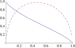
(b)  Divergence radius, $\chi(\mathscr{S}_{\circ}^{\gamma})$ (in bits, solid line), and peripheral information variance, $v_{\min}(\mathscr{S}_{\circ}^{\gamma})=v_{\max}(\mathscr{S}_{\circ}^{\gamma})$ (in bits², dashed line), as a function of $\gamma$.

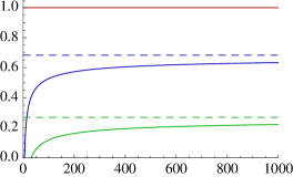
(c)  Second-Order approximation in (35) for $\frac{1}{n}\log M_{\textrm{sep}}^{*}\big{(}(\mathcal{E}_{\textrm{ad}}^{\gamma})^{\otimes n},\varepsilon\big{)}$ for $\varepsilon=1\%$, $\gamma\in\{0,\frac{1}{4},\frac{3}{4}\}$ (top to bottom) as a function of $n$. The dashed lines correspond to the asymptotic limit.

Figure 2: Geometry and second-order approximation for the amplitude damping channel.

Example 2.

The amplitude damping channel with magnitude $\gamma$ is given as

$$\mathcal{E}_{\textrm{ad}}^{\gamma}:\rho\mapsto\left(\begin{array}[]{cc}1&0\\ 0&\sqrt{1-\gamma}\end{array}\right)\rho\left(\begin{array}[]{cc}1&0\\ 0&\sqrt{1-\gamma}\end{array}\right)+\left(\begin{array}[]{cc}0&\sqrt{\gamma}\\ 0&0\end{array}\right)\rho\left(\begin{array}[]{cc}0&0\\ \sqrt{\gamma}&0\end{array}\right).$$ (44)

Its channel image, $\mathscr{S}_{\circ}^{\gamma}=\operatorname{im}(\mathcal{E}_{\textrm{ad}}^{\gamma})$, is displayed in Figure 2(a). In Fig. 2(b), the channel capacity and dispersion are evaluated numerically for different values of $\gamma$. The second-order approximation, i.e. the first two terms on the right-hand side of (35) are plotted as a function of $n$ in Figure 2(c).

It was already noted in (schumacher01, , Fig. 1) that it is necessary to consider non-orthogonal input states to achieve $\chi(\mathscr{S}_{\circ}^{\gamma})$ — in particular, $\mathcal{E}_{\textrm{ad}}^{\gamma}(|0\rangle\!\langle 0|)\notin\Gamma(\mathscr{S}_{\circ}^{\gamma})$ for general $\gamma\in(0,1)$.

This naturally leaves many open questions. Most intriguingly, it was recently shown that for entanglement-breaking and Hadamard channels, we have wilde13

$$\log M^{*}(\mathcal{E}^{n},\varepsilon)=n\,\chi(\mathscr{S}_{\circ})+O(\sqrt{n})$$ (45)

Thus, one could reasonably conjecture that a second-order approximation of the form (35) also holds for such channels (and not only image-additive channels). In particular, it would be interesting to see if the second-order term is again given by the peripheral information variance. The proof of the strong converse in wilde13 relies on the additivity of a suitable Rényi divergence radius lennert13 ; wilde13 of the channel image. However, it appears that their techniques are insufficient to derive a second-order expansion of the $\varepsilon$-hypothesis testing divergence radius.

IV Proofs: Quantum Divergence Radius

This section contains various lemmas which, combined, establish Theorem 2. Recall that $\mathscr{S}$ denotes the set of quantum states on a Hilbert space of dimension $d$, and $\mathscr{S}_{\circ}\subseteq\mathscr{S}$ is an arbitrary closed subset of $\mathscr{S}$, and thus also compact.

We will later show that the divergence center $\sigma^{*}(\mathscr{S}_{\circ})$, as defined in Theorem 2, is indeed a singleton, but at this point we have to be satisfied with the following statement.

Lemma 8.

The set $\sigma^{*}(\mathscr{S}_{\circ})$ is nonempty, convex and $\sigma\in\sigma^{*}(\mathscr{S}_{\circ})$ implies $\sigma\gg\rho$ for all $\rho\in\mathscr{S}_{\circ}$.

Proof.

Since $\mathscr{S}_{\circ}$ is compact, $\sup_{\rho\in\mathscr{S}_{\circ}}D(\rho\|\sigma)$ is finite if and only if $\sigma\gg\rho$ for all $\rho\in\mathscr{S}_{\circ}$. Moreover, since $\mathscr{S}$ is compact and the function $f:\sigma\mapsto\sup_{\rho\in\mathscr{S}_{\circ}}D(\rho\|\sigma)$ convex, the set of minima contains at least one element and is convex. ∎

In analogy to Theorem 2, we define the set of extremal points in $\mathscr{S}_{\circ}$ corresponding to the center $\sigma\in\sigma^{*}(\mathscr{S}_{\circ})$ as $\Gamma_{\sigma}(\mathscr{S}_{\circ}):=\operatorname*{\arg\max}_{\rho\in\mathscr{S}_{\circ}}D\big{(}\rho\big{\|}\sigma\big{)}$.

Proposition 9.

For every $\sigma\in\sigma^{*}(\mathscr{S}_{\circ})$, we have $\sigma\in\operatorname{conv}(\Gamma_{\sigma}(\mathscr{S}_{\circ}))$.

Proof.

Let us fix $\sigma\in\sigma^{*}(\mathscr{S}_{\circ})$ to simplify notation. We define

$$\Theta^{\nu}:=\big{\{}\rho\in\mathscr{S}_{\circ}\,\big{|}\,D(\rho\|\sigma)\geq\chi(\mathscr{S}_{\circ})-\nu\big{\}}.$$ (46)

and its complement $\bar{\Theta}^{\nu}:=\mathscr{S}_{\circ}\setminus\Theta^{\nu}$ for any $\nu\geq 0$. We first observe that $\Theta^{\nu}\subseteq\mathscr{S}_{\circ}$ is closed since $D(\cdot\|\sigma)$ is continuous and $\mathscr{S}_{\circ}$ is closed itself. Thus, both $\Theta^{\nu}$ and $\operatorname{conv}(\Theta^{\nu})$ are compact. Moreover, we clearly have $\bigcap_{\nu>0}\Theta^{\nu}=\Theta^{0}=\Gamma_{\sigma}(\mathscr{S}_{\circ})$.

For the sake of contradiction, let us now assume that $\sigma\notin\operatorname{conv}(\Theta^{\nu})$ for some fixed $\nu>0$. We employ the following lemma (also known as the Pythagorean theorem for relative entropy).

Lemma 10.

(ohya97, , Lem. 3.3) Let $\mathscr{S}_{\circ}\subseteq\mathscr{S}$ be compact convex and let $\sigma\in\mathscr{S}$. Then, $\tau:=\operatorname*{\arg\min}_{\tau\in\mathscr{S}_{\circ}}D(\tau\|\sigma)$ is unique. Moreover, for all $\rho\in\mathscr{S}_{\circ}$, we have

$$D(\rho\|\sigma)\geq D(\rho\|\tau)+D(\tau\|\sigma).$$ (47)

This establishes that there exists a unique state $\tau\in\operatorname{conv}(\Theta^{\nu})$ that minimizes $D(\tau\|\sigma)$. Furthermore, $D(\rho\|\sigma)>D(\rho\|\tau)$ for all $\rho\in\Theta^{\nu}$. Consequently, using the parametrization $\tau^{\lambda}:=\lambda\tau+(1-\lambda)\sigma$ and the convexity of $D(\rho\|\cdot)$, we find

$$D(\rho\|\tau^{\lambda})\leq\lambda D(\rho\|\tau)+(1-\lambda)D(\rho\|\sigma)<D(\rho\|\sigma)\qquad\forall\lambda\in(0,1).$$ (48)

Hence, $D(\rho\|\tau^{\lambda})<D(\rho\|\sigma)$ for all $\rho\in\Theta^{\nu}$ and for all $\lambda\in(0,1)$.

Furthermore, recall that $D(\rho\|\sigma)$ is bounded away from $\chi(\mathscr{S}_{\circ})$ for all $\rho\in\bar{\Theta^{\nu}}$ by definition. Due to the continuity of $D(\rho\|\cdot)$, we thus find that for sufficiently small $\lambda>0$,

$$D\big{(}\rho\big{\|}\tau^{\lambda}\big{)}<\chi(\mathscr{S}_{\circ})\qquad\forall\rho\in\mathscr{S}_{\circ}.$$ (49)

However, this implies that $\sigma\notin\sigma^{*}(\mathscr{S}_{\circ})$ and thus leads to a contradiction.

Hence, we conclude that $\sigma\in\operatorname{conv}(\Theta^{\nu})$ and since this holds for all $\nu>0$, we find $\sigma\in\bigcap_{\nu>0}\operatorname{conv}(\Theta^{\nu})$. The statement then follows by the following lemma proven in Appendix A.

Lemma 11.

Let $\Theta_{1}\supseteq\Theta_{2}\supseteq\ldots$ be a sequence of compact sets in a finite-dimensional vector space. Then,

$$\bigcap_{n\in\mathbb{N}}\operatorname{conv}(\Theta_{n})=\operatorname{conv}(\Theta_{\infty})\qquad\textrm{whenever}\qquad\Theta_{\infty}:=\bigcap_{n\in\mathbb{N}}\Theta_{n}\neq\emptyset.$$ (50)

This establishes that $\bigcap_{\nu>0}\operatorname{conv}(\Theta^{\nu})=\operatorname{conv}(\Theta^{0})$ and concludes the proof. ∎

The fact that $\sigma\in\sigma^{*}(\mathscr{S}_{\circ})\implies\sigma\in\operatorname{conv}(\Gamma_{\sigma}(\mathscr{S}_{\circ}))$, first established here, is crucial since it allows the following construction:

Due to Caratheodory’s theorem, we may decompose $\sigma$ into a convex combination of (at most $d^{2}$) peripheral states, namely we may write

$$\sigma=\sum_{\rho\in\mathscr{X}_{\circ}}P(\rho)\,\rho,\qquad\textrm{where}\quad\mathscr{X}_{\circ}\subseteq\Gamma_{\sigma}(\mathscr{S}_{\circ}),\ |\mathscr{X}_{\circ}|\leq d^{2}\quad\textrm{and}\quad P\in\mathcal{P}(\mathscr{X}_{\circ}).$$ (51)

Using this decomposition and the fact that $D(\rho\|\sigma)=\chi(\mathscr{S}_{\circ})$ for all $\rho\in\mathscr{X}_{\circ}$, we find

$$\chi(\mathscr{S}_{\circ})=\sum_{\rho\in\mathscr{X}_{\circ}}P(\rho)\,D(\rho\|\sigma)=H(\sigma)-\sum_{\rho\in\mathscr{X}_{\circ}}P(\rho)\,H(\rho)\,.$$ (52)

The uniqueness of $\sigma^{*}(\mathscr{S}_{\circ})$ now follows from a standard argument (see, e.g., (gallager68, , Sec. 4.5)) and using the strict concavity of $H$.

Lemma 12.

The set $\sigma^{*}(\mathscr{S}_{\circ})$ contains exactly one state.

Proof.

We have already established that $\sigma^{*}(\mathscr{S}_{\circ})$ is nonempty and convex in Lemma 8. Assume for the sake of contradiction that $\sigma_{0},\sigma_{1}\in\sigma^{*}(\mathscr{S}_{\circ})$ with $\sigma_{0}\neq\sigma_{1}$. Consequently, $\sigma_{\lambda}:=\lambda\sigma_{1}+(1-\lambda)\sigma_{0}$ is in $\sigma^{*}(\mathscr{S}_{\circ})$ for all $\lambda\in[0,1]$. Following (51), we may write

$$\sigma_{\lambda}=\sum_{\rho\in\mathscr{X}_{\circ}^{\prime}}P_{\lambda}(\rho)\,\rho,\qquad\textrm{where}\quad\mathscr{X}_{\circ}^{\prime}\subseteq\Gamma_{\sigma_{0}}(\mathscr{S}_{\circ})\cup\Gamma_{\sigma_{1}}(\mathscr{S}_{\circ}),\ |\mathscr{X}_{\circ}^{\prime}|\leq 2d^{2}\,.$$ (53)

and $P_{\lambda}(\rho)=\lambda P_{1}(\rho)+(1-\lambda)P_{0}(\rho)$ for $P_{\lambda}\in\mathcal{P}(\mathscr{X}_{\circ}^{\prime})$ . Then, due to (52), we have

$$\chi(\mathscr{S}_{\circ}) =H(\sigma_{0})-\sum_{\rho\in\mathscr{X}_{\circ}^{\prime}}P_{0}(\rho)H(\rho)=H(\sigma_{1})-\sum_{\rho\in\mathscr{X}_{\circ}^{\prime}}P_{1}(\rho)H(\rho).$$ (54)

Hence, using the strict concavity of $H(\cdot)$, we find

$$\chi(\mathscr{S}_{\circ}) =\lambda H(\sigma_{1})+(1-\lambda)H(\sigma_{0})-\sum_{\rho\in\mathscr{X}_{\circ}^{\prime}}P_{\lambda}(\rho)\,H(\rho)$$ (55)

$$<H(\sigma_{\lambda})-\sum_{\rho\in\mathscr{X}_{\circ}^{\prime}}P_{\lambda}(\rho)\,H(\rho)$$ (56)

$$=\sum_{\rho\in\mathscr{X}_{\circ}^{\prime}}P_{\lambda}(\rho)\,D(\rho\|\sigma_{\lambda}).$$ (57)

Finally, the fact that $D(\rho\|\sigma_{\lambda})\leq\sup_{\rho\in\mathscr{S}_{\circ}}D(\rho\|\sigma_{\lambda})=\chi(\mathscr{S}_{\circ})$ since $\sigma_{\lambda}\in\sigma^{*}(\mathscr{S}_{\circ})$ yields the desired contradiction. ∎

The previous lemma justifies writing $\Gamma(\mathscr{S}_{\circ})$ in Theorem 2, i.e. $\Gamma_{\sigma}(\mathscr{S}_{\circ})$ does not depend on $\sigma$. We will thus drop the subscript $\sigma$ in $\Gamma_{\sigma}$ hereafter.

For any $\mathbb{P}\in\mathcal{P}(\mathscr{S})$ and $\sigma\in\mathscr{S}$, let us introduce the notation

$$I(\mathbb{P}|\sigma):=\int\textnormal{d}\mathbb{P}(\rho)\,D(\rho\big{\|}\sigma)\quad\textrm{and}\quad I(\mathbb{P}):=I\Big{(}\mathbb{P}\Big{|}\rho^{(\mathbb{P})}\Big{)}$$ (58)

in analogy with the conditional mutual information.

Lemma 13.

We have $\chi(\mathscr{S}_{\circ})=\sup_{\mathbb{P}\in\mathcal{P}(\mathscr{S}_{\circ})}I(\mathbb{P})$. The supremum is achieved by a discrete probability measure with support on at most $d^{2}$ points in $\Gamma(\mathscr{S}_{\circ})$.

Proof.

First, note that for every $\mathbb{P}\in\mathcal{P}(\mathscr{S})$ we have $I(\mathbb{P})=\min_{\sigma\in\mathscr{S}}I(\mathbb{P}|\sigma)$ due to the positive-definiteness of $D(\cdot\|\cdot)$. Now, Sion’s minimax theorem sion58 yields

$$\sup_{\mathbb{P}\in\mathcal{P}(\mathscr{S}_{\circ})}\min_{\sigma\in\mathscr{S}}I(\mathbb{P}|\sigma)=\min_{\sigma\in\mathscr{S}}\sup_{\mathbb{P}\in\mathcal{P}(\mathscr{S}_{\circ})}I(\mathbb{P}|\sigma)$$ (59)

Indeed, it is easy to verify that $I(\mathbb{P}|\sigma)$ is convex in $\sigma$ and linear in $\mathbb{P}$. Moreover, $\mathscr{S}$ is compact convex and $\mathcal{P}(\mathscr{S}_{\circ})$ is convex, as required. Finally, the supremum over distributions on the right-hand side of (59) can be replaced by a supremum over Dirac measures on $\mathscr{S}_{\circ}$ without loss of generality. This establishes

$$\sup_{\mathbb{P}\in\mathcal{P}(\mathscr{S}_{\circ})}\int\textnormal{d}\mathbb{P}(\rho)\,D(\rho\big{\|}\rho^{(\mathbb{P})})=\min_{\sigma\in\mathscr{S}}\sup_{\rho\in\mathscr{S}_{\circ}}D(\rho\|\sigma).$$ (60)

The second statement follows immediately due to the construction given in Eq. (51) and (52). ∎

We are now ready to summarize the proof of Theorem 2.

Proof of Theorem 2.

Property 1 follows from Lemmas 8 and 12. Property 2 is a trivial consequence of Property 1 and the definition of $\Gamma$. Property 3 is implied by Proposition 9 whereas Property 4 is established in Lemma 13. Finally, Property 5 is established as follows:

Clearly, every $\mathbb{P}\in\Pi(\mathscr{S}_{\circ})$ achieves the supremum in (18), $\chi(\mathscr{S}_{\circ})$, by definition of $\Gamma(\mathscr{S}_{\circ})$. Conversely, let us assume that there exists a distribution $\mathbb{P}\in\mathcal{P}$ that achieves $\chi(\mathscr{S}_{\circ})$. Then, $\rho^{(\mathbb{P})}=\sigma^{*}(\mathscr{S}_{\circ})$ by the argument in Lemmas 12 and 13. Moreover, $\mathbb{P}[\Gamma(\mathscr{S}_{\circ})]=1$ is necessary due to the definition of $\Gamma$. ∎

V Proofs: Second-Order Approximation

The direct part of the proof of Theorem 4 is presented in Section V.1. We split the proof of the converse part of Theorem 4 into several parts. First, Section V.2 provides a proof of our one-shot converse bound in Proposition 5. Then, Section V.3 introduces some non-asymptotic bounds on the $\varepsilon$-hypothesis testing divergence for product states that are essential for our asymptotic analysis. As a warm-up, Section V.4 shows the strong converse property for c-q channels using these techniques. The converse part of Theorem 4 is then established in Section V.5, and an improved third-order bound for discrete classical-quantum channels is given in V.6.

V.1 Proof of Direct Part of Thoerem 4

We base our result on the following straightforward generalization of the one-shot bounds by Hayashi and Nagaoka hayashi03 in the form of Wang and Renner wang10 (see also datta11a ; renes10-2 ; dupuisszehr12 for recent one-shot achievability bounds for c-q channels).

Proposition 14.

(wang10, , Thm. 1) Let $\varepsilon\in(0,1)$, $\eta\in(0,\varepsilon)$, and let $\mathscr{X}_{\circ}\subseteq\operatorname{im}(\mathcal{W})$ be discrete. Then,

$$\log M^{*}(\mathcal{W},\varepsilon)\geq \sup_{P\in\mathcal{P}(\mathscr{X}_{\circ})}D_{h}^{\varepsilon-\eta}\Bigg{(}\bigoplus_{\rho\in\mathscr{X}_{\circ}}P(\rho)\rho\,\Bigg{\|}\bigoplus_{\rho\in\mathscr{X}_{\circ}}P(\rho)\rho^{(P)}\Bigg{)}-\log\frac{4\varepsilon(1-\varepsilon+\eta)}{\eta^{2}}.$$ (61)

We can include the closure of $\operatorname{im}(\mathcal{W})$ due to the continuity of the above expression when the set $\mathscr{X}_{\circ}$ is varied by replacing an element with one that is close in $(\mathscr{S},\delta_{textrm{tr}})$. Thus, our bound reads

$$\log M^{*}(\mathcal{W},\varepsilon)\geq\sup_{\mathscr{X}_{\circ}\subseteq\overline{\operatorname{im}(\mathcal{W})}}\sup_{P\in\mathcal{P}(\mathscr{X}_{\circ})}D_{h}^{\varepsilon-\eta}\Big{(}\omega^{(P)}\Big{\|}\tau^{(P)}\otimes\rho^{(P)}\Big{)}-\log\frac{4\varepsilon(1-\varepsilon+\eta)}{\eta^{2}},$$ (62)

where $\mathscr{X}_{\circ}$ is discrete and we introduced the shorthands $\omega^{(P)}:=\bigoplus_{\rho\in\mathscr{X}_{\circ}}P(\rho)\rho$ and $\tau^{(P)}:=\bigoplus_{\rho\in\mathscr{X}_{\circ}}P(\rho)$. The similarity of the above expression with the asymptotic expression in (18) is evident once (18) is specialized to the discrete case as well.

The restriction to finite subsets of $\mathscr{S}_{\circ}$ is unproblematic in light of Lemma 3. Let us then proceed to prove the lower bound in Theorem 4, which we restate in a slightly stronger form here.

Direct Part of Theorem 4.

Let $\varepsilon\in(0,1)$ and let $\mathcal{W}$ be a c-q channel. Set $\mathscr{S}_{\circ}:=\overline{\operatorname{im}(\mathcal{W})}$. Then,

$$\log M^{*}(\mathcal{W}^{n},\varepsilon)\geq n\,\chi(\mathscr{S}_{\circ})+\sqrt{n\,v_{\varepsilon}(\mathscr{S}_{\circ})}\,\Phi^{-1}(\varepsilon)+O(\log n).$$ (63)

Proof.

First, let us apply (62) to the $n$-fold repetition of the channel $\mathcal{W}$. Fixing any discrete set $\mathscr{X}_{\circ}\subseteq\mathscr{S}_{\circ}$ and $P\in\mathcal{P}(\mathscr{X}_{\circ})$, we first confirm that

$$\log M^{*}(\mathcal{W}^{n},\varepsilon)\geq D_{h}^{\varepsilon-\eta}\Big{(}\big{(}\omega^{(P)}\big{)}^{\otimes n}\Big{\|}\big{(}\tau^{(P)}\otimes\rho^{(P)}\big{)}^{\otimes n}\Big{)}-\log\frac{4\varepsilon(1-\varepsilon+\eta)}{\eta^{2}}$$ (64)

Note that we applied (62) using the set $\mathscr{X}_{\circ}^{\otimes n}\subseteq\overline{\operatorname{im}(\mathcal{W})}^{\otimes n}=\overline{\operatorname{im}(\mathcal{W})^{\otimes n}}$ and the $n$-fold product distribution $P^{\times n}$. By Lemma 3 there exists a probability mass function (let it be our choice of $P$) with support on $\Gamma(\mathscr{S}_{\circ})$ (let the support set be our choice of $\mathscr{X}_{\circ}$) such that

$$\rho^{(P)}=\sigma,\quad\sum_{\rho\in\mathscr{X}_{\circ}}P(\rho)\,D(\rho\|\sigma)=\chi(\mathscr{S}_{\circ}),\quad\textrm{and}\quad\sum_{\rho\in\mathscr{X}_{\circ}}P(\rho)\,V(\rho\|\sigma)=v_{\varepsilon}(\mathscr{S}_{\circ}),$$ (65)

where we set $\sigma=\sigma^{*}(\mathscr{S}_{\circ})$. Now, we can verify that

$$\sum_{\rho\in\mathscr{X}_{\circ}}P(\rho)\,D\big{(}\rho\big{\|}\rho^{(P)}\big{)}=D\Bigg{(}\bigoplus_{\rho\in\mathscr{X}_{\circ}}P(\rho)\rho\,\Bigg{\|}\bigoplus_{\rho\in\mathscr{X}_{\circ}}P(\rho)\rho^{(P)}\Bigg{)},$$ (66)

and, the following simple generalization of (polyanskiy10, , Lm. 62) proved in Appendix D holds.

Lemma 15.

For any probability mass function $P\in\Pi(\mathscr{S}_{\circ})$, we have

$$\sum_{\rho\in\mathscr{X}_{\circ}}P(\rho)\,V\big{(}\rho\big{\|}\rho^{(P)}\big{)}=V\Bigg{(}\bigoplus_{\rho\in\mathscr{X}_{\circ}}P(\rho)\rho\,\Bigg{\|}\bigoplus_{\rho\in\mathscr{X}_{\circ}}P(\rho)\rho^{(P)}\Bigg{)}.$$ (67)

As such, we are left to evaluate the asymptotics of $D_{h}^{\varepsilon-\eta}$ for identical product states. Let us set $\varepsilon_{n}:=\varepsilon-\eta$ with $\eta=1/{\sqrt{n}}$. First, consider the case where $v_{\varepsilon}(\mathscr{S}_{\circ})>0$. The second assertion in Proposition 16 (i.e. the bound in (80)) specialized to i.i.d. states, establishes that

$$D_{h}^{\varepsilon-\eta}\Big{(}\big{(}\omega^{(P)}\big{)}^{\otimes n}\Big{\|}\big{(}\tau^{(P)}\otimes\rho^{(P)}\big{)}^{\otimes n}\Big{)}$$ (68)

$$\qquad\qquad\geq nD\big{(}\omega^{(P)}\big{\|}\tau^{(P)}\otimes\rho^{(P)}\big{)}+\sqrt{nV\big{(}\omega^{(P)}\big{\|}\tau^{(P)}\otimes\rho^{(P)}\big{)}}\,\Phi^{-1}(\varepsilon)-L_{2}\log n$$ (69)

$$\qquad\qquad=n\chi(\mathscr{S}_{\circ})+\sqrt{n\,v_{\varepsilon}(\mathscr{S}_{\circ})}\,\Phi^{-1}(\varepsilon)-L_{2}\log n\,.$$ (70)

for all $n\geq N_{2}$ and some constants $L_{2}$ and $N_{2}(\varepsilon,\mathscr{S}_{\circ})$. In the last step we employed (66), Lemma 15 and (65). Moreover, the last summand in (64) is of the form $O(\log n)$ and we are done.

The proof for the case $v_{\varepsilon}(\mathscr{S}_{\circ})=0$ proceeds similarly but employs the first bound in Eq. (79) in Proposition 16 instead. This yields

$$D_{h}^{\varepsilon-\eta}\Big{(}\big{(}\omega^{(P)}\big{)}^{\otimes n}\Big{\|}\big{(}\tau^{(P)}\otimes\rho^{(P)}\big{)}^{\otimes n}\Big{)}\geq nD\big{(}\omega^{(P)}\big{\|}\tau^{(P)}\otimes\rho^{(P)}\big{)}-L_{1}\log n.$$ (71)

for all $n\geq N_{1}$ and some constants $L_{1}$ and $N_{1}(\varepsilon-\eta,\mathscr{S}_{\circ})$. The rest of the proof then proceeds analogously to the discussion above. ∎

V.2 Proof of Proposition 5

Let us recall the statement of Proposition 5. For $\varepsilon\in(0,1)$ and $\mu\in(0,1-\varepsilon)$, we want that

$$\log M^{*}(\mathcal{W},\varepsilon)\leq\chi_{h}^{\varepsilon+\mu}\Big{(}\overline{\operatorname{im}(\mathcal{W})}\Big{)}+\log\frac{\varepsilon+\mu}{\mu(1-\varepsilon-\mu)}.$$ (72)

Proof of Proposition 5.

Let $\mathcal{C}=\{\mathscr{M},e,\mathcal{D}\}$ be a code with $p_{\textrm{err}}(\mathcal{C},\mathcal{W})\leq\varepsilon$ given by codewords $x_{m}=e(m)\in\mathscr{X}$ and a decoder $\mathcal{D}=\{Q_{m}\}_{m\in\mathscr{M}}$. By assumption, we thus have $\frac{1}{|\mathscr{M}|}\sum_{m\in\mathscr{M}}\operatorname{tr}(Q_{m}\mathcal{W}(x_{m}))\geq 1-\varepsilon$. For an arbitrary but fixed $\sigma\in\mathscr{S}$, we define the set

$$\mathcal{K}:=\big{\{}m\in\mathscr{M}\,\big{|}\operatorname{tr}\big{(}Q_{m}\mathcal{W}(x_{m})\big{)}\geq 1-\varepsilon-\mu\big{\}},\quad\textrm{and}\quad m^{*}:=\operatorname*{\arg\min}_{m\in\mathcal{K}}\ \operatorname{tr}(Q_{m}\sigma).$$ (73)

By definition of this set, we have

$$1-\varepsilon\leq\frac{1}{|\mathscr{M}|}\sum_{m\in\mathscr{M}}\operatorname{tr}(Q_{m}\mathcal{W}(x_{m})) =\frac{1}{|\mathscr{M}|}\sum_{m\in\mathcal{K}}\operatorname{tr}(Q_{m}\mathcal{W}(x_{m}))+\frac{1}{|\mathscr{M}|}\sum_{m\in\mathscr{M}\setminus\mathcal{K}}\operatorname{tr}(Q_{m}\mathcal{W}(x_{m}))$$ (74)

$$<\frac{|\mathcal{K}|}{|\mathscr{M}|}+\frac{|\mathscr{M}|-|\mathcal{K}|}{|\mathscr{M}|}(1-\varepsilon-\mu)$$ (75)

Hence, $|\mathcal{K}|>|\mathscr{M}|\frac{\mu}{\varepsilon+\mu}$. Moreover, we have

$$1=\operatorname{tr}(\sigma)=\sum_{m\in\mathscr{M}}\operatorname{tr}(Q_{m}\sigma)\geq|\mathcal{K}|\operatorname{tr}(Q_{{m^{*}}}\sigma)>|\mathscr{M}|\frac{\mu}{\varepsilon+\mu}\operatorname{tr}(Q_{{m^{*}}}\sigma).$$ (76)

By definition of the $\varepsilon$-hypothesis testing divergence we find

$$D_{h}^{\varepsilon+\mu}(\mathcal{W}(x_{m^{*}})\|\sigma)\geq-\log\frac{\operatorname{tr}(Q_{{m^{*}}}\sigma)}{1-\varepsilon-\mu}>\log|\mathscr{M}|-\log\frac{\varepsilon+\mu}{\mu(1-\varepsilon-\mu)}.$$ (77)

Thus, in particular we have

$$\sup_{\rho\in\,\overline{\operatorname{im}(\mathcal{W})}}\,D_{h}^{\varepsilon+\mu}(\rho\|\sigma)>\log|\mathscr{M}|-\log\frac{\varepsilon+\mu}{\mu(1-\varepsilon-\mu)}$$ (78)

Finally, Eq. (72) follows by observing that the above bound holds for all $\sigma\in\mathscr{S}$. ∎

V.3 Non-Asymptotic Bounds on the Hypothesis-Testing Divergence

Some of the main ingredients of our asymptotic analysis in the converse part of the proof of Theorem 4 are the following non-asymptotic bounds on the $\varepsilon$-hypothesis testing divergence evaluated for product states. Before we state the bounds, recall that $I(\mathbb{P}|\sigma)=\int\textnormal{d}\mathbb{P}(\rho)\,D(\rho\|\sigma)$ and define $V(\mathbb{P}|\sigma):=\int\textnormal{d}\mathbb{P}(\rho)\,V(\rho\|\sigma)$ analogously for any $\mathbb{P}\in\mathcal{P}(\mathscr{S})$ and $\sigma\in\mathscr{S}$. Moreover, given a sequence of states $\rho^{n}=\bigotimes_{i=1}^{n}\rho_{i}$, we denote by $P_{\rho^{n}}(\rho):=\frac{1}{n}\sum_{i=1}^{n}1\{\rho=\rho_{i}\}$ the empirical distribution of $\rho^{n}$.

Proposition 16.

Let $\varepsilon\in(0,1)$, $\mathscr{S}_{\circ}\subseteq\mathscr{S}$ and $\lambda_{0}>0$. Let $\{\varepsilon_{n}\}_{n=1}^{\infty}$ be any sequence satisfying $|\varepsilon_{n}-\varepsilon|\leq 1/\sqrt{n}$ for all $n$ and set $\varepsilon^{*}:=\min\{\varepsilon,1-\varepsilon\}$. Then, there exist constants $N_{1}(\varepsilon,\mathscr{S}_{\circ},\lambda_{0})$ and $K_{1}(\varepsilon,\mathscr{S}_{\circ},\lambda_{0})$ and $L_{1}$ such that the following holds. For every $n\geq N_{1}$, every $\sigma\in\mathscr{S}$ with $\lambda_{\min}(\sigma)\geq\lambda_{0}$ and every sequence $\rho^{n}=\bigotimes_{i=1}^{n}\rho_{i}$, $\rho_{i}\in\mathscr{S}_{\circ}$, we have

$$\Big{|}\,D_{h}^{\varepsilon_{n}}\big{(}\rho^{n}\big{\|}\,\sigma^{\otimes n}\big{)}-nI\big{(}P_{\rho^{n}}\big{|}\sigma\big{)}\Big{|}\leq\sqrt{\frac{nV(P_{\rho^{n}}|\sigma)}{\varepsilon^{*}}}+L_{1}\log n\leq K_{1}\sqrt{n}\,.$$ (79)

Further let $\xi>0$ and fix $\sigma\in\mathscr{S}$ with $\lambda_{\min}(\sigma)>0$. Then, there exist constants $N_{2}(\varepsilon,\mathscr{S}_{\circ},\sigma,\xi)$ and $L_{2}$ such that the following holds. For every $n\geq N_{2}$ and every sequence $\rho^{n}=\bigotimes_{i=1}^{n}\rho_{i}$, $\rho_{i}\in\mathscr{S}_{\circ}$ satisfying $V(P_{\rho^{n}}|\sigma)\geq\xi$, we have

$$\Big{|}\,D_{h}^{\varepsilon_{n}}\big{(}\rho^{n}\big{\|}\,\sigma^{\otimes n}\big{)}-nI\big{(}P_{\rho^{n}}\big{|}\sigma\big{)}-\sqrt{nV\big{(}P_{\rho^{n}}\big{|}\sigma\big{)}}\,\Phi^{-1}(\varepsilon)\Big{|}\leq L_{2}\log n.$$ (80)

Finally, if $\sigma=\rho^{(P_{\rho^{n}})}$ in (80), then the statement holds for $n\geq N_{3}(\varepsilon,\mathscr{S}_{\circ},\xi)$ independent of $\sigma$.

In the asymptotic limit as $n\to\infty$, all inequalities imply the seminal quantum Stein’s lemma hiai91 and its strong converse ogawa00 when the sequence is chosen i.i.d. The proof is based on the techniques of li12 ; tomamichel12 and presented in Appendix B. It is crucial for our application that $L_{1},L_{2},K_{1},N_{1},N_{2}$ and $N_{3}$ are uniform over $\sigma$ and sequences $\rho^{n}$ satisfying the constraints. This is nontrivial and requires arguments beyond those in li12 ; tomamichel12 which only treat the i.i.d. case.

V.4 Asymptotics of the $\varepsilon$-Hypothesis Testing Divergence Radius: First-Order

As a warm-up, we use our techniques to provide a simple proof of the strong converse property of general classical-quantum channels. The strong converse is evidently a corollary of Proposition 5 and the following result.

Proposition 17.

Let $\varepsilon\in(0,1)$ and $\mathscr{S}_{\circ}\subseteq\mathscr{S}$ closed. Let $\{\varepsilon_{n}\}_{n=1}^{\infty}$ be any sequence satisfying $|\varepsilon_{n}-\varepsilon|\leq 1/\sqrt{n}$ for all $n$. Then,

$$\chi_{h}^{\varepsilon_{n}}\big{(}\mathscr{S}_{\circ}^{\otimes n}\big{)}\leq n\,\chi(\mathscr{S}_{\circ})+O(\sqrt{n}).$$ (81)

Note that Winter winterthesis and Ogawa-Nagaoka ogawa99 first showed the strong converse for classical-quantum channels for the generality we consider here.

Proof.

By definition of the $\varepsilon$-hypothesis testing divergence radius, we have

$$\chi_{h}^{\varepsilon_{n}}\big{(}\mathscr{S}_{\circ}^{\otimes n}\big{)}\leq\sup_{\rho^{n}\in\mathscr{S}_{\circ}^{\otimes n}}D_{h}^{\varepsilon_{n}}\big{(}\rho^{n}\,\big{\|}\,\sigma^{\otimes n}\big{)},$$ (82)

where we chose an $n$-fold product of the divergence center, $\sigma=\sigma^{*}(\mathscr{S}_{\circ})\in\mathscr{S}$, as the output state. The states $\rho^{n}$ are of the form $\rho^{n}=\bigotimes_{i=1}^{n}\rho_{i}$. For a fixed and arbitrary $\rho^{n}$, we define the set $\mathscr{S}_{\circ}^{n}:=\{\rho_{i}\}_{i=1}^{n}\subseteq\mathscr{S}_{\circ}$ and the empirical distribution $P_{\rho^{n}}\in\mathcal{P}\big{(}\mathscr{S}_{\circ}^{n}\big{)}$ given by $P_{\rho^{n}}(\rho)=\frac{1}{n}\sum_{i=1}^{n}1\{\rho=\rho_{i}\}$.

We then use (79) in Proposition 16 to assert that

$$D_{h}^{\varepsilon_{n}}\big{(}\rho^{n}\,\big{\|}\,\sigma^{\otimes n}\big{)}\leq nI(P_{\rho^{n}}|\sigma)+K_{1}\sqrt{n}$$ (83)

for sufficiently large $n\geq N_{1}$. Here, we used that $\lambda_{\min}(\sigma)>0$ and recall that $I(\mathbb{P}|\sigma)$ is defined as $I(\mathbb{P}|\sigma)=\int\textnormal{d}\mathbb{P}(\rho)\,D(\rho\|\sigma)$. Therefore, Theorem 2 ensures that $D(\rho\|\sigma)\leq\chi(\mathscr{S}_{\circ})$ for all $\rho\in\mathscr{S}_{o}$ and we have established that

$$\chi_{h}^{\varepsilon_{n}}\big{(}\mathscr{S}_{\circ}^{\otimes n}\big{)}\leq\sup_{\rho^{n}\in\mathscr{S}_{\circ}^{\otimes n}}nI(P_{\rho^{n}}|\sigma)+K_{1}\sqrt{n}\leq n\chi(\mathscr{S}_{\circ})+K_{1}\sqrt{n}.\qed$$ (84)

V.5 Asymptotics of the $\varepsilon$-Hypothesis Testing Divergence Radius: Second-Order

In view of Proposition 5 and the discussion in the previous section, we therefore want to find a second-order upper bound on $\chi_{h}^{\varepsilon}\big{(}\mathscr{S}_{\circ}^{\otimes n}\big{)}=\min_{\sigma^{n}\in\mathscr{S}^{n}}\sup_{\rho^{n}\in\mathscr{S}_{\circ}^{\otimes n}}D_{h}^{\varepsilon}\big{(}\rho^{n}\|\sigma^{n}\big{)}$. The following results constitute the main technical contribution of this paper.

V.5.1 An Appropriate Choice of $\sigma^{n}$

The proof of the strong converse in Propositon 17 hinges on choosing $\sigma^{n}$ as the $n$-fold product of the divergence center and then taking advantage of the fact that $D(\rho\|\sigma)\leq\chi(\mathscr{S}_{\circ})$ for all $\rho\in\mathscr{S}_{\circ}$. This will not be sufficient if we want to pin down the exact second-order term proportional to $\sqrt{n}$.

Before we commence, we thus introduce an appropriate choice of auxiliary state $\sigma^{n}$. To construct it, we require the following auxiliary result whose proof is provided in Appendix C. This establishes that there exists a $\gamma$-net on $\mathscr{S}_{\circ}$ whose cardinality can be bounded appropriately.

Lemma 18.

For every $\gamma\in(0,1)$, there exists a set of states $\mathscr{G}^{\gamma}\subseteq\mathscr{S}$ of size

$$|\mathscr{G}^{\gamma}|\leq\left(\frac{5}{\gamma}\right)^{2d^{2}}\left(\frac{2d}{\gamma}+2\right)^{d-1}$$ (85)

such that, for every $\rho\in\mathscr{S}$, there exists a state $\tau\in\mathscr{G}^{\gamma}$ satisfying the following:

$$\frac{1}{2}\|\rho-\tau\|_{1}\leq\gamma,\quad D(\rho\|\tau)\leq\gamma\cdot 4(2d+1),\quad\textrm{and}\quad\lambda_{\min}(\tau)\geq\frac{\gamma}{2d+\gamma}.$$ (86)

Now, for a $\gamma$ to be specified below, we choose the output state $\sigma^{n}\in\mathscr{S}^{n}$ as follows:

$$\sigma^{n}:=\frac{1}{2}\sigma^{\otimes n}+\frac{1}{2|\mathscr{G}^{\gamma}|}\sum_{\tau\in\mathscr{G}^{\gamma}}\tau^{\otimes n},\qquad\textrm{where}\quad\sigma=\sigma^{*}(\mathscr{S}_{\circ}).$$ (87)

Note that $\sigma^{n}$ is normalized and is, in fact, a convex combination of the $n$-fold tensor product of the divergence center and the $n$-fold tensor product of the elements of the net, of which there are only finitely many. With this choice of $\sigma^{n}$ we bound $D_{h}^{\varepsilon}\big{(}\rho^{n}\|\sigma^{n}\big{)}$ in the following.

V.5.2 Different Sequences of Inputs

We will also need to treat different types of state sequences separately. We keep $\mathscr{S}_{\circ}$ fixed for the following to simplify notation. Let us define $\Omega_{1}^{\nu},\Omega_{2}^{\nu}\subseteq\mathscr{S}_{\circ}^{\otimes n}$ for some $0<\nu\leq 1$, which describe sets of state sequences of length $n$ that are close to achieving the first-order fundamental limit. (We omit the dependence on $n$ in our notation here.) The first set ensures that the states are close to $\Gamma(\mathscr{S}_{\circ})$, and is defined as

$$\Omega_{1}^{\nu}:=\Bigg{\{}\rho^{n}\in\mathscr{S}_{\circ}^{\otimes n}\ \Bigg{|}\ \frac{1}{n}\sum_{i=1}^{n}\underbrace{\min_{\tau\in\Gamma(\mathscr{S}_{\circ})}\frac{1}{2}\|\rho_{i}-\tau\|_{1}}_{=:\,\Delta(\rho_{i},\Gamma(\mathscr{S}_{\circ}))}\leq\nu\Bigg{\}}.$$ (88)

The second set ensures that the average state is close to the divergence center, and is defined as

$$\Omega_{2}^{\nu}:=\Bigg{\{}\rho^{n}\in\mathscr{S}_{\circ}^{\otimes n}\ \Bigg{|}\ \frac{1}{2}\bigg{\|}\frac{1}{n}\sum_{i=1}^{n}\rho_{i}-\sigma^{*}(\mathscr{S}_{\circ})\bigg{\|}_{1}\leq\nu\Bigg{\}}.$$ (89)

The interesting, close to capacity-achieving sequences are those that are in $\Omega_{1}^{\nu}\cap\Omega_{2}^{\nu}$.

V.5.3 Dealing with Sub-Optimal Input Sequences

We first deal with sequences that are far from optimal in the sense prescribed above.

Proposition 19.

Let $\varepsilon\in(0,1)$, $\nu>0$ and $\mathscr{S}_{\circ}\subseteq\mathscr{S}$. Let $\{\varepsilon_{n}\}_{n=1}^{\infty}$ be any sequence satisfying $|\varepsilon_{n}-\varepsilon|\leq 1/\sqrt{n}$ for all $n$. Then, there exist constants $N_{0}(\varepsilon,\mathscr{S}_{\circ},\nu)$ and $\gamma_{0}(\mathscr{S}_{\circ},\nu)$ such that, for all $n\geq N_{0}$ and all $\rho^{n}\notin\Omega_{1}^{\nu}\cap\Omega_{2}^{\nu}$, we have

$$D_{h}^{\varepsilon_{n}}(\rho^{n}\|\sigma^{n})\leq n\,\chi(\mathscr{S}_{\circ})+\sqrt{n\,v_{\varepsilon}(\mathscr{S}_{\circ})}\,\Phi^{-1}(\varepsilon),$$ (90)

where $\sigma^{n}$ is defined as in (87) for a fixed $\gamma=\gamma_{0}$.

Proof.

The technique for bounding $D_{h}^{\varepsilon_{n}}\big{(}\rho^{n}\|\sigma^{n}\big{)}$ differs depending on the state sequence $\rho^{n}$. We consider two cases: (a) $\rho^{n}\notin\Omega_{1}^{\nu}$ and (b) $\rho^{n}\notin\Omega_{2}^{\nu}$ in the following subsections.

(a) Sequences $\rho^{n}\notin\Omega_{1}^{\nu}$:

Applying Property 3 of Lemma 1 to $D_{h}^{\varepsilon_{n}}(\rho^{n}\|\sigma^{n})$ with our choice of $\sigma^{n}$ in (87) and picking out the divergence center $\sigma^{\otimes n}$ yields an upper bound of the form

$$D_{h}^{\varepsilon_{n}}(\rho^{n}\|\sigma^{n}) \leq D_{h}^{\varepsilon_{n}}(\rho^{n}\|\sigma^{\otimes n}\big{)}+\log 2.$$ (91)

Furthermore, as in the proof of Proposition 17, we employ (79) in Proposition 16 to obtain

$$D_{h}^{\varepsilon_{n}}\big{(}\rho^{n}\big{\|}\sigma^{\otimes n}\big{)} \leq\sum_{i=1}^{n}D(\rho_{i}\|\sigma)+K_{1}\sqrt{n}\,,$$ (92)

for all $n\geq N_{1}$. (We absorbed the constant term $\log 2$ into the constant $K_{1}$ here for convinience.)

Now, we define $\hat{\chi}^{\nu}_{1}:=\sup_{\rho\in\mathscr{S}_{\circ}:\,\Delta(\rho,\Gamma)>\frac{\nu}{2}}D(\rho\|\sigma)<\chi(\mathscr{S}_{\circ})$ and employ the following lemma which is shown in Appendix D.

Lemma 20.

Let $\rho^{n}\in\mathscr{S}_{\circ}^{\otimes n}$ be fixed and let $\nu\in(0,1)$. If $\rho^{n}\notin\Omega_{1}^{\nu}$, then there exists a set $\Xi^{\nu}\subseteq[n]$ of cardinality $|\Xi^{\nu}|>n\frac{\nu}{2}$ such that, for all $i\in\Xi^{\nu}$, we have $\Delta(\rho_{i},\Gamma)>\frac{\nu}{2}$.

This leads us to bound

$$D_{h}^{\varepsilon_{n}}(\rho^{n}\|\sigma^{n})\leq\sum_{i\in\Xi^{\nu}}\hat{\chi}^{\nu}_{1}+\sum_{i\notin\Xi^{\nu}}\chi(\mathscr{S}_{\circ})+K_{1}\sqrt{n}\leq n\chi(\mathscr{S}_{\circ})-n(\chi(\mathscr{S}_{\circ})-\hat{\chi}^{\nu}_{1})\frac{\nu}{2}+K_{1}\sqrt{n}.$$ (93)

In particular, we have $D_{h}^{\varepsilon_{n}}(\rho^{n}\|\sigma^{n})\leq n\,\chi(\mathscr{S}_{\circ})+\sqrt{n\,v_{\varepsilon}(\mathscr{S}_{\circ})}\Phi^{-1}(\varepsilon)$ for sufficiently large $n\geq N$, where $N$ is appropriately chosen.

(b) Sequences $\rho^{n}\notin\Omega_{2}^{\nu}$:

For these sequences, we extract the state $\tau^{\otimes n}$ from the convex combination that defines $\sigma^{n}$ in (87), where $\tau$ is the state closest (in the relative entropy sense) to the average output state $\bar{\rho}=\rho^{(P_{\rho^{n}})}=\frac{1}{n}\sum_{i=1}^{n}\rho_{i}$ in $\mathscr{G}^{\gamma}$ and the constant $\gamma>0$ is to be chosen later. In other words, $\tau\in\operatorname*{\arg\min}_{\tau\in\mathscr{G}^{\gamma}}D(\bar{\rho}\|\tau)$. Thus, by Property 3 of Lemma 1, we have

$$D_{h}^{\varepsilon_{n}}(\rho^{n}\|\sigma^{n})\leq D_{h}^{\varepsilon_{n}}\big{(}\rho^{n}\big{\|}\tau^{\otimes n}\big{)}+\log|\mathscr{G}^{\gamma}|.$$ (94)

Then, by using (79) in Proposition 16 we find for all $\rho^{n}\notin\Omega_{2}^{\nu}$ that

$$D_{h}^{\varepsilon_{n}}\big{(}\rho^{n}\big{\|}\tau^{\otimes n}\big{)} \leq\sum_{i=1}^{n}D(\rho_{i}\|\tau)+K_{1}^{\prime}\sqrt{n}.$$ (95)

for $n\geq N_{1}^{\prime}$. Here, we take advantage of the fact that the minimum eigenvalue of $\tau$ satisfies $\lambda_{\min}(\tau)\geq\frac{\gamma}{2d+\gamma}$ such that the constants $K_{1}^{\prime}$ and $N_{1}^{\prime}$ can be chosen uniformly for all $\tau\in\mathscr{G}^{\gamma}$.

We continue to bound

$$D_{h}^{\varepsilon_{n}}\big{(}\rho^{n}\big{\|}\tau^{\otimes n}\big{)} \leq\sum_{i=1}^{n}D(\rho_{i}\|\bar{\rho})+\sum_{i=1}^{n}\operatorname{tr}\big{(}\rho_{i}(\log\bar{\rho}-\log\tau)\big{)}+K_{1}^{\prime}\sqrt{n}$$ (96)

$$=\sum_{i=1}^{n}D(\rho_{i}\|\bar{\rho})+nD(\bar{\rho}\|\tau)+K_{1}^{\prime}\sqrt{n}$$ (97)

$$\leq n\,I\Big{(}P_{\rho^{n}}\Big{|}\,\rho^{(P_{\rho^{n}})}\Big{)}+n\cdot 4\gamma(2d+1)+K_{1}^{\prime}\sqrt{n},$$ (98)

where the second inequality follows from the properties of the $\gamma$-net stated in Lemma 18 and on the last line we introduced the empirical distribution of $\rho^{n}$, defined as $P_{\rho^{n}}(\rho)=\frac{1}{n}\sum_{i=1}^{n}1\{\rho=\rho_{i}\}$.

Then, by Theorem 2 and the definition of $\Pi(\mathscr{S}_{\circ})$ and $\nu\in(0,1)$, we know that

$$\tilde{\chi}^{\nu}_{2}:=\sup\bigg{\{}I\Big{(}\mathbb{P}\Big{|}\rho^{(\mathbb{P})}\Big{)}\,\bigg{|}\,\mathbb{P}\in\mathcal{P}(\mathscr{S}_{\circ}):\,\frac{1}{2}\Big{\|}\rho^{(\mathbb{P})}-\sigma^{*}(\mathscr{S}_{\circ})\Big{\|}_{1}>\nu\bigg{\}}<\chi(\mathscr{S}_{\circ}).$$ (99)

Summarizing the above, we have

$$D_{h}^{\varepsilon_{n}}(\rho^{n}\|\sigma^{n})\leq n\chi(\mathscr{S}_{\circ})-n\big{(}\chi(\mathscr{S}_{\circ})-\tilde{\chi}^{\nu}_{2}-4\gamma(2d+1)\big{)}+K_{1}^{\prime}\sqrt{n}+\log|\mathscr{G}^{\gamma}|.$$ (100)

By choosing $\gamma=\gamma_{0}(\nu,\mathscr{S}_{\circ})$ small enough such that $\chi(\mathscr{S}_{\circ})-\tilde{\chi}^{\nu}_{2}-4\gamma(2d+1)>0$, we find that $D_{h}^{\varepsilon_{n}}(\rho^{n}\|\sigma^{n})\leq n\chi(\mathscr{S}_{\circ})+\sqrt{nv_{\varepsilon}(\mathscr{S}_{\circ})}\Phi^{-1}(\varepsilon)$ for sufficiently large $n\geq N^{\prime}$, appropriately chosen.

We conclude by observing that the statement of the proposition holds for $n\geq\max\{N,N^{\prime}\}$. ∎

V.5.4 Putting Everything Together: Proof of Converse Part of Theorem 4

The upper bound in Theorem 4 is now a corollary of Proposition 5 and the following result.

Proposition 21.

Let $\varepsilon\in(0,1)$ and $\mathscr{S}_{\circ}\subseteq\mathscr{S}$. Let $\{\varepsilon_{n}\}_{n=1}^{\infty}$ be any sequence satisfying $|\varepsilon_{n}-\varepsilon|\leq 1/\sqrt{n}$ for all $n$. Then,

$$\chi_{h}^{\varepsilon_{n}}(\mathscr{S}_{\circ}^{\otimes n})\leq n\,\chi(\mathscr{S}_{\circ})+\sqrt{n\,v_{\varepsilon}(\mathscr{S}_{\circ})}\,\Phi^{-1}(\varepsilon)+o(\sqrt{n}).$$ (101)

Proof.

For any $\nu\in(0,1)$, we first invoke Proposition 19 to verify that

$$\sup_{\rho^{n}\notin\Omega_{1}^{\nu}\cap\Omega_{2}^{\nu}}D_{h}^{\varepsilon_{n}}(\rho^{n}\|\sigma^{n})\leq n\,\chi(\mathscr{S}_{\circ})+\sqrt{n\,v_{\varepsilon}(\mathscr{S}_{\circ})}\,\Phi^{-1}(\varepsilon)$$ (102)

for $n\geq N_{0}(\varepsilon,\nu,\mathscr{S}_{\circ})$ sufficiently large. It remains to consider sequences $\rho^{n}\in\Omega_{1}^{\nu}\cap\Omega_{2}^{\nu}$. Define the set of sequences $\rho^{n}$ with empirical distribution $P_{\rho^{n}}$ resulting in a $\xi$-positive relative entropy variance as

$$\Omega_{3}^{\xi}:=\left\{\rho^{n}\in\mathscr{S}_{\circ}^{\otimes n}:V(P_{\rho^{n}}|\sigma)\geq\xi\right\},$$ (103)

where $\xi>0$ is a constant to be chosen later.

For $\rho^{n}\notin\Omega_{3}^{\xi}$, we again pick out $\sigma^{\otimes n}$ from (87) to find $D_{h}^{\varepsilon_{n}}(\rho^{n}\|\sigma^{n})\leq D_{h}^{\varepsilon_{n}}(\rho^{n}\|\sigma^{\otimes n})+\log 2$. Then, we employ (79) in Proposition 16 to obtain

$$D_{h}^{\varepsilon_{n}}(\rho^{n}\|\sigma^{\otimes n})\leq nI(P_{\rho^{n}}|\sigma)+\sqrt{\frac{nV(P_{\rho^{n}}|\sigma)}{\varepsilon^{*}}}+L_{1}\log n<n\chi(\mathscr{S}_{\circ})+\sqrt{\frac{n\xi}{\varepsilon^{*}}}+L_{1}\log n.$$ (104)

For sequences $\rho^{n}\in\Omega_{3}^{\xi}$, by the Berry-Esseen-type bound (80) in Proposition 16, we have

$$D_{h}^{\varepsilon_{n}}(\rho^{n}\|\sigma^{\otimes n}) \leq nI(P_{\rho^{n}}|\sigma)+\sqrt{nV(P_{\rho^{n}}|\sigma)}\Phi^{-1}(\varepsilon)+L_{2}\log n$$

$$\leq n\chi(\mathscr{S}_{\circ})+\sqrt{n\,v_{\varepsilon}^{\nu}(\mathscr{S}_{\circ})}\,\Phi^{-1}(\varepsilon)+L_{2}\log n,$$ (105)

where we define $v_{\varepsilon}^{\nu}(\mathscr{S}_{\circ})$ similarly to $v_{\varepsilon}(\mathscr{S}_{\circ})=v_{\varepsilon}^{0}(\mathscr{S}_{\circ})$ as

$$v_{\varepsilon}^{\nu}(\mathscr{S}_{\circ}):=\begin{cases}\inf_{\mathbb{P}\in\Pi^{\nu}}V(\mathbb{P}|\sigma)&\textrm{if }\ 0<\varepsilon\leq\frac{1}{2}\\ \sup_{\mathbb{P}\in\Pi^{\nu}}V(\mathbb{P}|\sigma)&\textrm{if }\ \frac{1}{2}<\varepsilon<1\end{cases}$$ (106)

where we employed the set $\Pi^{\nu}\subseteq\mathcal{P}(\mathscr{S}_{\circ})$ of probability measures close to $\Pi(\mathscr{S}_{\circ})$, given as

$$\Pi^{\nu}:=\bigg{\{}\mathbb{P}\in\mathcal{P}(\mathscr{S}_{\circ})\,\bigg{|}\,\int\textnormal{d}\mathbb{P}(\rho)\,\Delta(\rho,\Gamma)\leq\nu\ \land\ \frac{1}{2}\Big{\|}\rho^{(\mathbb{P})}-\sigma^{*}(\mathscr{S}_{\circ})\Big{\|}_{1}\leq\nu\bigg{\}}.$$ (107)

Clearly, the empirical distribution of a sequence $\rho^{n}$ is in $\Pi^{\nu}$ if and only if $\rho^{n}\in\Omega_{1}^{\nu}\cup\Omega_{2}^{\nu}$. The sets $\Pi^{\nu}$ are compact. Moreover, we may write $\Pi(\mathscr{S}_{\circ})=\bigcap_{\nu>0}\Pi^{\nu}$ to recover the definition in (19).

Now, we will choose the parameters $\xi$ and $\nu$ differently depending on some properties of $\mathscr{S}_{\circ}$. Let us first consider two cases for which $v_{\varepsilon}(\mathscr{S}_{\circ})>0$.

1. $v_{\min}(\mathscr{S}_{\circ})>0$. In this case, the constant $\xi>0$ is chosen to be $\xi=\frac{v_{\min}(\mathscr{S}_{\circ})}{2}>0$. Now, for all $\nu$ sufficiently small we have $\inf_{\mathbb{P}\in\Pi^{\nu}}V(\mathbb{P}|\sigma)>\xi$ so that $\Omega_{1}^{\nu}\cap\Omega_{2}^{\nu}\setminus\Omega_{3}^{\xi}$ is empty. Thus, combining (102) and (105), we find

   $$\chi_{h}^{\varepsilon_{n}}(\mathscr{S}_{\circ}^{\otimes n})\leq\sup_{\rho^{n}\in\mathscr{S}_{\circ}^{\otimes n}}D_{h}^{\varepsilon_{n}}(\rho^{n}\|\sigma^{n})\leq n\chi(\mathscr{S}_{\circ})+\sqrt{n\,v_{\varepsilon}^{\nu}(\mathscr{S}_{\circ})}\,\Phi^{-1}(\varepsilon)+O(\log n)$$ (108)

2. $\varepsilon>\frac{1}{2}$ and $v_{\max}(\mathscr{S}_{\circ})>v_{\min}(\mathscr{S}_{\circ})=0$. Here we note that $\Phi^{-1}(\varepsilon)>0$ and $v_{\varepsilon}(\mathscr{S}_{\circ})>0$. Thus, we may choose $\xi>0$ sufficiently small so that

   $$\sqrt{\frac{\xi}{\varepsilon^{*}}}\leq\sqrt{v_{\varepsilon}(\mathscr{S}_{\circ})}\Phi^{-1}(\varepsilon)\leq\sqrt{v_{\varepsilon}^{\nu}(\mathscr{S}_{\circ})}\Phi^{-1}(\varepsilon)$$

   for any $\nu>0$. The bounds (102), (104) and (105) can then be summarized and (108) holds.

The bounds for cases 1 and 2 can be restated as follows. For all $\nu>0$ sufficiently small, we have

$$\limsup_{n\to\infty}\frac{\chi_{h}^{\varepsilon_{n}}(\mathscr{S}_{\circ}^{\otimes n})-n\chi(\mathscr{S}_{\circ})}{\sqrt{n}}\leq\sqrt{v_{\varepsilon}^{\nu}}\,\Phi^{-1}(\varepsilon)$$ (109)

Since $\nu>0$ is arbitrary small we take $\nu\searrow 0$. Then, it remains to show that $\lim_{\nu\to 0}v_{\varepsilon}^{\nu}(\mathscr{S}_{\circ})=v_{\varepsilon}(\mathscr{S}_{\circ})$. This is a consequence of the following lemma (proved in Appendix D).

Lemma 22.

Let $\Theta_{1}\supseteq\Theta_{2}\supseteq\ldots$ be a sequence of compact sets in a metric space and let $f:\Theta_{1}\to\mathbb{R}$ be continuous and bounded. Then,

$$\lim_{n\to\infty}\,\inf_{x\in\Theta_{n}}f(x)=\inf_{x\in\Theta_{\infty}}f(x)\qquad\textrm{whenever}\qquad\Theta_{\infty}:=\bigcap_{n\in\mathbb{N}}\Theta_{n}\neq\emptyset.$$ (110)

This establishes that $\chi_{h}^{\varepsilon_{n}}(\mathscr{S}_{\circ}^{\otimes n})\leq n\chi(\mathscr{S}_{\circ})+\sqrt{n\,v_{\varepsilon}(\mathscr{S}_{\circ})}\,\Phi^{-1}(\varepsilon)+o(\sqrt{n})$, as desired.

Let us now turn our attention to the cases for which $v_{\varepsilon}(\mathscr{S}_{\circ})=0$.

1. $v_{\max}(\mathscr{S}_{\circ})=v_{\min}(\mathscr{S}_{\circ})=0$. Here, we note that for any $\xi>0$ there exists a $\nu>0$ such that $\sup_{\mathbb{P}\in\Pi^{\nu}}V(\mathbb{P}|\sigma)<\xi$ and, thus, the set $\Omega_{1}^{\nu}\cap\Omega_{2}^{\nu}\cap\Omega_{3}^{\xi}$ is empty. Hence, the bounds (102) and (104) can be combined to yield

   $$\chi_{h}^{\varepsilon_{n}}(\mathscr{S}_{\circ}^{\otimes n})\leq\sup_{\rho^{n}\in\mathscr{S}_{\circ}^{\otimes n}}D_{h}^{\varepsilon_{n}}(\rho^{n}\|\sigma^{n})\leq n\chi(\mathscr{S}_{\circ})+\sqrt{\frac{n\xi}{\varepsilon^{*}}}+O(\log n).$$ (111)

2. $\varepsilon\leq\frac{1}{2}$ and $v_{\max}(\mathscr{S}_{\circ})>v_{\min}(\mathscr{S}_{\circ})=0$. Here, any choice of $\xi>0$ enforces that

   $$\sqrt{\frac{\xi}{\varepsilon^{*}}}\geq 0=\sqrt{v_{\varepsilon}^{\nu}(\mathscr{S}_{\circ})}\,\Phi^{-1}(\varepsilon).$$ (112)

   Thus, the bounds (102), (104) and (105) together establish that (111) holds.

Again, let us restate the bounds for cases 3 and 4 as follows. For all $\xi>0$, we have

$$\limsup_{n\to\infty}\frac{\chi_{h}^{\varepsilon_{n}}(\mathscr{S}_{\circ}^{\otimes n})-n\chi(\mathscr{S}_{\circ})}{\sqrt{n}}\leq\sqrt{\frac{\xi}{\varepsilon^{*}}}.$$

Since $\xi>0$ is arbitrary, we may take $\xi\searrow 0$ and deduce that

$$\chi_{h}^{\varepsilon_{n}}(\mathscr{S}_{\circ}^{\otimes n})\leq n\chi(\mathscr{S}_{\circ})+o\big{(}\sqrt{n}\big{)}.$$

This concurs with the second-order approximation since $v_{\varepsilon}(\mathscr{S}_{\circ})$ is zero and concludes the proof. ∎

V.6 Asymptotics of the $\varepsilon$-Hypothesis-Testing Divergence Radius: Beyond Second-Order

In this section we want to improve the upper bound of $o(\sqrt{n})$ in Theorem 4 to $O(\log n)$ for the important special case where $\mathscr{S}_{\circ}$ is a discrete set. To simplify the exposition here, we further assume that $v_{\min}(\mathscr{S}_{\circ})>0$. Comparing with the proof of Proposition 21, it is however easy to see that this condition can be relaxed to $v_{\varepsilon}(\mathscr{S}_{\circ})>0$.

Proposition 23.

Let $\varepsilon\in(0,1)$ and $\mathscr{S}_{\circ}\subseteq\mathscr{S}$ be discrete and $v_{\min}(\mathscr{S}_{\circ})>0$. Let $\{\varepsilon_{n}\}_{n=1}^{\infty}$ be any sequence satisfying $|\varepsilon_{n}-\varepsilon|\leq 1/\sqrt{n}$ for all $n$. Then,

$$\chi_{h}^{\varepsilon_{n}}(\mathscr{S}_{\circ}^{\otimes n})\leq n\,\chi(\mathscr{S}_{\circ})+\sqrt{n\,v_{\varepsilon}(\mathscr{S}_{\circ})}\,\Phi^{-1}(\varepsilon)+O(\log n).$$ (113)

Proof.

For any $n$, consider all sequences $\rho^{n}=\bigotimes_{i=1}^{n}\rho_{i}$ with $\rho_{i}\in\mathscr{S}_{\circ}$. The method of types csiszar98 reveals that $P_{\rho^{n}}$ is in a set $\mathcal{P}_{n}(\mathscr{S}_{\circ})\subseteq\mathcal{P}(\mathscr{S}_{\circ})$ with cardinality satisfying $\log|\mathcal{P}_{n}(\mathscr{S}_{\circ})|=O(\log n)$.

We use this for a further refinement of our state $\sigma^{n}$ (see also (hayashi09, , Sec. X.A)) as follows:

$$\sigma^{n}:=\frac{1}{3}\sigma^{\otimes n}+\frac{1}{3|\mathscr{G}^{\gamma}|}\sum_{\tau\in\mathscr{G}^{\gamma}}\tau^{\otimes n}+\frac{1}{3|\mathcal{P}_{n}(\mathscr{S}_{\circ})|}\sum_{P\in\mathcal{P}_{n}(\mathscr{S}_{\circ})}\Big{(}\rho^{(P)}\Big{)}^{\otimes n}.$$ (114)

Clearly, Proposition 19 still applies with this definition, and for any $\nu\in(0,1)$ we find that

$$\sup_{\rho^{n}\notin\Omega_{1}^{\nu}\cap\Omega_{2}^{\nu}}D_{h}^{\varepsilon_{n}}(\rho^{n}\|\sigma^{n})\leq n\,\chi(\mathscr{S}_{\circ})+\sqrt{n\,v_{\varepsilon}(\mathscr{S}_{\circ})}\,\Phi^{-1}(\varepsilon)$$ (115)

Now, observe that due to our condition on the channel, we have $v_{\min}(\mathscr{S}_{\circ})>0$. Thus, $V(P)=\sum P(\rho)\,V\big{(}\rho\big{\|}\rho^{(P)}\big{)}$ evaluated for $P\in\Pi$ is lower bounded by $v_{\min}(\mathscr{S}_{\circ})$. Moreover, by continuity, $\inf_{P\in\Pi^{\nu}}V(P)>v_{\min}(\mathscr{S}_{\circ})/2$ if $\nu$ is chosen sufficiently small. Thus, we in particular have that $V(P_{\rho^{n}})>v_{\min}/2$ for all $\rho^{n}\in\Omega_{1}^{\nu}\cap\Omega_{2}^{\nu}$. For such a sequence $\rho^{n}$, we apply Proposition 16 to find

$$D_{h}^{\varepsilon_{n}}(\rho^{n}\|\sigma^{n}) \leq D_{h}^{\varepsilon}\Big{(}\rho^{n}\Big{\|}\big{(}\rho^{(P)}\big{)}^{\otimes n}\Big{)}+\log|\mathcal{P}_{n}(\mathscr{S}_{\circ})|$$ (116)

$$\leq nI(P_{\rho^{n}})+\sqrt{n\,V(P_{\rho^{n}})}\,\Phi^{-1}(\varepsilon)+\log|\mathcal{P}_{n}(\mathscr{S}_{\circ})|+L_{3}\log n$$ (117)

for $n\geq N_{3}$. Thus, we immediately find

$$\chi_{h}^{\varepsilon_{n}}(\mathscr{S}_{\circ}^{\otimes n})\leq\sup_{P\in\Pi^{\nu}}\bigg{(}nI(P)+\sqrt{n\,V(P)}\,\Phi^{-1}(\varepsilon)\bigg{)}+O(\log n)$$ (118)

and it only remains to show that the supremum is achieved in $\Pi$, without too much loss. As Polyanskiy, Poor and Verdú discuss in (polyanskiy10, , App. J), we indeed have

$$\sup_{P\in\Pi^{\nu}}\bigg{(}nI(P)+\sqrt{n\,V(P)}\,\Phi^{-1}(\varepsilon)\bigg{)} =\sup_{P\in\Pi}\bigg{(}nI(P)+\sqrt{n\,V(P)}\,\Phi^{-1}(\varepsilon)\bigg{)}+O(1)$$ (119)

if $I(P)$ drops fast enough when we move away from $\Pi$ (but stay in $\Pi^{\nu}$) in the following sense. We require that $\frac{\textnormal{d}^{2}}{\textnormal{d}\alpha^{2}}I(P+\alpha v)\big{|}_{\alpha=0}$ is strictly negative for all $P\in\Pi$ and for all vectors $v$ satisfying $\sum_{\rho\in\mathscr{S}_{\circ}}v(\rho)=0$ such that $P+v\notin\Pi$. This is equivalent to the condition

$$\frac{\textnormal{d}^{2}}{\textnormal{d}\alpha^{2}}H\Big{(}\rho^{(P)}+\alpha\Delta^{(v)}\Big{)}\bigg{|}_{\alpha=0}<0,\qquad\textrm{where}\quad\Delta^{(v)}:=\sum_{\rho\in\mathscr{S}_{\circ}}v(\rho)\rho,$$ (120)

which is satisfied due to Lemma 24 below.

Thus, combining (118) and (119), we conclude that

$$\chi_{h}^{\varepsilon_{n}}(\mathscr{S}_{\circ}^{\otimes n}) \leq\sup_{P\in\Pi}\bigg{(}nI(P)+\sqrt{n\,V(P)}\,\Phi^{-1}(\varepsilon)\bigg{)}+O(\log n)$$ (121)

$$=n\chi(\mathscr{S}_{\circ})+\sqrt{n\,v_{\varepsilon}(\mathscr{S}_{\circ})}\,\Phi^{-1}(\varepsilon)+O(\log n)\,.$$ (122)

∎

Lemma 24.

Let $\rho\in\mathscr{S}$ and let $\Delta\in\mathscr{H}$ with $\operatorname{tr}(\Delta)=0$, $\Delta\neq 0$ and $\Delta\ll\rho$. Then, we have $\frac{\textnormal{d}^{2}}{\textnormal{d}\lambda^{2}}H(\rho+\lambda\Delta)\big{|}_{\lambda=0}<0$. In particular, $\rho\mapsto H(\rho)$ is strictly concave.

Note that strict negativity of the second derivative is a stronger property than strict concavity, which it implies.

We are grateful to David Reeb for allowing us to present a proof based on his ideas here reebpc13 .

Proof.

We define $\rho_{\lambda}:=\rho+\lambda\Delta$. First, we note that $\frac{\textnormal{d}}{\textnormal{d}\lambda}\rho_{\lambda}^{-1}=-\rho_{\lambda}^{-1}\big{(}\frac{\textnormal{d}}{\textnormal{d}\lambda}{\rho_{\lambda}}\big{)}\rho_{\lambda}^{-1}=-\rho_{\lambda}^{-1}\Delta\rho_{\lambda}^{-1}$ by applying the product rule to $\frac{\textnormal{d}}{\textnormal{d}\lambda}\big{(}\rho_{\lambda}^{-1}\rho_{\lambda}\big{)}$. Since $\Delta\ll\rho$, we can restrict to the subspace $\{\rho>0\}$ without loss of generality. There, for $\lambda$ small enough such that $\rho_{\lambda}>0$, we use the integral representation

$$\log\rho_{\lambda}=\int_{0}^{\infty}\textnormal{d}s\ (1-s)^{-1}\mathrm{id}-(\rho_{\lambda}+s\,\mathrm{id})^{-1}$$ (123)

which directly follows from its scalar analogue. As such, it is easy to compute

$$\frac{\textnormal{d}}{\textnormal{d}\lambda}\log\rho_{\lambda}=\int_{0}^{\infty}\textnormal{d}s-\frac{\textnormal{d}}{\textnormal{d}\lambda}(\rho_{\lambda}+s\,\mathrm{id})^{-1}=\int_{0}^{\infty}\textnormal{d}s\,(\rho_{\lambda}+s\,\mathrm{id})^{-1}\Delta(\rho_{\lambda}+s\,\mathrm{id})^{-1}.$$ (124)

Recalling that $\frac{\textnormal{d}}{\textnormal{d}\lambda}\operatorname{tr}\big{(}f(\rho_{\lambda})\big{)}=\operatorname{tr}\big{(}f^{\prime}(\lambda)\frac{\textnormal{d}}{\textnormal{d}\lambda}\rho_{\lambda}\big{)}$ for $f:t\mapsto-t\log t$, we find that

$$\frac{\textnormal{d}}{\textnormal{d}\lambda}H(\rho_{\lambda}) =-\operatorname{tr}(\Delta\log\rho_{\lambda})\qquad\qquad\textrm{and}$$ (125)

$$\frac{\textnormal{d}^{2}}{\textnormal{d}\lambda^{2}}H(\rho_{\lambda}) =-\int_{0}^{\infty}\textnormal{d}s\operatorname{tr}\Big{(}\Delta(\rho_{\lambda}+s\,\mathrm{id})^{-1}\Delta(\rho_{\lambda}+s\,\mathrm{id})^{-1}\Big{)}$$ (126)

$$=-\int_{0}^{\infty}\textnormal{d}s\left\|(\rho_{\lambda}+s\,\mathrm{id})^{-\frac{1}{2}}\Delta(\rho_{\lambda}+s\,\mathrm{id})^{-\frac{1}{2}}\right\|_{2}^{2}.$$ (127)

For all $s>0$ we thus find that the integrand is positive whenever $(\rho_{\lambda}+s\,\mathrm{id})^{-\frac{1}{2}}\Delta(\rho_{\lambda}+s\,\mathrm{id})^{-\frac{1}{2}}\neq 0$, which is evident since $\Delta\neq 0$ and $\rho_{\lambda}+s\,\mathrm{id}$ has full support. Hence, the desired inequality holds. ∎

Acknowledgements:

We thank Andreas Winter and Mark Wilde for discussions and comments on a previous version of this manuscript. MT also thanks David Reeb, Milán Mosonyi and especially Corsin Pfister for many insightful discussions, and the Isaac Newton Institute (Cambridge) for its hospitality while part of this work was completed. MT acknowledges funding by the Ministry of Education (MOE) and National Research Foundation Singapore, as well as MOE Tier 3 Grant “Random numbers from quantum processes” (MOE2012-T3-1-009). VT gratefully acknowledges financial support from the National University of Singapore (NUS) under startup grants R-263-000-A98-750/133 and the NUS Young Investigator Award R-263-000-B37-133.

Appendix A Proof of Lemma 11

Proof.

The inclusion $\supseteq$ is obvious because by the monotonicity of the convex hull operator and the fact that $\Theta_{n}\supseteq\Theta_{\infty}$ for any $n\in\mathbb{N}$, we have $\operatorname{conv}(\Theta_{n})\supseteq\operatorname{conv}(\Theta_{\infty})$.

It remains to prove the inclusion $\subseteq$. Let

$$\rho\in\bigcap_{n\in\mathbb{N}}\operatorname{conv}(\Theta_{n}).$$ (128)

This means that for every $n\in\mathbb{N}$, $\rho$ can be written as $\rho=\sum_{j=1}^{l}\alpha_{jn}\rho_{jn}$ where $\rho_{jn}\in\Theta_{n}$ for each $j=1,\ldots,\ell$ and $(\alpha_{1n},\ldots,\alpha_{\ell n})$ is a probability distribution. Note that $\ell$ is finite and does not depend on $n$ due to Caratheodory’s theorem since $\Theta_{n}$ for each $n$ are subsets of the same finite-dimensional vector space.

Consider the sequence $\{\rho_{1n}\}_{n\in\mathbb{N}}\subset\Theta_{1}$, i.e., $j=1$. Since $\Theta_{1}$ is compact, there must exists a convergent subsequence, say indexed by $n_{k}[1]$, i.e., the sequence $\{\rho_{1n_{k}{[1]}}\}_{k\in\mathbb{N}}$ is convergent and

$$\lim_{k\to\infty}\rho_{1n_{k}{[1]}}=\rho_{1}$$ (129)

where $\rho_{1}\in\Theta_{\infty}$ since $\Theta_{n}$ decrease to $\Theta_{\infty}$. Now, consider the sequence $\{\rho_{2n_{k}{[1]}}\}_{k\in\mathbb{N}}$. By the same argument, we may extract a subsequence of $n_{k}{[1]}$ indexed by $n_{k}{[2]}$ for which

$$\lim_{k\to\infty}\rho_{2n_{k}{[2]}}=\rho_{2},\qquad\textrm{and}\quad\rho_{2}\in\Theta_{\infty}.$$

Continue extracting subsequences until we reach $\ell$. Now consider the subsequence indexed by $m_{k}:=n_{k}{[\ell]}$. Clearly, $\rho$ can be written also as

$$\rho=\sum_{j=1}^{\ell}\alpha_{jm_{k}}\rho_{jm_{k}}.$$ (130)

By construction, each $\rho_{jm_{k}}$ converges to $\rho_{j}\in\Theta_{\infty}$ when we take $k\to\infty$. So by representation of $\rho$ in (130), and the arbitrariness of $k$, we have that $\rho$ is a convex combination of elements from $\Theta_{\infty}$, i.e., $\rho\in\operatorname{conv}(\Theta_{\infty})$ as desired. ∎

Appendix B Background and Proof of Proposition 16

B.1 Nussbaum-Skoła Distributions

For the proof we leverage on a hierarchy of information measures in quantum information that was introduced in tomamichel12 . To apply these results, let us first review the following concept. For any two quantum states $\rho,\sigma\in\mathscr{S}$, we define their (classical) Nussbaum-Skoła distributions $P^{\rho,\sigma},\,Q^{\rho,\sigma}\in\mathcal{P}\big{(}[d]\times[d]\big{)}$ via the relations nussbaum09

$$P^{\rho,\sigma}(a,b)=r_{a}\big{|}\langle\phi_{a}|\psi_{b}\rangle\big{|}^{2}\quad\textrm{and}\quad Q^{\rho,\sigma}(a,b)=s_{b}\big{|}\langle\phi_{a}|\psi_{b}\rangle\big{|}^{2}\,,$$ (131)

where $\rho=\sum_{a}r_{a}|\phi_{a}\rangle\!\langle\phi_{a}|$ and $\sigma=\sum_{b}s_{b}|\psi_{b}\rangle\!\langle\psi_{b}|$. We summarize some properties of the Nussbaum-Skoła distributions that will turn out to be of great use in the sequel (these were already pointed out in tomamichel12 ). First, it is easy to verify by substitution that

$$D(\rho\|\sigma)=D(P^{\rho,\sigma}\|Q^{\rho,\sigma})\quad\textrm{and}\quad V(\rho\|\sigma)=V(P^{\rho,\sigma}\|Q^{\rho,\sigma})\,.$$ (132)

Second, for product states $\rho_{1}\otimes\rho_{2}$ and $\sigma_{1}\otimes\sigma_{2}$, we have

$$P^{\rho_{1}\otimes\rho_{2},\sigma_{1}\otimes\sigma_{2}}=P^{\rho_{1},\sigma_{1}}\otimes P^{\rho_{2},\sigma_{2}},\quad\textrm{and}\quad Q^{\rho_{1}\otimes\rho_{2},\sigma_{1}\otimes\sigma_{2}}=Q^{\rho_{1},\sigma_{1}}\otimes Q^{\rho_{2},\sigma_{2}}\,.$$ (133)

Third, the condition $\sigma\gg\rho$ holds if and only if $Q^{\rho,\sigma}\gg P^{\rho,\sigma}$. Now, let

$$\Xi(\sigma):=2\Big{\lceil}\log\frac{\lambda_{\max}(\sigma)}{\tilde{\lambda}_{\min}(\sigma)}\Big{\rceil},$$ (134)

where $\lambda_{\max}(\sigma)$ and $\tilde{\lambda}_{\min}(\sigma)$ denote the largest and smallest nonzero eigenvalues of $\sigma$, respectively.

Lemma 25.

(tomamichel12, , Thm. 14) Let $\rho,\sigma\in\mathscr{S}$ and $\sigma\gg\rho$. Then, for $0<\delta<\min\{\varepsilon,\frac{1-\varepsilon}{4}\}$,

$$D_{h}^{\varepsilon}(\rho\|\sigma) \leq D_{s}^{\varepsilon+4\delta}(P^{\rho,\sigma}\|Q^{\rho,\sigma})+\log\Xi(\sigma)+4\log\frac{1}{\delta}+F_{1}(\varepsilon,\delta)\,,\quad\textrm{and}$$ (135)

$$D_{h}^{\varepsilon}(\rho\|\sigma) \geq D_{s}^{\varepsilon-\delta}(P^{\rho,\sigma}\|Q^{\rho,\sigma})-\log\Xi(\sigma)-\log\frac{1}{\delta}-F_{2}(\varepsilon)\,,$$ (136)

where $F_{1}(\varepsilon,\delta):=\log\frac{(1-\varepsilon)(\varepsilon+3\delta)}{1-(\varepsilon+3\delta)}$ and $F_{2}(\varepsilon):=\log\frac{1}{1-\varepsilon}$.

Here, the (classical) information spectrum divergence (in the spirit of Verdú and Han verdu93 ; han02 ) for two probability distributions $P,Q\in\mathcal{P}(\mathcal{X})$ (where $\mathcal{X}$ is a discrete set) is given by

$$D_{s}^{\varepsilon}(P\|Q):=\sup\bigg{\{}R\in\mathbb{R}\,\bigg{|}\,\Pr_{X\leftarrow P}\bigg{[}\log\frac{P(X)}{Q(X)}\leq R\bigg{]}\leq\varepsilon\bigg{\}}.$$ (137)

In the following, we also need the third absolute moment of the log-likelihood ratio between $P$ and $Q$, given as

$$T(P\|Q) :=\sum_{x\in\mathscr{X}}P(x)\bigg{|}\log\frac{P(x)}{Q(x)}-D(P\|Q)\bigg{|}^{3}\,\quad\textrm{and}\quad T(\rho\|\sigma):=T\big{(}P^{\rho,\sigma}\big{\|}Q^{\rho,\sigma}\big{)}\,.$$ (138)

B.2 Non-Asymptotic Bounds on the $\varepsilon$-Hypothesis Testing Divergence

It is immediate that the probability appearing in the definition of the information spectrum divergence evaluated for product distributions is subject to the central limit theorem if the variance of $\log\frac{P}{Q}$ is bounded away from zero.

Lemma 26.

Let $n\geq 1$, $\{\rho_{i}\}_{i=1}^{n}$, for $\rho_{i}\in\mathscr{S}$ a set of states and let $\sigma\in\mathscr{S}$ such that $\sigma\gg\rho_{i}$ for all $i\in[n]$. Moreover, let $\varepsilon\in(0,1)$ and $\delta<\min\{\varepsilon,\frac{1-\varepsilon}{4}\}$. Define

$$D_{n}:=\frac{1}{n}\sum_{i=1}^{n}D(\rho_{i}\|\sigma),\quad V_{n}:=\frac{1}{n}\sum_{i=1}^{n}V(\rho_{i}\|\sigma),\quad T_{n}:=\frac{1}{n}\sum_{i=1}^{n}T(\rho_{i}\|\sigma).$$ (139)

Then, the following Chebyshev-type inequalities hold:

$$D_{h}^{\varepsilon}\Big{(}\bigotimes_{i=1}^{n}\rho_{i}\Big{\|}\sigma^{\otimes n}\Big{)} \leq nD_{n}+\sqrt{\frac{nV_{n}}{1-\varepsilon-4\delta}}+\log\big{(}n\Xi(\sigma)\big{)}+4\log\frac{1}{\delta}+F_{1}(\varepsilon,\delta)\,,$$

$$D_{h}^{\varepsilon}\Big{(}\bigotimes_{i=1}^{n}\rho_{i}\Big{\|}\sigma^{\otimes n}\Big{)} \geq nD_{n}-\sqrt{\frac{nV_{n}}{\varepsilon-\delta}}-\log\big{(}n\Xi(\sigma)\big{)}-\log\frac{1}{\delta}-F_{2}(\varepsilon)\,.$$ (140)

Moreover, if $V_{n}>0$, then the following Berry-Esseen type bounds holds:

$$D_{h}^{\varepsilon}\Big{(}\bigotimes_{i=1}^{n}\rho_{i}\Big{\|}\sigma^{\otimes n}\Big{)} \leq nD_{n}+\sqrt{nV_{n}}\Phi^{-1}\bigg{(}\varepsilon+4\delta+\frac{6\,T_{n}}{\sqrt{nV_{n}^{3}}}\bigg{)}+\log\big{(}n\Xi(\sigma)\big{)}+4\log\frac{1}{\delta}+F_{1}(\varepsilon,\delta)\,,$$

$$D_{h}^{\varepsilon}\Big{(}\bigotimes_{i=1}^{n}\rho_{i}\Big{\|}\sigma^{\otimes n}\Big{)} \geq nD_{n}+\sqrt{nV_{n}}\Phi^{-1}\bigg{(}\varepsilon-\delta-\frac{6\,T_{n}}{\sqrt{nV_{n}^{3}}}\bigg{)}-\log\big{(}n\Xi(\sigma)\big{)}-\log\frac{1}{\delta}-F_{2}(\varepsilon)\,,$$ (141)

where $F_{1},F_{2}$ are given in Lemma 25.

Proof (Sketch).

We first apply Lemma 25 to replace $D_{h}^{\varepsilon}$ with $D_{s}^{\varepsilon+4\delta}$ (for the upper bounds) and $D_{s}^{\varepsilon-\delta}$ (for the lower bound). For this purpose, we note that $\Xi(\sigma^{\otimes n})\leq n\Xi(\sigma)$. For the upper bound, this yields

$$D_{h}^{\varepsilon}\Big{(}\bigotimes_{i=1}^{n}\rho_{i}\Big{\|}\sigma^{\otimes n}\Big{)}\leq D_{s}^{\varepsilon+4\delta}\Big{(}\bigotimes_{i=1}^{n}P^{\rho_{i},\sigma}\Big{\|}\bigotimes_{i=1}^{n}Q^{\rho_{i},\sigma}\Big{)}+\log\big{(}n\Xi(\sigma)\big{)}+4\log\frac{1}{\delta}+F_{1}(\varepsilon,\delta)$$ (142)

Note that the information spectrum divergence on the right-hand side of (142) is evaluated for classical product distributions $\bigotimes_{i=1}^{n}P^{\rho_{i},\sigma}$ and $\bigotimes_{i=1}^{n}Q^{\rho_{i},\sigma}$. Consider the independent random variables

$$Z_{i}:=\log\frac{P^{\rho_{i},\sigma}(A_{i},B_{i})}{Q^{\rho_{i},\sigma}(A_{i},B_{i})},\qquad(A_{i},B_{i})\leftarrow P^{\rho_{i},\sigma}$$ (143)

for each $i\in[n]$. Then, the definition of the information spectrum divergence in (137) yields

$$D_{s}^{\varepsilon+4\delta}\Big{(}\bigotimes_{i=1}^{n}P^{\rho_{i},\sigma}\Big{\|}\bigotimes_{i=1}^{n}Q^{\rho_{i},\sigma}\Big{)}=\sup\bigg{\{}R\in\mathbb{R}\,\bigg{|}\,\Pr\bigg{[}\sum_{i=1}^{n}Z_{i}\leq R\bigg{]}\leq\varepsilon+4\delta\bigg{\}}\,.$$ (144)

Further, observe that the average mean and variance of $Z_{i}$ are respectively given by

$$\frac{1}{n}\sum_{i=1}^{n}\operatorname*{E}[Z_{i}]=\frac{1}{n}\sum_{i=1}^{n}D(P^{\rho_{i},\sigma}\|Q^{\rho_{i},\sigma}) =\frac{1}{n}\sum_{i=1}^{n}D(\rho_{i}\|\sigma)=D_{n}\,,\qquad\textrm{and}$$ (145)

$$\frac{1}{n}\sum_{i=1}^{n}\operatorname*{Var}[Z_{i}]=\frac{1}{n}\sum_{i=1}^{n}V(P^{\rho_{i},\sigma}\|Q^{\rho_{i},\sigma}) =\frac{1}{n}\sum_{i=1}^{n}V(\rho_{i}\|\sigma)=V_{n}\,.$$ (146)

Thus, we apply standard Chebyshev or Berry-Esseen (feller71, , Sec. XVI.5) bounds on the probability in (144). (See, e.g. (tomamicheltan12, , Lem. 5), for details.) The proof of the lower bounds proceeds analogously. ∎

B.3 Uniform Upper Bounds

The following two lemmas give uniform upper bounds on $V(\rho\|\sigma)$ and $T(\rho\|\sigma)$.

Lemma 27.

Let $\mathscr{S}_{\circ}\subset\mathscr{S}$ and $\lambda_{0}>0$. Then, there exists a constant $V^{+}(\mathscr{S}_{\circ},\lambda_{0})$ such that $V(\rho\|\sigma)\leq V^{+}$ for all $\rho\in\mathscr{S}_{\circ}$ and $\sigma\in\mathscr{S}$ such that $\lambda_{\min}(\sigma)\geq\lambda_{0}$.

Proof.

First, note that $(\rho,\sigma)\mapsto V(\rho\|\sigma)$ is continuous on the compact set $\overline{\mathscr{S}}_{\circ}\times\{\sigma\in\mathscr{S}\,|\,\lambda_{\min}(\sigma)\geq\lambda_{0}\}$ since $\sigma\gg\rho$ everywhere. Thus, we may simply choose

$$V^{+} :=\max\big{\{}V(\rho\|\sigma)\,\big{|}\,\rho\in\overline{\mathscr{S}}_{\circ},\ \sigma\in\mathscr{S},\ \lambda_{\min}(\sigma)\geq\lambda_{0}\big{\}}.\qed$$ (147)

Lemma 28.

Let $\mathscr{S}_{\circ}\subset\mathscr{S}$ and $\sigma\in\mathscr{S}$ such that $\lambda_{\min}(\sigma)>0$. Then, there exists a constant $T^{+}(\mathscr{S}_{\circ},\sigma)$ such that $T(\rho\|\sigma)\leq T^{+}$ for all $\rho\in\mathscr{S}_{\circ}$.

Proof.

We have $\sigma\gg\rho$ and thus $Q^{\rho,\sigma}\gg P^{\rho,\sigma}$ for all $\rho\in\mathscr{S}_{\circ}$ since $\sigma$ is strictly positive. Hence, $\rho\mapsto T(\rho\|\sigma)=T(P^{\rho,\sigma}\|Q^{\rho,\sigma})$ is continuous and it suffices to define $T^{+}:=\max_{\rho\in\overline{\mathscr{S}}_{\circ}}T(\rho\|\sigma)$. ∎

For the following, let us define $V(P):=V\big{(}P\big{|}\rho^{(P)}\big{)}$ and $T(P):=\sum_{\rho\in\mathscr{S}_{\circ}}P(\rho)\,T\big{(}\rho\big{\|}\rho^{(P)}\big{)}$ for all $P\in\mathcal{P}(\mathscr{S}_{\circ})$ in a discrete set $\mathscr{S}_{\circ}$. These quantitates have the following uniform upper bounds:

Lemma 29.

Let $\mathscr{S}_{\circ}\subset\mathscr{S}$ be discrete. Then, there exist constants $V^{*}(\mathscr{S}_{\circ})$ and $T^{*}(\mathscr{S}_{\circ})$ such that $V(P)\leq V^{*}$ and $T(P)\leq T^{*}$ for all $P\in\mathcal{P}(\mathscr{S}_{\circ})$.

Proof.

To convince ourselves that the functions $P\mapsto V(P)$ and $P\mapsto T(P)$ are continuous, we note that, for all $P\in\mathcal{P}(\mathscr{S}_{\circ})$ and all $\rho\in\mathscr{S}_{\circ}$ at least one of the following conditions holds 1) $P(\rho)=0$ or 2) $\rho^{(P)}\gg\rho$. The lemma then follows from the fact that $\mathcal{P}(\mathscr{S}_{\circ})$ is compact. ∎

B.4 Proof of Proposition 16

Proof of Proposition 16.

The first statement relies on the Chebyshev-type inequalities in (140) in Lemma 26, which for any $\delta=\frac{1}{\sqrt{n}}$ and for $n$ sufficiently large such that $\frac{2}{\sqrt{n}}<\min\{\varepsilon,\frac{1-\varepsilon}{4}\}$ yield

$$\bigg{|}D_{h}^{\varepsilon_{n}}\Big{(}\bigotimes_{i=1}^{n}\rho_{i}\Big{\|}\sigma^{\otimes n}\Big{)}-nD_{n}\bigg{|}\leq\sqrt{\frac{nV_{n}}{\min\big{\{}1-\varepsilon_{n}-\frac{4}{\sqrt{n}},\varepsilon_{n}-\frac{1}{\sqrt{n}}\big{\}}}}+3\log n+\log\Xi(\sigma)$$ (148)

$$\qquad\qquad+\max\Big{\{}F_{1}\Big{(}\varepsilon_{n},\frac{1}{\sqrt{n}}\Big{)},F_{2}(\varepsilon_{n})\Big{\}}.$$ (149)

Now, we note that $\Xi(\sigma)\leq 2\log\frac{1}{\lambda_{0}}+1=O(1)$ and note that

$$\sqrt{\frac{nV_{n}}{\min\big{\{}1-\varepsilon_{n}-\frac{4}{\sqrt{n}},\varepsilon_{n}-\frac{1}{\sqrt{n}}\big{\}}}}\leq\sqrt{\frac{nV_{n}}{\min\big{\{}1-\varepsilon-\frac{5}{\sqrt{n}},\varepsilon-\frac{2}{\sqrt{n}}\big{\}}}}=\sqrt{\frac{nV_{n}}{\varepsilon^{*}}}+O(1)\qquad\textrm{and}$$ (150)

$$\max\Big{\{}F_{1}\Big{(}\varepsilon_{n},\frac{1}{\sqrt{n}}\Big{)},F_{2}(\varepsilon_{n})\Big{\}}\leq\max\Big{\{}F_{1}\Big{(}\varepsilon+\frac{1}{\sqrt{n}},\frac{1}{\sqrt{n}}\Big{)},F_{2}(\varepsilon-\frac{1}{\sqrt{n}})\Big{\}}=O(1).$$ (151)

Thus, any choice of $L_{1}>3$ will yield the desired result.

Finally, we have $V_{n}\leq V^{+}$ by Lemma 27 due to the assumption on $\lambda_{\min}(\sigma)$. We can thus pick the constant

$$K_{1}(\varepsilon,\mathscr{S}_{\circ},\lambda_{0})>\sqrt{\frac{V^{+}}{\varepsilon^{*}}}$$ (152)

uniformly in $\{\rho_{i}\}_{i=1}^{n}$. Finally, for any such choices of $L_{1}$ and $K_{1}$, we find a number $N_{1}(\varepsilon,\mathscr{S}_{\circ},\lambda_{0})$ such that the statement holds.

The second statement is based on the Berry-Esseen-type inequalities in (141) in Lemma 26. We prove the upper bound and note that the lower bound follows by an analogous argument. First, we use (141) and set $\delta=\frac{1}{\sqrt{n}}$ to establish that

$$D_{h}^{\varepsilon_{n}}\Big{(}\bigotimes_{i=1}^{n}\rho_{i}\Big{\|}\sigma^{\otimes n}\Big{)} \leq nD_{n}+\sqrt{nV_{n}}\Phi^{-1}\bigg{(}\varepsilon_{n}+\frac{4}{\sqrt{n}}+\frac{6\,T_{n}}{\sqrt{nV_{n}^{3}}}\bigg{)}+3\log n+\log\Xi(\sigma)+F_{1}\Big{(}\varepsilon_{n},\frac{1}{\sqrt{n}}\Big{)}$$ (153)

Now, note that $V_{n}\geq\xi$ by assumption of the theorem and $T_{n}\leq T^{+}(\mathscr{S}_{\circ},\sigma)$ by Lemma 28. Since $\varepsilon\mapsto\Phi^{-1}(\varepsilon)$ is monotonically increasing, we find

$$\Phi^{-1}\bigg{(}\varepsilon_{n}+\frac{4}{\sqrt{n}}+\frac{6\,T_{n}}{\sqrt{nV_{n}^{3}}}\bigg{)}\leq\Phi^{-1}\bigg{(}\varepsilon+\frac{B}{\sqrt{n}}\bigg{)},\qquad\textrm{where}\quad B=5+6\frac{T^{+}(\mathscr{S}_{\circ},\sigma)}{\xi^{\frac{3}{2}}}.$$ (154)

Moreover, since $V_{n}\leq V^{+}$ and $\varepsilon\mapsto\Phi^{-1}(\varepsilon)$ is continuously differentiable we find that

$$\sqrt{nV_{n}}\Phi^{-1}\bigg{(}\varepsilon+\frac{B}{\sqrt{n}}\bigg{)}\leq\sqrt{nV_{n}}\Phi^{-1}(\varepsilon)+O(1).$$ (155)

by Taylor’s theorem. Collecting the remaining terms as $3\log n+O(1)$ and choosing $L_{2}>3$ reveals that there exists a constant $N_{2}(\varepsilon,\mathscr{S}_{\circ},\sigma,\xi)$ such that the statement holds.

To confirm the final statement, we need to be a bit more careful because $\lambda_{\min}(P_{\rho^{n}})$ can be arbitrarily close to zero and thus Lemmas 27 and 28 do not apply. However, the proof goes through analogously if we instead of these lemmas employ Lemma 29. ∎

Appendix C Proof of Lemma 18

The following construction is likely not optimal in the parameters $\gamma$ and $|\mathscr{G}^{\gamma}|$, but it suffices for our purpose and allows us to use previously established results.

Proof.

First, we employ a construction in (hayden04b, , Lem. II.4) to establish that, for every $0<\gamma<1$, there exists a set of pure states $\{\psi_{i}\}_{i\in[K]}\subseteq\mathscr{S}_{\circ}$ with cardinality $K\leq(5/\gamma)^{2d}$ such that the following holds: for every $\phi\in\mathscr{S}_{\circ}$, we have $\min_{i\in[K]}\|\phi-\psi_{i}\|_{1}\leq\gamma$.

Second, consider the set $\mathcal{P}_{m}^{>0}$ of $m$-types csiszar98 with full support, defined as

$$\mathcal{P}_{m}^{>0}:=\big{\{}P\in\mathcal{P}([d])\,\big{|}\,mP(i)\in[m]\textrm{ for all }i\in[d]\big{\}}.$$ (156)

Setting $m=\lceil 2d\frac{1}{\gamma}\rceil$, we will now show that, for every $P\in\mathcal{P}([d])$, we have $\min_{Q\in\mathcal{P}_{m}^{\setminus 0}}\|P-Q\|_{1}\leq\gamma$. To see this, we construct a $Q\in\mathcal{P}_{m}^{>0}$ for every $P$ as follows. Start by setting $Q(i)=\frac{1}{m}$ for all $i\in[d]$. (Note that $m>d$ so that the total weight is smaller than one.) Then, pick any index $i$ for which $Q(i)<P(i)$ and increase $Q(i)$ by $\frac{1}{m}$. Repeat this until $Q$ is normalized. We observe that $\|P-Q\|_{1}=2\sum_{i:Q(i)>P(i)}Q(i)-P(i)\leq\frac{2d}{m}\leq\gamma$ since $Q(i)-P(i)$ never exceeds $\frac{1}{m}$ by construction. Note that this choice also ensures that $\min_{i}Q(i)\geq\frac{1}{m}$. Furthermore, the number of types is bounded as csiszar98 ,

$$|\mathcal{P}_{m}^{>0}|\leq(m+1)^{d-1}\leq(2d/\gamma+2)^{d-1}.$$ (157)

Now, we are ready to define an $\gamma$-net for mixed states as follows:

$$\mathscr{G}^{\gamma}:=\Big{\{}\tau\in\mathscr{S}\,\Big{|}\,\tau=\sum_{i=1}^{d}Q(i)\psi_{\ell(i)},\ Q\in\mathcal{P}_{m}^{>0},\ \ell:[d]\to[K]\Big{\}}.$$ (158)

We have $|\mathscr{G}^{\gamma}|=K^{d}\cdot|\mathcal{P}_{m}^{>0}|\leq(5/\gamma)^{2d^{2}}(2d/\gamma+2)^{d-1}$. Moreover, let $\rho\in\mathscr{S}(B)$ be an arbitrary state with $\rho=\sum_{i}P(i)\,\phi_{i}$ its eigenvalue decomposition, where $\phi_{i}\in\mathscr{S}_{\circ}(B)$ are (mutually orthogonal) pure states and $P\in\mathcal{P}(B)$. Now, choose $Q\in\mathcal{P}_{m}^{>0}$ and $\ell:[d]\to[K]$ such that

$$\|P-Q\|_{1}\leq\gamma\quad\textrm{and}\quad\forall i\in[d]:\|\psi_{\ell(i)}-\phi_{i}\|_{1}\leq\varepsilon.$$ (159)

For $\tau=\sum_{i=1}^{d}Q(i)\psi_{\ell(i)}\in\mathscr{G}^{\gamma}$, we then have

$$\|\rho-\tau\|_{1} \leq\sum_{i=1}^{d}\Big{\|}P(i)\phi_{i}-Q(i)\psi_{\ell(i)}\Big{\|}_{1}\leq\sum_{i=1}^{d}P(i)\Big{\|}\phi_{i}-\psi_{\ell(i)}\Big{\|}_{1}+\big{|}P(i)-Q(i)\big{|}\leq 2\gamma,$$ (160)

where we used the triangle inequality multiple times.

To get the second statement, we employ a continuity result by Audenaert and Eisert (audenaert05, , Thm. 2), which ensures that $D(\rho\|\tau)\leq 4\,\kappa^{2}/\beta$, where $\beta$ is the minimum eigenvalue of $\tau$, and $\kappa:=\frac{1}{2}\|\rho-\tau\|_{1}$. By our construction of $\tau$ — in particular, recall the construction of $Q\in\mathcal{P}_{m}^{>0}$ — we enforce that $\beta\geq\frac{1}{m}$. Hence, the above can be further bounded as

$$D(\rho\|\tau)\leq 4\kappa\cdot\frac{\kappa}{\beta}\leq 4\gamma(2d+1),$$ (161)

where we used that $\kappa\leq\gamma$ and $\kappa/\beta\leq\gamma m=\gamma\lceil 2d\frac{1}{\gamma}\rceil\leq 2d+1$.

Finally, we note that every $\tau\in\mathscr{G}^{\gamma}$ has minimum eigenvalue bounded from below by $\frac{1}{m}\geq 1/(2d/\gamma+1)=\gamma/(2d+\gamma)$. ∎

Appendix D Auxiliary Lemmas for Sections V.1 and V.5

D.1 Proof of Lemma 15

This is a straightforward generalization of the argument in (polyanskiy10, , Lem. 62).

Proof.

By a simple calculation (or employing the law of total variance), it is easy to verify that

$$V\Bigg{(}\bigoplus_{\rho\in\mathscr{S}_{\circ}}P(\rho)\rho\,\Bigg{\|}\bigoplus_{\rho\in\mathscr{X}_{\circ}}P(\rho)\rho^{(P)}\Bigg{)}$$ (162)

$$\qquad\qquad=\sum_{\rho\in\mathscr{S}_{\circ}}P(\rho)\,V\big{(}\rho\big{\|}\rho^{(P)}\big{)}+\sum_{\rho\in\mathscr{X}_{\circ}}P(\rho)\bigg{(}D\big{(}\rho\big{\|}\rho^{(P)}\big{)}-\sum_{\rho\in\mathscr{S}_{\circ}}P(\rho)\,D\big{(}\rho\big{\|}\rho^{(P)}\big{)}\bigg{)}^{2}.$$ (163)

Thus, if we choose $P\in\Pi(\mathscr{S}_{\circ})$ we clearly have $\rho^{(P)}=\sigma^{*}(\mathscr{S}_{\circ})$ and the second term vanishes due to Property 2 of Theorem 2. ∎

D.2 Proof of Lemma 20

Proof.

Let $\Xi^{\nu}$ be the set of indices for which $\Delta(\rho_{i},\Gamma)>\frac{\nu}{2}$ holds. Then, we have

$$\nu<\frac{1}{n}\sum_{i=1}^{n}\Delta(\rho_{i},\Gamma)\leq\frac{1}{n}\sum_{i\in\Xi^{\nu}}1+\frac{1}{n}\sum_{i\notin\Xi^{\nu}}\frac{\nu}{2}\leq\frac{|\Xi^{\nu}|}{n}+\frac{\nu}{2}$$ (164)

from which the condition on the cardinality of $\Xi^{\nu}$ follows. ∎

D.3 Proof of Lemma 22

Proof.

First note that all infima can be replaced with minima since the optimization is over compact sets. Denote $\min_{x\in\Theta_{\infty}}f(x)$ by $f*$. Clearly, $\limsup_{n\to\infty}\min_{x\in\Theta_{n}}f(x)\leq f^{*}$ since the inequality holds for every $n\in\mathbb{N}$ as $\Theta_{n}\supseteq\Theta_{\infty}$.

Suppose, for the sake of contradiction that $\liminf_{n\to\infty}\min_{x\in\Theta_{n}}f(x)<f^{*}$. Then, there exists a subsequence indexed by $\{n_{k}\}_{k\in\mathbb{N}}$ with the property that $\min_{x\in\Theta_{n_{k}}}f(x)<f^{*}$. For every $k\in\mathbb{N}$, let $x_{k}\in\operatorname*{\arg\min}_{x\in\Theta_{n_{k}}}f(x)$ be any minimizer. Since the sets $\Theta_{n_{k}}$ are compact, there must exist a converging subsequence indexed by $\{k_{l}\}_{l\in\mathbb{N}}$ such that $\lim_{l\to\infty}x_{k_{l}}=x^{*}$. Clearly, $x^{*}$ must be in $\Theta_{\infty}$. However, this leads to a contradiction with $f(x^{*})<f^{*}=\min_{x\in\Theta_{\infty}}f(x)$. Hence, $\liminf_{n\to\infty}\min_{x\in\Theta_{n}}f(x)\geq f^{*}$. ∎

References

• (1) S. Arimoto. On the Converse to the Coding Theorem for Discrete Memoryless Channels. IEEE Trans. on Inf. Theory, 19(3):357–359, May 1973. DOI: 10.1109/TIT.1973.1055007.
• (2) K. M. R. Audenaert and J. Eisert. Continuity bounds on the quantum relative entropy. J. Math. Phys., 46(10):102104, Oct. 2005. DOI: 10.1063/1.2044667.
• (3) S. Boyd and L. Vandenberghe. Convex Optimization. Cambridge University Press, 2004.
• (4) I. Csiszár. The Method of Types. IEEE Trans. on Inf. Theory, 44(6):2505–2523, Oct. 1998. DOI: 10.1109/18.720546.
• (5) N. Datta, M. Mosonyi, M.-H. Hsieh, and F. G. S. L. Brandao. A Smooth Entropy Approach to Quantum Hypothesis Testing and the Classical Capacity of Quantum Channels. IEEE Trans. on Inf. Theory, 59(12):8014–8026, Dec. 2013. DOI: 10.1109/TIT.2013.2282160.
• (6) F. Dupuis, L. Kraemer, P. Faist, J. M. Renes, and R. Renner. Generalized Entropies. In Proc. of the XVIIth Int. Congress on Math. Phys., pages 134–153, Aalborg, Denmark, Nov. 2012. DOI: 10.1142/9789814449243_0008.
• (7) F. Dupuis, O. Szehr, and M. Tomamichel. A Decoupling Approach to Classical Data Transmission Over Quantum Channels. IEEE Trans. on Inf. Theory, 60(3):1562–1572, Mar. 2014. DOI: 10.1109/TIT.2013.2295330.
• (8) H. G. Eggleston. Convexity. Cambridge University Press, Cambridge, U.K., 1958.
• (9) W. Feller. An Introduction to Probability Theory and Its Applications. John Wiley and Sons, 2nd edition, 1971.
• (10) A. Fujiwara and H. Nagaoka. Operational Capacity and Pseudoclassicality of a Quantum Channel. IEEE Trans. on Inf. Theory, 44(3):1071–1086, May 1998. DOI: 10.1109/18.669165.
• (11) M. Fukuda, I. Nechita, and M. M. Wolf. Quantum Channels with Polytopic Images and Image Additivity. Aug. 2014. arXiv: 1408.2340.
• (12) R. G. Gallager. A Simple Derivation of the Coding Theorem and Some Applications. IEEE Trans. on Inf. Theory, 11(1):3–18, Jan. 1965. DOI: 10.1109/TIT.1965.1053730.
• (13) R. G. Gallager. Information Theory and Reliable Communication. Wiley, New York, 1968.
• (14) T. Han and S. Verdu. Approximation theory of output statistics. IEEE Trans. on Inf. Theory, 39(3):752–772, May 1993. DOI: 10.1109/18.256486.
• (15) T. S. Han. Information-Spectrum Methods in Information Theory. Applications of Mathematics. Springer, 2002.
• (16) M. B. Hastings. Superadditivity of Communication Capacity Using Entangled Inputs. Nat. Phys., 5(4):255–257, Mar. 2009. DOI: 10.1038/nphys1224.
• (17) M. Hayashi. Information Spectrum Approach to Second-Order Coding Rate in Channel Coding. IEEE Trans. on Inf. Theory, 55(11):4947–4966, Nov. 2009. DOI: 10.1109/TIT.2009.2030478.
• (18) M. Hayashi and H. Nagaoka. General Formulas for Capacity of Classical-Quantum Channels. IEEE Trans. on Inf. Theory, 49(7):1753–1768, July 2003. DOI: 10.1109/TIT.2003.813556.
• (19) P. Hayden, D. Leung, P. W. Shor, and A. Winter. Randomizing Quantum States: Constructions and Applications. Commun. Math. Phys., 250(2):1–21, July 2004. DOI: 10.1007/s00220-004-1087-6.
• (20) F. Hiai and D. Petz. The Proper Formula for Relative Entropy and its Asymptotics in Quantum Probability. Commun. Math. Phys., 143(1):99–114, Dec. 1991. DOI: 10.1007/BF02100287.
• (21) A. Holevo. The Capacity of the Quantum Channel with General Signal States. IEEE Trans. on Inf. Theory, 44(1):269–273, Jan. 1998. DOI: 10.1109/18.651037.
• (22) A. S. Holevo. Bounds for the Quantity of Information Transmitted by a Quantum Communication Channel. Probl. Inform. Transm., 9(3):177–183, 1973.
• (23) K. Li. Second-Order Asymptotics for Quantum Hypothesis Testing. Ann. Stat., 42(1):171–189, Feb. 2014. DOI: 10.1214/13-AOS1185.
• (24) W. Matthews and S. Wehner. Finite Blocklength Converse Bounds for Quantum Channels. IEEE Trans. on Inf. Theory, 60(11):7317–7329, Nov. 2014. DOI: 10.1109/TIT.2014.2353614.
• (25) M. Müller-Lennert, F. Dupuis, O. Szehr, S. Fehr, and M. Tomamichel. On Quantum Rényi Entropies: A New Generalization and Some Properties. J. Math. Phys., 54(12):122203, June 2013. DOI: 10.1063/1.4838856.
• (26) M. Nussbaum and A. Szkola. The Chernoff Lower Bound for Symmetric Quantum Hypothesis Testing. Ann. Stat., 37(2):1040–1057, Apr. 2009. DOI: 10.1214/08-AOS593.
• (27) T. Ogawa and H. Nagaoka. Strong Converse to the Quantum Channel Coding Theorem. IEEE Trans. on Inf. Theory, 45(7):2486–2489, Nov. 1999. DOI: 10.1109/18.796386.
• (28) T. Ogawa and H. Nagaoka. Strong converse and Stein’s lemma in quantum hypothesis testing. IEEE Trans. on Inf. Theory, 46(7):2428–2433, Nov. 2000. DOI: 10.1109/18.887855.
• (29) M. Ohya, D. Petz, and N. Watanabe. On Capacities of Quantum Channels. Probability and Mathematical Statistics, 17(1):179–196, 1997.
• (30) K. R. Parthasarathy. Probability Measures on Metric Spaces. Academic Press, New York and London, 1967.
• (31) Y. Polyanskiy. Channel Coding: Non-Asymptotic Fundamental Limits. PhD thesis, Princeton University, Nov. 2010.
• (32) Y. Polyanskiy, H. V. Poor, and S. Verdú. Channel Coding Rate in the Finite Blocklength Regime. IEEE Trans. on Inf. Theory, 56(5):2307–2359, May 2010. DOI: 10.1109/TIT.2010.2043769.
• (33) D. Reeb. Personal Communication, 2013.
• (34) J. M. Renes and R. Renner. Noisy Channel Coding via Privacy Amplification and Information Reconciliation. IEEE Trans. on Inf. Theory, 57(11):7377–7385, Nov. 2011. DOI: 10.1109/TIT.2011.2162226.
• (35) B. Schumacher and M. Westmoreland. Sending Classical Information via Noisy Quantum Channels. Phys. Rev. A, 56(1):131–138, July 1997. DOI: 10.1103/PhysRevA.56.131.
• (36) B. Schumacher and M. Westmoreland. Optimal signal ensembles. Phys. Rev. A, 63(2):022308, Jan. 2001. DOI: 10.1103/PhysRevA.63.022308.
• (37) M. Sion. On General Minimax Theorems. Pacific J. Math., 8:171–176, 1958.
• (38) V. Strassen. Asymptotische Abschätzungen in Shannons Informationstheorie. In Trans. Third Prague Conf. Inf. Theory, pages 689–723, Prague, 1962.
• (39) D. Sutter, T. Sutter, P. M. Esfahani, and R. Renner. Efficient Approximation of Quantum Channel Capacities. July 2014. arXiv: 1407.8202.
• (40) M. Tomamichel and M. Hayashi. A Hierarchy of Information Quantities for Finite Block Length Analysis of Quantum Tasks. IEEE Trans. on Inf. Theory, 59(11):7693–7710, Nov. 2013. DOI: 10.1109/TIT.2013.2276628.
• (41) M. Tomamichel and V. Y. F. Tan. A Tight Upper Bound for the Third-Order Asymptotics for Most Discrete Memoryless Channels. IEEE Trans. on Inf. Theory, 59(11):7041–7051, Nov. 2013. DOI: 10.1109/TIT.2013.2276077.
• (42) H. Umegaki. Conditional Expectation in an Operator Algebra. Kodai Math. Sem. Rep., 14:59–85, 1962.
• (43) L. Wang and R. Renner. One-Shot Classical-Quantum Capacity and Hypothesis Testing. Phys. Rev. Lett., 108(20), May 2012. DOI: 10.1103/PhysRevLett.108.200501.
• (44) M. M. Wilde, A. Winter, and D. Yang. Strong Converse for the Classical Capacity of Entanglement-Breaking and Hadamard Channels via a Sandwiched Rényi Relative Entropy. Comm. Math. Phys., 331(2):593–622, July 2014. DOI: 10.1007/s00220-014-2122-x.
• (45) A. Winter. Coding Theorem and Strong Converse for Quantum Channels. IEEE Trans. on Inf. Theory, 45(7):2481–2485, 1999. DOI: 10.1109/18.796385.
• (46) A. Winter. Coding Theorems of Quantum Information Theory. Phd thesis, Universität Bielefeld, Apr. 1999. arXiv: quant-ph/9907077.