CALIBRATIONS OF ATMOSPHERIC PARAMETERS OBTAINED FROM THE FIRST YEAR OF SDSS-III APOGEE OBSERVATIONS

Abstract

The SDSS-III Apache Point Observatory Galactic Evolution Experiment (APOGEE) is a three year survey that is collecting 10⁵ high-resolution spectra in the near-IR across multiple Galactic populations. To derive stellar parameters and chemical compositions from this massive data set, the APOGEE Stellar Parameters and Chemical Abundances Pipeline (ASPCAP) has been developed. Here, we describe empirical calibrations of stellar parameters presented in the first SDSS-III APOGEE data release (DR10). These calibrations were enabled by observations of 559 stars in 20 globular and open clusters. The cluster observations were supplemented by observations of stars in NASA’s Kepler field that have well determined surface gravities from asteroseismic analysis. We discuss the accuracy and precision of the derived stellar parameters, considering especially effective temperature, surface gravity, and metallicity; we also briefly discuss the derived results for the abundances of the $\alpha$-elements, carbon, and nitrogen. Overall, we find that ASPCAP achieves reasonably accurate results for temperature and metallicity, but suffers from systematic errors in surface gravity. We derive calibration relations that bring the raw ASPCAP results into better agreement with independently determined stellar parameters. The internal scatter of ASPCAP parameters within clusters suggests that, metallicities are measured with a precision better than 0.1 dex, effective temperatures better than 150 K, and surface gravities better than 0.2 dex. The understanding provided by the clusters and Kepler giants on the current accuracy and precision will be invaluable for future improvements of the pipeline.

1 Introduction

The study of the formation of the Milky Way Galaxy is entering a new era, with the advent of very large surveys of the kinematics and chemical compositions of Galactic stellar populations with sample sizes ranging from $10^{4}$ to $10^{7}$ stars, such as RAVE (Steinmetz et al., 2006), BRAVA (Kunder et al., 2012), SEGUE (Yanny et al., 2009), LAMOST (Zhao et al., 2006), Gaia (Perryman et al., 2001; Lindegren, 2010), Gaia-ESO (Gilmore et al., 2012), ARGOS (Ness et al., 2012a, b), 4MOST (de Jong et al., 2012), GALAH (Freeman, 2012), and WEAVE (Dalton et al., 2012). Ten years from today, our picture of the Galaxy we live in, and with it our understanding of its formation, will be profoundly influenced, if not radically revised, by these major observational projects.

These various surveys cover different stellar populations within different regions of the Galaxy. They span a range in resolution and spectral coverage, and they yield chemical compositions with different precisions and accuracies. Patching together the various pieces of this large mosaic to compose a unified view of the Galaxy, the ultimate goal motivating all these surveys, will be a complex and challenging endeavor. Understanding all sources of uncertainties, both random and systematic, of the chemical abundances delivered by each of these surveys will be key for the success of this enterprise.

In contrast to these optical surveys, the Apache Point Observatory Galactic Evolution Experiment (APOGEE, Majewski et al., 2013; Eisenstein et al., 2011) stands out due to its focus on collecting high-resolution H$-$band data for $10^{5}$ giant stars across all stellar populations. Because it observes these stars in the near infrared (NIR), APOGEE is able to explore remote, dust obscured, regions of the Galaxy that are beyond the reach of optical surveys. By obtaining high resolution (R $\sim$ 22,500) spectra for $10^{5}$ stars, APOGEE will estimate accurate abundances for up to 15 elements (depending on temperature and metallicity) for a very large sample, and potentially allow a statistically robust assessment of the star formation and chemical enrichment history of all subcomponents of the Galaxy.

APOGEE is one of four Sloan Digital Sky Survey III (SDSS-III) experiments (Eisenstein et al., 2011; Aihara et al., 2011) and is based on the first multi-fiber, high-resolution, NIR spectrograph ever built. This instrument is deployed on the SDSS 2.5m telescope at Apache Point Observatory (Gunn et al., 2006). The APOGEE spectrograph obtains 300 spectra with a resolution of 22,500 on three Hawaii-2RG detectors oriented to cover the spectral interval from 15,090 to 16,990 Å. The telescope focal plane uses standard SDSS plug-plates, where 300 fibers with diameters of 2$\arcsec$ on the sky are placed on targets within a 3 degree field of view. The overall goal of S/N $>$ 100 per pixel can be reached over a 3 hr integration on targets with H=12.2. The stability of the spectrograph makes it possible to measure radial velocities to a precision better than 100 m/s. For more details on the spectrograph design and performance, see Wilson et al. (2012).

Commissioning of the APOGEE spectrograph began in May 2011, and survey operations started in September of the same year. The first public release of APOGEE data took place as part of the tenth SDSS data release (DR10, Ahn et al., 2013), and includes spectra of all stars observed by July 2012. Altogether, 180,000 spectra of nearly 60,000 stars within 170 fields were released in DR10. This release also includes spectra and derived atmospheric parameters (including $\alpha$-elements, carbon, and nitrogen abundances); the abundances of other elements will be made available in a future data release. SDSS-III survey operations will conclude in the Summer of 2014.

The APOGEE survey is exploring all stellar components of the Milky Way Galaxy, with particular focus on the previously less well-studied low latitude regions, including the dust-obscured parts of the Galactic disk and bulge that are accessible from Apache Point Observatory (APO, Gunn et al., 2006). APOGEE targets are selected from the 2MASS point source catalog (Cutri et al., 2003) with various magnitude limits, using a de-reddened color criterion [$(J-K)_{0}>0.5$], to minimize contamination of the sample by foreground dwarf and subgiant stars, and to ensure sufficiently cool surface temperatures so that abundances can be determined. In most cases, final integrations are achieved through 3 to 24 separate approximately one hr visits. Final exposure times are determined to reach the S/N $>$ 100/pixel requirement. More details on target selection are given in Zasowski et al. (2013).

While the focus on NIR spectra of giants makes APOGEE unique among all other surveys of Galactic stellar populations, it presents some challenges for the determination of stellar parameters and abundances and inter-comparing these to results from other surveys. Compared to the optical, the H-band has been relatively unexplored for detailed elemental abundance work, so that the systematic effects intrinsic to standard abundance analyses of high-resolution NIR spectra have not yet been subject to a thorough assessment (but see, e.g., Meléndez et al., 2001; Origlia et al., 2002; Cunha & Smith, 2006; Ryde et al., 2010). Additionally, most other surveys are focused on chemical composition studies of dwarf stars. Therefore, sample overlap between APOGEE and other surveys will be small, making inter-survey zero-point conversions uncertain, and thus requiring a careful alternative mapping of all sources of systematic effects in APOGEE parameters.

In this paper, we present an initial study of the accuracy and precision of the primary APOGEE stellar parameters as available in DR10. This is achieved for the basic stellar parameters (metallicity, surface gravity, and temperature) using APOGEE observations of well-studied globular and open clusters that span the parameter space of interest to APOGEE. Stars in clusters are particularly important in this context due to the profusion in the literature of high quality abundance work dedicated to giant stars in both open and globular clusters (Gratton et al., 2004). Moreover, there is a steadily growing database of chemical compositions of main sequence stars in clusters, which can in the future be used for understanding the impact of mixing on the abundances of certain elements during post-main sequence evolution. Another important source of fundamental data for calibration of ASPCAP output is the growing asteroseismic data base made possible by the Kepler satellite (Borucki et al., 2010). Asteroseismic data are used as an independent check on ASPCAP’s surface gravities (see Section 3.3.2), and provide broad confirmation of the trends identified in the cluster comparisons. Asteroseismic data also provide methods that can be used to test the theoretical isochrones themselves over a range of ages and chemical compositions. The focus of this paper, however, is on the detailed comparison between ASPCAP parameters and those obtained by other groups for giant stars in well known Galactic clusters and from asteroseismic surface gravities for giants in the Kepler fields.

This paper is organized as follows: in Section 2 we briefly describe the APOGEE data, the reduction pipeline, the APOGEE Stellar Parameters and Chemical Abundances Pipeline, and the Kepler asteroseismic sample. In Section 3 we present a comparison of ASPCAP results with data from the literature for stars in common with APOGEE and derive relations to calibrate one set of parameters into the other. We derived calibration relations to bring the ASPCAP parameters into agreement with independent parameter estimates. Finally, we summarize our results in Section 4.

2 Data Analysis

2.1 Data Reduction

The APOGEE observations in a given field consist of multiple exposures, each of which yields multiple non-destructive readouts of the NIR detectors via the up-the-ramp-sampling method. Because the spectra are slightly undersampled at the short wavelength end of the spectrum, exposures are taken in pairs with the detectors physically shifted in the spectral direction by 0.5 pixels between exposures. The raw data are reduced to well-sampled 1D spectra using a custom pipeline.

The pipeline uses the up-the-ramp data cubes and calibration data (darks and flats) to construct a calibrated 2D image for each exposure, extracts the 300 spectra from these 2D images, applies a wavelength calibration, subtracts sky and performs a telluric correction using data from sky fibers and fibers placed on hot stars. It also assembles well-sampled spectra from the dither pairs, and applies flux calibration. Data from multiple visits to the same field on different nights are combined after determination of the relative RVs of the different observations. Along with the final spectra, the pipeline produces error and mask arrays, RVs of the individual visits, and a number of intermediate data products. Spectra from the 3 APOGEE detectors are combined together into one file, but continuum-normalized separately from each other.

Calibration lamps and sky lines are used to obtain measurements of the line spread function. These yield a typical FWHM resolving power of $\sim$22,500, although there are some variations, at the $\sim$10% level, with location on the chip and with wavelength. More details about the data reduction pipeline and the instrument performance will be given by Nidever et al. (2013).

2.2 ASPCAP and FERRE

The outputs from the data reduction pipeline are fed to the APOGEE Stellar Parameters and Chemical Abundances Pipeline (ASPCAP). This pipeline already uses simultaneously the spectra from the 3 detectors. Details of pipeline operation and performance tests will be described in a future paper, but we summarize the basic principles here.

ASPCAP searches a precomputed grid of synthetic spectra for the combination of atmospheric parameters consisting of effective temperature (T_eff), surface gravity ($\log~{}g$), metallicity ([M/H]), carbon ([C/M]), nitrogen ([N/M]), and $\alpha$ ([$\alpha$/M]) abundances associated with a synthetic spectrum that best reproduces the observed pseudo-continuum-normalized fluxes.

The abundance of each individual element X heavier than helium, is defined as

$$[X/H]=\log_{10}(n_{X}/n_{H})_{\rm star}-\log_{10}(n_{X}/n_{H})_{\odot}$$ (1)

where $n_{X}$ and $n_{H}$ are respectively the number of atoms of element X and hydrogen, per unit volume in the stellar photosphere. We define [M/H] as an overall scaling of metal abundances with a solar abundance pattern, and [X/M] as the deviation of element X from the solar abundance pattern:

$$[X/M]=[X/H]-[M/H]$$ (2)

In the current version of ASPCAP, [C/M], [N/M], [$\alpha$/M] are allowed to vary because these elements are seen to depart from the solar abundance pattern and also because a substantial part of the line opacity in the H band is sensitive to those abundances, particularly due to the presence of thousands of lines from CN, OH, and CO molecules. The $\alpha$ elements considered in APOGEE are the following: O, Ne, Mg, Si, S, Ca, and Ti. For all other elements, we presently set [X/M] = 0, but intend to extend the analysis to additional species in future releases. Additional explanations of our metallicity definition can be found in Section 3.2.

ASPCAP has two main parts. At its core, the FORTRAN90 code FERRE performs the parameter search by evaluating the differences between observed and model fluxes by interpolation on a grid of pre-computed spectra. The remainder of the pipeline, which we refer to as the IDL wrapper, reads and prepares the reduced APOGEE spectra for FERRE, executes the code, and collects and writes the output into FITS tables. For each input spectrum, a first pass derives the main atmospheric parameters mentioned above, and a second pass determines individual chemical abundances, although only the first is currently operational. The long-range goal is to exploit the rich chemical information content in each APOGEE spectrum to derive abundances for approximately 15 elements, but presently only the outputs of the first pass, namely, overall metallicity and the abundances of $\alpha$ elements, carbon, and nitrogen, are being determined.

FERRE has evolved from the code used by Allende Prieto et al. (2006), and implements a number of optimization and interpolation algorithms. The merit function for the optimization is a straight $\chi^{2}$ criterion. The grids of model fluxes on which the code interpolates are stored in memory or in a database, with the former solution being typically faster. With about 10⁴ wavelength bins represented in the order of 10⁶ models, the model grids used by ASPCAP are massive.

FERRE performs 12 searches for each input spectrum. These are initialized at the center of the grid for [C/M], [N/M] and [$\alpha$/M], at two different places symmetrically located from the grid center for [M/H] and $\log~{}g$, and at three for T_eff. Random contributions to the error bars are calculated by inverting the curvature matrix following the discussion in Press et al. (1992). FERRE is parallelized using OPENMP.

ASPCAP fits model spectra to observations in normalized flux. The IDL wrapper normalizes independently the sections of the reduced spectra falling on each of the three detectors. Because for the cool stars that APOGEE mainly observes the continuum is uncertain, ASPCAP relies on applying the same continuum normalization procedure to both model and observed spectra. The code iteratively fits a polynomial and sigma-clips points above and below thresholds to the spectra, observed and model, in the same fashion that it is traditionally done for observations. The three spectra are combined after this normalization.

ASPCAP groups the observed stars according to four broad spectral classes, each with an associated model library. The purpose of splitting the libraries by effective temperature is simply to keep the size of grids manageable. The wrapper manages the execution of FERRE jobs for each class, and combines the output by selecting the best solution for each spectrum processed through multiple searches. Finally, the resulting parameters, error covariance matrices, best-fitting spectra, and other relevant quantities are stored in compact FITS files.

2.3 Spectral Synthesis and Linelist

The libraries of model stellar spectra currently in use have been calculated using Kurucz model atmospheres (Castelli $\&$ Kurucz, 2003), up-to-date continuum (Allende Prieto et al., 2003; Allende Prieto, 2008) and line opacities, and the spectral synthesis code ASS$\epsilon$T (Koesterke et al., 2008; Koesterke, 2009). All model atmospheres were constructed with a constant value for the microturbulence of 2.0 km s^-1, and solar abundance ratios scaled to the metallicity for all metals. In contrast, a wide range of microturbulence values and abundance ratios for [C/M], [N/M] and [$\alpha$/M] were adopted for the spectral synthesis calculations. However, for DR10 results, a relation between micro-turbulent velocity and surface gravity ($v_{micro}=2.24-0.3\times\log g$) was found to describe well the results from fitting with 7 parameters (the usual six and microturbulence), and adopted for subsequent work. Future plans are to use consistent atmospheres with non-solar abundance ratios to match those used for the spectral synthesis based on model atmospheres calculated by Meszaros et al. (2012).

The line list adopted for the ASPCAP analysis includes both atomic and molecular species. The molecular line list, compiled from literature sources, included: CO, OH, CN, C₂, H₂, and SiH.

All of the molecular data were adopted from the literature without modifications with the exception of a few obvious typographical corrections. The original atomic line list was compiled from a number of literature sources and includes theoretical, astrophysical, and laboratory oscillator strength values. Once we had what we considered to be our best literature atomic values, we allowed the transition wavelengths, oscillator strengths, and damping constants to vary to fit to the solar spectrum. For this purpose we used a customized version of the LTE spectral synthesis code MOOG (Sneden, 1973).

For this work, two libraries were used: one spanning span spectral types from early-M to K-type stars ($3500\leq T_{\rm eff}\leq 5000$ K), and the other covering G and early-F type stars ($4750\leq T_{\rm eff}\leq 6500$ K).

2.4 Cluster calibration targets

APOGEE observed 20 open and globular clusters during the first year of survey operations, partly for calibration purposes. The calibration clusters were selected to span a wide range of metallicities and also to have well-measured abundances from previous studies. Table 1 lists these calibration clusters, along with the adopted [M/H], E($B-V$), and age from the literature. For the open and globular clusters, targets were selected as cluster members if 1) there was published abundance information on the star as a cluster member, 2) they were radial velocity members, or 3) if they had a probability $>$50% of being a cluster member based on their proper motions. For stars with existing abundance measurements and atmospheric parameters, the references are provided in Table 1. The cluster target selection is described in more detail by Zasowski et al. (2013).

Table 1: Properties of Clusters from the Literature

ID	Name	[Fe/H]	Ref.	E(B$-$V)	Ref.	log age	Individual Star Ref.
NGC 6341	M92	-2.35$\pm$0.05	1	0.02	1	10.0	9, 10
NGC 7078	M15	-2.33$\pm$0.02	1	0.10	1	10.0	9, 31, 32, 33, 34, 35
NGC 5024	M53	-2.06$\pm$0.09	1	0.02	1	10.0
NGC 5466		-1.98$\pm$0.09	1	0.00	1	10.0	25
NGC 4147		-1.78$\pm$0.08	1	0.02	1	10.0
NGC 7089	M2	-1.66$\pm$0.07	1	0.06	1	10.0
NGC 6205	M13	-1.58$\pm$0.04	1	0.02	1	10.0	1, 2, 28
NGC 5272	M3	-1.50$\pm$0.05	1	0.01	1	10.0	1, 2, 28, 29, 30
NGC 5904	M5	-1.33$\pm$0.02	1	0.03	1	10.0	18, 19, 20, 21, 22, 23
NGC 6171	M107	-1.03$\pm$0.02	1	0.33	1	10.0	26, 27
NGC 6838	M71	-0.82$\pm$0.02	1	0.25	1	10.0	11, 12, 13, 14, 15
NGC 2158		-0.28$\pm$0.05	2	0.43	2	9.0
NGC 2168	M35	-0.21$\pm$0.10	5	0.26	5	8.0
NGC 2420		-0.20$\pm$0.06	2	0.05	2	9.0	6, 7, 8
NGC 188		-0.03$\pm$0.04	2	0.09	2	9.6	8
NGC 2682	M67	-0.01$\pm$0.05	2	0.04	2	9.4	7, 16, 17
NGC 7789		+0.02$\pm$0.04	2	0.28	2	9.2	8, 24
M45	Pleiades	+0.03$\pm$0.02	3	0.03	5	8.1
NGC 6819		+0.09$\pm$0.03	6	0.14	3	9.2
NGC 6791		+0.47$\pm$0.07	4	0.12	4	9.6	3, 4, 5

The APOGEE observations and ASPCAP analysis were used to refine the list of cluster members. Cluster membership for most of the stars in our sample was established in the original works from which we adopted the literature values. In fact, almost all radial velocities differed from APOGEE cluster averages by less than 15$-$20 km/s. Only a few outliers with differences of 30 km/s or higher were excluded from the sample, because of possible binarity or probable non-membership. In addition, we removed any stars that had a significantly different metallicity (usually $>$0.3 dex, or about 3 $\sigma$) from the ASPCAP average, or if the position of the star on the HR diagram was far from the RGB. Based on these criteria, about 90% of the originally selected stars were adopted as cluster members.

For the discussion on the accuracy and precision of the derived parameters, we restrict our analysis to stars with S/N $>$ 70 (where S/N is determined per pixel in the final combined spectrum, which has $\sim$ 3 pixels per resolution element), as tests carried out with ASPCAP indicate that this value is the minimum required to derive reliable stellar parameters.

The analysis was also restricted to giant stars with $\log~{}g$ $<$ 3.5, because most of the stars observed in the calibration of clusters are evolved; we stress that all calibrations presented in Section 3 apply only to stars with $\log~{}g$ $<$ 3.5. Dwarfs were observed in only two clusters, M35 and the Pleiades; therefore, because both of these clusters have near-solar metallicity, there is insufficient information to determine the accuracy of ASPCAP parameters for dwarfs outside the solar metallicity regime. We note that the restriction to evolved stars is not overly limiting from the point of view of calibrating the survey, as giants are the main targets and expected (and observed) to comprise $\sim$ 80% of the entire APOGEE sample.

2.5 Standard Stars

In addition to the APOGEE observations of cluster stars, we also tested the results of ASPCAP and the adopted line list by analyzing four bright, well-studied stars that have high resolution (varied from R = 45,000 to 100,000), near-IR spectra obtained via the Kitt Peak National Observatory Fourier transform spectrometer on the Mayall 4-m telescope (Smith et al., 2013). This red giant sample was chosen to cover a large part of ASPCAP’s expected stellar parameter range.

The parameters were derived from fundamental measurements in the case of $T_{\rm eff}$ and $\log g$ (angular diameters and parallaxes), and spectral synthesis in the case of the abundances, using the line list compiled especially for APOGEE (see Section 2.4). The selected stars are all nearby red giants with well-known stellar parameters, and provide a more direct check than other spectroscopic studies, because the spectral synthesis adopted the same line list and model atmosphere grid as used by ASPCAP, although the spectra were obtained with a different spectrograph and are higher resolution than APOGEE spectra.

The discussion of the differences between the manually derived parameters and ASPCAP values are detailed in the relevant physical parameters section in the Discussion. The list of stars and their atmospheric parameters from both ASPCAP and Smith et al. (2013) are listed in Table 2.

Table 2: Properties of Standard Stars from ASPCAP and from Manual Analysis

Star	$T_{\rm eff}$	Teff	[M/H]	[M/H]	$\log~{}g$	$\log~{}g$
$\alpha$ Boo	4158	4275	-0.61	-0.47	2.10	1.70
$\beta$ And	3739	3825	-0.41	-0.22	1.40	0.90
$\delta$ Oph	3753	3850	-0.15	-0.01	1.52	1.20
$\mu$ Leo	4476	4550	0.25	0.31	2.87	2.10

2.6 Red Giants in the Kepler Field

Asteroseismology provides a way of determining the surface gravities of a star that is essentially independent from a spectroscopic analysis. The only non-seismic information required is the effective temperature of the star and of the Sun as well as the solar value of $\log~{}g$. There are 673 giants that the Kepler Asteroseismic Science Consortium (KASC) identified as members of the “gold sample”. The gold sample consists of stars observed nearly continuously for 600 days (Kepler run Q1-Q7, Hekker et al., 2012). For this sample robust seismic parameters have been derived using different methods (Hekker et al., 2012; Kallinger et al., 2010; Mosser & Appourchaux, 2009). APOGEE observed 280 of those stars in the DR10 period. These have seismic surface gravities derived using APOGEE temperatures to test gravities derived by ASPCAP. This sample provides an independent way from isochrones and spectroscopic gravities of checking the $\log~{}g$ determined by ASPCAP. Additionally, the quoted uncertainties of the asteroseismic log g are often an order of magnitude lower than those quoted in spectroscopic analyses.

For main-sequence and subgiant stars the accuracy of the asteroseismically determined $\log~{}g$ has been investigated by comparisons with $\log~{}g$ values from classical spectroscopic methods (e.g.; Morel & Miglio, 2012) and from independent determinations of radius and mass (e.g.; Creevey & Thévenin, 2012; Creevey et al., 2013). These studies found good agreement between the gravities inferred from asteroseismology and spectroscopy. For more evolved stars a small sample has been investigated by Morel & Miglio (2012) who found good agreement between asteroseismic $\log~{}g$ and gravities derived using classical methods for $\log~{}g$ values down to 2.5 dex. Thygesen et al. (2012) showed a comparison between spectroscopic and asteroseismic $\log~{}g$ values for 81 low-metallicity stars with $\log~{}g$ down to 1.0 dex. This sample also revealed good agreement with previous studies. A much larger sample was explored by Hekker et al. (2010) and the results from this work provide the basis for the analysis performed here.

Although surface gravity can be computed directly from asteroseismic scaling relations, more precise and reliable results are obtained by using grid-based modeling (Gai et al., 2011). The grid-based modeling used in Hekker et al. (2012) is performed by two independent implementations based on the recipe described by Basu et al. (2010). One implementation uses BaSTI models (Cassisi et al., 2006). The other implementation uses YY isochrones (Demarque et al., 2004), models constructed with the Dartmouth Stellar Evolution Code (Dotter et al., 2007) and the model grid of Marigo et al. (2008). All implementations provided consistent results.

Gai et al. (2011) previously showed that asteroseismic $\log~{}g$ is largely model independent and this is confirmed in Hekker et al. (2012). Gai et al. (2011) showed that an asteroseismic $\log~{}g$ can be obtained precisely and accurately with both direct and grid-based methods.

3 Discussion

Table 3: Properties of Stars Used for Validation of ASPCAP

2MASS ID	Cluster	vhelio	Teff	Teff	$\log~{}g$	$\log~{}g$	[M/H]	[M/H]	[C/M]	[N/M]	[$\alpha$/M]	S/N	J	H	K	Teff $\sigma$	[M/H] $\sigma$
		(km/s)	ASP.	cor.	ASP.	cor.	ASP.	cor.	ASP.	ASP.	ASP.					cor.	cor.
2M17162228+4258036	M92	-118.06	5067.8	4995.2	2.56	2.08	-1.94	-2.20	0.58	0.90	0.04	163.1	12.826	12.267	12.247	171.3	0.134
2M17163427+4307363	M92	-119.60	4776.2	4819.3	1.85	1.35	-2.13	-2.32	0.19	0.78	0.15	142.6	11.948	11.407	11.340	176.3	0.139
2M17163577+4256392	M92	-117.42	5200.8	5075.4	2.87	2.40	-1.92	-2.21	0.83	0.94	0.06	125.0	13.171	12.675	12.612	171.7	0.135
2M17164330+4304161	M92	-121.02	5200.6	5075.3	2.91	2.43	-1.95	-2.24	0.86	0.95	0.13	132.2	13.091	12.618	12.504	172.9	0.136
2M17165035+4305531	M92	-117.37	4948.4	4923.2	2.14	1.65	-2.11	-2.34	0.44	0.91	0.17	160.0	12.446	11.969	11.908	176.9	0.139

Note. — Notations: ASP.: ASPCAP raw parameters, cor.: corrected parameters. This table is available in its entirety in machine-readable form in the online journal. A portion is shown here for guidance regarding its form and content. After DR10 was published we discovered that four stars had double entries with identical numbers in this table (those are deleted from this table, thus providing 559 stars). All calibration equations were derived with those four double entries in our tables, but because DR10 is already published we decided not to change the fitting equations in this paper. This problem does not affect the effective temperature correction. The changes in the other fitting equations are completely negligible and have no affect in any scientific application. The parameters published in DR10 are off by $<1$ K in case of the effective temperature error correction, and by $<$0.001 dex for the metallicity, metallicity error, and surface gravity correction.

In this section, we focus on systematic and random errors for the most important ASPCAP parameters (effective temperatures, metallicities, and surface gravities). We also include some discussion of [$\alpha$/M], [C/M],and [N/M], but this is limited due to the lack of corresponding data for many stars. Since the ASPCAP fits are based on model atmospheres and synthetic spectra that are necessarily imperfect, systematic offsets in derived stellar parameters are not totally unexpected. To account for this, the SDSS Data Release includes not only the raw ASPCAP results, but also “calibrated” values in which we apply offsets to the raw ASPCAP results. This section presents the derivation of the calibration relations used for DR10 data, based on a comparison of ASPCAP results for objects with independently determined parameters. We use the scatter around the calibration relations to provide an estimate of the precision of the calibrated ASPCAP results.

We compare with spectroscopic, photometric, and asteroseismic diagnostics. In general, our approach is to use comparisons with the ensemble of cluster and asteroseismic data to measure the presence of systematic trends. Since most of APOGEE’s targets have $-0.5<$[M/H]$<0.1$, our emphasis is on the calibration for this particularly important metallicity region. We use the scatter in these calibrated results and those within clusters to provide an estimate of the precision of the calibrated ASPCAP results. The list of 559 stars used in this analysis, and their original and corrected ASPCAP values are listed in Table 3.

3.1 Accuracy of Effective Temperature

In order to test the accuracy of the ASPCAP effective temperatures, we derived photometric temperatures from 2MASS $J-H$ and $J-K_{s}$ colors (Strutskie et al., 2006). De-reddened $J-H$ and $J-K_{s}$ were calculated from $E(B-V)$, listed in Table 2 for each cluster, using $E(J-H)=0.326\cdot E(B-V)$ (Schlegel et al., 1998) and $E(J-K_{s})=0.46\cdot E(B-V)$. We chose to use calibrations published by González Hernández & Bonifacio (2009), which are based on 2MASS $J$, and $Ks$ magnitudes. We also compared these effective temperatures with color-temperature calibrations by Alonso et al. (1999, 2001); Houdashelt et al. (2000). De-reddened colors had to be converted from the 2MASS photometric system to the CIT and TCS system for these latter calibrations. Casagrande et al. (2010) implied that the González Hernández & Bonifacio (2009) temperature scale may only have 30$-$40 K systematic difference from the absolute temperature scale, thus we chose the González Hernández & Bonifacio (2009) relation as our primary calibrator.

As an independent check, and because photometric temperatures depend on the assumed extinction, and weakly on metallicity, we also compare the ASPCAP temperatures with temperatures derived from high resolution spectroscopic studies in the literature (Table 1).

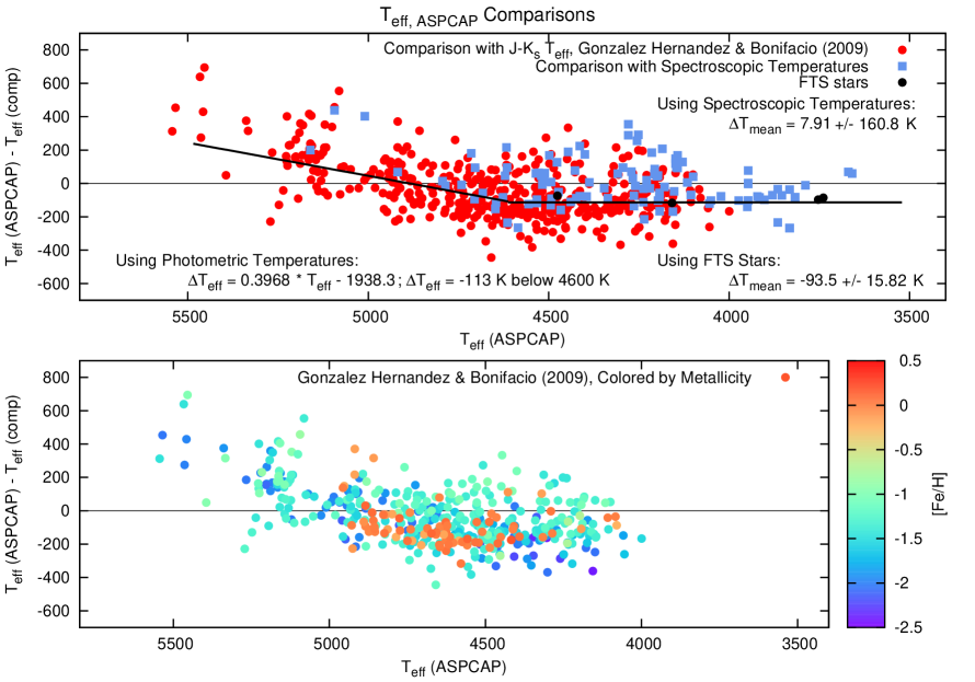
Figure 1: Top panel: ASPCAP effective temperatures compared to photometric calibrations (red squares), spectroscopic literature values (blue squares), and the four standard stars (black dots). The solid line represents the empirical calibration to the photometric temperatures. See Section 3.1 for discussion. Bottom panel: ASPCAP effective temperatures compared to photometric calibrations color coded by metallicity. Only giant stars with $\log~{}g$ $<$ 3.5 are plotted in both panels.

Figure 1 shows the differences between ASPCAP T_eff and $J-K_{s}$-based T_eff and those from other high-resolution spectroscopic studies. The agreement is generally good in both cases, however, there is a slight evidence of systematic offsets. The comparison with the photometric temperatures shows a linear trend in the differences as a function of ASPCAP T_eff between 4750 and 5500 K. Between 4600 and 5000 K, photometric (González Hernández & Bonifacio, 2009) and ASPCAP temperatures are in good agreement, although a slight trend towards higher ASPCAP T_eff is also visible. Below 4600 K, the ASPCAP temperatures are cooler than those based on $J-K_{s}$ by about 100$-$200 K. The photometric temperatures depend on the reddening used, thus for high reddening clusters ($E[B-V]>0.1$: M107, M71, NGC 2158, NGC 7789, NGC 6819, NGC 6791) errors in the reddening may lead to measurable linear shifts in the differences. An error of $\pm$10% in the reddening introduces an error of about $\pm$50 K in temperature, which is not enough to explain the differences between ASPCAP and the photometric scale by González Hernández & Bonifacio (2009), because our tests with zero reddening show that similar offsets remain. An additional error source is the zero point used in the calibration to the fundamental temperature scale, and we found that there is an average difference of 70 K between the calibrations of González Hernández & Bonifacio (2009) and the combined calibrations of Alonso et al. (1999, 2001); Houdashelt et al. (2000).

Despite these uncertainties we provide a calibration that ties ASPCAP temperatures to the scale used by González Hernández & Bonifacio (2009) between 4600 K and 5500 K:

$$T_{corrected} =T_{A}-0.3968\ T_{A}+1938.3 ;4600<T<5500$$

$$=T_{A}+113.3 ;3500<T<4600$$

where $T_{A}$ is the raw ASPCAP effective temperature. The equation is only valid for stars with $\log~{}g$ $<$ 3.5. Note that both the original spectroscopic $T_{\rm eff}$s and those calibrated with this relationship are provided in DR10.

The bottom panel of Figure 1 shows the metallicity dependence of the photometric scale comparison by color-coding the points according to metallicity. Below 5000 K both metal-poor and metal-rich stars are present, but no strong metallicity dependence can be perceived in the data. Above 5000 K the clusters presented in this paper only contain metal-poor stars, but expanding the comparison to field stars observed by APOGEE shows no metallicity dependence in this temperature range. However, because both metal-poor and metal-rich stars show large, 200$-$500 K differences above 5000 K, we believe that ASPCAP temperatures are overestimated in this region.

The comparison of the raw ASPCAP temperatures with the literature spectroscopic temperatures shows very good agreement for $T_{\rm eff}<5000$ K. The average difference is only 8 K, while the scatter is 161 K, of which a significant component could come from uncertainties in the literature values. The good agreement with spectroscopic gravities suggests that no empirical calibrations are required below 5000 K, which is in mild conflict with the photometric temperature comparison.

Comparing ASPCAP values with the fundamental (non-spectroscopic) temperatures from Smith et al. (2013) for the four standard stars, we find the latter to be warmer by an average of 94 $\pm 9$ K. This small discrepancy induces a metallicity difference between the two analyses of $-0.13\pm 0.03$ dex (see Section 3.2). These stars have well defined parameters, and the systematic difference of temperatures from ASPCAP agrees well with the photometric calibrations. We note that these stars were not observed by APOGEE, thus a simplified version of ASPCAP had to be used, which may introduce systematic differences, even if the spectral synthesis was based on the same line list and model atmosphere grid as for APOGEE.

In the end, we recommend using the corrected temperatures (equation 3) that bring the ASPCAP temperatures to the IRFM photometric scale. The advantage of doing so is that it is tied to the fundamental temperature scale, especially at solar abundance. Inspection of Figure 1 reveals a statistically significant but modest ($\sim$100 K) difference between the spectroscopic and fundamental scales. The precision of ASPCAP T_eff is discussed in more detail in Section 3.5.

3.2 Accuracy of Metallicity

Table 4: Properties of Clusters Derived from ASPCAP

ID	Name	N	[M/H]	[M/H]	[M/H] rms	Teff rms	[$\alpha$/H] rms
NGC 6341	M92	48	-2.03	-2.26	0.12	179.2	0.10
NGC 7078	M15	11	-2.11	-2.25	0.14	141.1	0.08
NGC 5024	M53	16	-1.94	-2.06	0.11	113.5	0.06
NGC 5466		8	-1.90	-2.02	0.08	135.1	0.06
NGC 4147		3	-1.66	-1.82	0.21	307.7	0.05
NGC 7089	M2	19	-1.46	-1.58	0.09	148.1	0.06
NGC 6205	M13	71	-1.43	-1.60	0.12	146.9	0.06
NGC 5272	M3	73	-1.39	-1.55	0.12	186.7	0.06
NGC 5904	M5	103	-1.19	-1.34	0.12	183.4	0.06
NGC 6171	M107	18	-0.92	-1.02	0.21	150.8	0.04
NGC 6838	M71	7	-0.72	-0.75	0.04	100.2	0.04
NGC 2158		10	-0.15	-0.17	0.03	101.7	0.02
NGC 2168	M35	1	-0.11	$\cdots$	$\cdots$	$\cdots$	$\cdots$
NGC 2420		9	-0.20	-0.22	0.04	64.0	0.03
NGC 188		5	+0.03	+0.06	0.02	123.1	0.02
NGC 2682	M67	24	+0.0	+0.03	0.06	64.8	0.03
NGC 7789		5	-0.02	+0.01	0.05	61.5	0.02
M45	Pleiades	75	-0.05	$\cdots$	0.18	$\cdots$	0.11
NGC 6819		30	+0.02	+0.05	0.06	77.8	0.02
NGC 6791		23	+0.25	+0.37	0.07	50.6	0.07

As any of the other primary physical parameters, metallicity is crucial for determining the rest of the abundances. In ASPCAP, the metallicity parameter ([M/H]) is used to track variations in all metal abundances locked in solar proportions, while deviations from solar abundance ratios are tracked by additional parameters, such as carbon, nitrogen and the alpha element abundances: [C/M], [N/M], and [$\alpha$/M], respectively (see Section 2.2). Here, we derive calibrations based on ASPCAP measurements of clusters with known metallicity. Since the adopted cluster metallicities are generally measurements of [Fe/H] (i.e., iron specifically), calibrations derived from these data tie ASPCAP [M/H] to literature values of [Fe/H]. For the most part, therefore, one can treat the calibrated values of [M/H] as if they were [Fe/H], and [X/M] values as [X/Fe]. Our tests in clusters also show that using only iron lines to derive [Fe/H] reproduces the uncalibrated [M/H] values to better than 0.1 dex. We maintain the M notation because the raw [M/H] values are derived fitting lines of many elements, not just iron. In following data releases we intend to publish individual abundances for many elements, including [Fe/H] (which would allow non-zero values of [Fe/M]), based on fittings to specific absorption lines in the APOGEE spectral window, establishing the detailed abundance pattern for each individual star.

The ASPCAP metallicities were compared to literature values cluster by cluster. Figure 2 (globular clusters) and 3 (open clusters) show the metallicity as a function of effective temperature for all the clusters examined in this paper. The average cluster metallicities adopted from the literature are listed in Table 1. Table 4 lists the average cluster ASPCAP metallicities and the standard deviation for each cluster.

Figure 2: [M/H] as a function of effective temperature derived with ASPCAP for globular clusters. Average cluster metallicities and the standard deviation of both the average and the distribution is labeled. Solid line marks the average of ASPCAP metallicities, the dashed line denotes the cluster average from literature, listed in Table 1. ASPCAP metallicities are 0.2$-$0.3 dex higher than the literature (Table 1.) below [M/H]=$-$0.7. A slight trend with temperature is visible in the data for some of the globular clusters. See Section 3.2 for discussion.

Figure 3: Same as Figure 2, but for open clusters. ASPCAP metallicities show good agreement (to within less than 0.1 dex) with the literature between [M/H]=$-$0.5 and [M/H]=$+$0.1, however at the very metal-rich end they are underestimated by about 0.2$-$0.3 dex. See Section 3.2 for discussion.

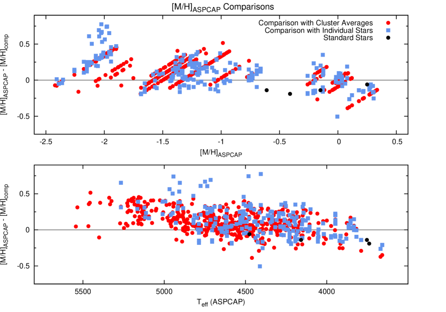
Figure 4: ASPCAP [M/H] is compared to individual star by star (blue squares) metallicities for cluster members, and standard stars (black). The differences from the cluster mean values are plotted with red dots as a function of ASPCAP [M/H] (upper panel) and T_eff (lower panel). Only giant stars with $\log~{}g$ $<$ 3.5 are plotted in both panels.

Figure 5: Left panels show the differences of raw ASPCAP metallicities and cluster averages plotted as a function of [M/H] (top) and T_eff (bottom). The solid line show the fitted relation (4) for 5500 K, and dotted lines show the same for 3500 K. Right panels show metallicities after calibration from 4 is applied. See Section 3.2 for discussion. Only giant stars with $\log~{}g$ $<$ 3.5 are plotted in all panels.

Near solar-metallicity, the raw metallicities derived from the APOGEE spectra are very close to the metallicities from the literature (Figure 3). Open clusters with $-0.5<$[M/H]$<0.1$ agree within 0.1 dex with the literature averages. In globular clusters below [M/H]$=-0.5$, the differences increase as [M/H] decreases, from systematic offsets of 0.1 dex for M71 to 0.35 for M92 (Figure 2). The reason that ASPCAP overestimates [M/H] at low metallicities may be related to the decreasing number of metal lines, and increasing number of $\alpha-$element lines (mostly OH), which leads to strong correlations between the two quantities (see Section 3.5). The metallicity also shows indication of linear trends as a function of T_eff for almost all globular clusters. This is mostly visible in M92, M2, and M13 (Figure 2). This dependence does not exist in the metal-rich open clusters. Stars above 5000 K show a significant systematic difference in T_eff (up to 200$-$500 K) compared to photometric temperatures, and this contributes to systematically different metallicities. This large temperature offset may combine with the error coming from the lack of Fe lines at low metallicities, and the two sources of errors together may lead to the overestimates of the metallicity and small linear trends with temperature.

Figure 4 shows the differences between raw ASPCAP metallicities and the literature values using both the literature cluster averages (red) as well as the measurements of individual cluster stars from the literature (blue). As expected, the trends are similar, given that the cluster averages are determined from the individual star measurements. Because the latter include star-by-star uncertainties, we chose to use the cluster averages as a basis to derive an empirical calibration to bring the raw ASPCAP metallicities onto the literature scale.

Figure 6: ASPCAP cluster average metallicities before (open circles) and after (filled circles) the correction. The corrected values lie within $\pm$ 0.1 dex from average literature values. The latter are listed in Table 1, while ASPCAP values are presented in Table 4.

The ASPCAP metallicities for the standard stars (black points in Figure 4) are too low compared with the analysis by Smith et al. (2013) by an average of 0.13 $\pm 0.03$ dex as a result of the average $-$93 K difference in temperature. According to Gray (1992, pp. 286-287), one might expect the abundances derived from neutral lines (like in the case of the standard stars) to have a dependence with temperature of $-1.3\times 10^{-3}$ dex K^-1 when the excitation potential is about 0 eV and $-0.4\times 10^{-3}$ dex K^-1 when it is about 5 eV. In our case a 93 K shift corresponds to 0.12 dex, and 0.04 dex respectively.

Within a given cluster, we found that the deviation of the ASPCAP metallicity from the literature value was also a function of effective temperature. The sensitivity to effective temperature is demostrated in the bottom panel of Figure 4. To account for both the metallicity and temperature dependence of the systematic errors in metallicity, we derived an empirical correction using both quantities as independent variables:

$$[M/H]_{corrected}=[M/H]_{A}+0.06199[M/H]_{A}^{2}-1.125\cdot 10^{-4}T_{A}+4.734\cdot 10^{-5}T_{A}[M/H]_{A}+0.544$$ (4)

where $[M/H]_{A}$ is the raw ASPCAP metallicity and $T_{A}$ is the raw ASPCAP effective temperature. The calibration is valid between $-$2.5 and 0.5 dex in metallicity, and from 3500 K to 5500 K in temperature for all stars with $\log~{}g$ $<$ 3.5.

Figure 5 shows the metallicities after this correction is applied, demonstrating that this relation does a good job of bringing the raw ASPCAP values into agreement with the literature values. Because of the temperature term, the overall scatter of the corrected differences is smaller as well, although some trends with temperature at low metallicities are still present. The scatter of the differences after the correction is 0.12 dex across the full metallicity range, which is only slightly larger than the scatter of the original values in each of the individual clusters (see Section 3.5). Figure 6 shows the cluster averages compared to the literature values before and after correction. Cluster averages in the full metallicity range are within $\pm$ 0.1 dex the literature after calibration.

3.3 Accuracy of Surface Gravity

Spectral features are generally less sensitive to surface gravity than to effective temperature or metallicity, so accurate values are challenging to derive. However, surface gravities are a critical ingredient for the estimation of spectroscopic parallaxes, therefore achieving the highest possible accuracy is important. Simulations based on photon noise-added synthetic spectra predict a floor of approximately 0.2 dex in $\log~{}g$ uncertainty for APOGEE spectra with S/N$\sim$100/pixel, although this is a function of effective temperature and metallicity.

3.3.1 Surface Gravity from Isochrones and Stellar Oscillations

To check the accuracy of our derived surface gravity, several types of independently derived gravities were used.

For cluster stars, theoretical isochrones can be used to provide a surface gravity for a given effective temperature, if the cluster age and distance are known. We derived gravities for our sample using isochrones from the Padova group (Bertelli et al., 2008, 2009), adopting cluster parameters as given in Table 1; because the Padova isochrones use scaled-solar abundances, we adopted isochrones with metallicities increased by 0.2 over the adopted [Fe/H] for the metal-poor globular clusters to account for the alpha-enhancement generally seen in these. We compared these results to those obtained using isochrones from the Dartmouth group (Dotter et al., 2008), and found that the derived surface gravities were within 0.1 dex, i.e. the differences are smaller than our expected random errors. For effective temperatures, we used the calibrated ASPCAP temperatures discussed above; as described below, the calibrated temperatures provided more consistent results than those obtained using the raw ASPCAP temperatures. We note, however, that surface gravities derived in using isochrones have significant uncertainties: they are correct only to the extent that model isochrones on the giant branch are accurate, and even then, since the giant branches are steep, a 100 K error in temperature leads to a 0.2$-$0.3 dex error in gravity depending slightly on metallicity.

The second method involves a comparison of ASPCAP gravities for stars in the Kepler field with those derived from asteroseismic analysis. These are expected to be highly accurate, with uncertainties of 0.01$-$0.03 dex. However, the Kepler stars do not include any metal-poor objects and thus do not span the full range of parameters of APOGEE stars.

Further verification of the surface gravities can be made by comparing the ASPCAP results with those determined by other spectroscopic studies for stars in which such data exist. However, log g values from the literature generally have significant uncertainties (up to 0.2$-$0.4 dex), so we believe that this approach provides poorer calibration than either isochrone or asteroseismic comparisons.

3.3.2 Empirical Calibration of Surface Gravity

In Figures 7 and 8, ASPCAP surface gravities and effective temperatures (red dots) are shown along with theoretical isochrones (blue line) for a number of globular and open clusters. Significant disagreement is apparent for the metal-poor globular clusters. We note that while the temperature correction discussed above would move the ASPCAP points into slightly better agreement with the isochrones, it is not large enough to account for the bulk of the discrepancy: ASPCAP surface gravities are inferred to be $\sim$ 0.5 dex too high for metal-poor stars. For the more metal-rich open clusters (Figure 8) the ASPCAP points fall closer to the isochrones, suggesting offsets of 0$-$0.3 dex in surface gravity.

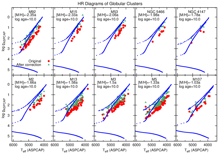
Figure 7: T${}_{\rm eff}-$ $\log~{}g$ diagrams of globular clusters. Metallicities denoted by ”a” in the labels were increased by 0.2 dex to account for the increased $\alpha$ content, and these increased values were used to generate the plotted isochrones. Red dots show the original ASPCAP $\log~{}g$ values as a function of ASPCAP T_eff. Isochrones and Kepler stars were used to calibrate ASPCAP gravities, and new values after the calibration described in Section 3.3 are plotted with green triangles.

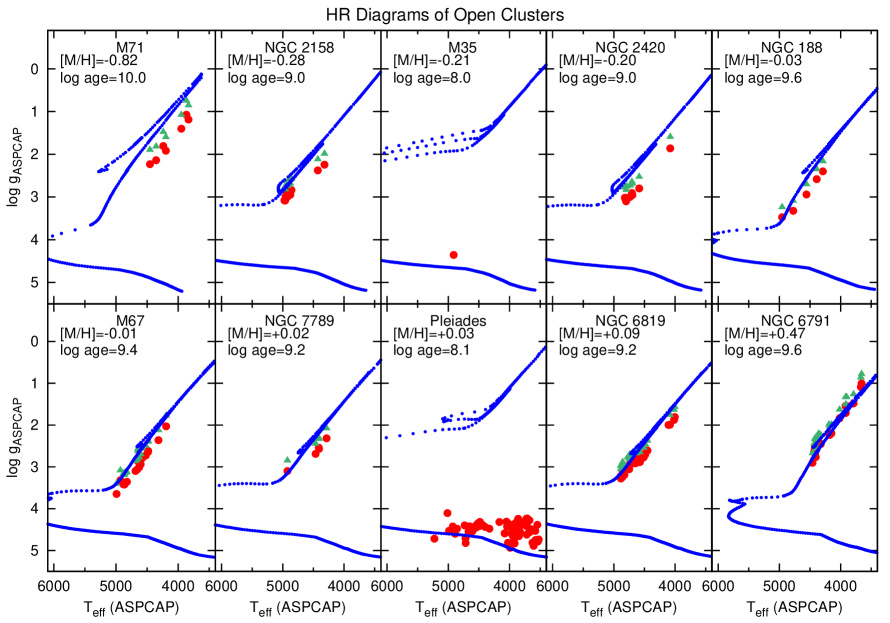
Figure 8: T${}_{\rm eff}-$ $\log~{}g$ diagrams of open clusters. For explanation please see the caption of Figure 7.

Comparison of ASPCAP and asteroseismic gravities for Kepler stars is shown in the upper panels of Figure 9, where the difference between the two sets of gravities is plotted against metallicity and effective temperature. This suggests that ASPCAP gravities are generally too high by a few tenths of a dex. Since, as noted above, the Kepler sample does not include more metal-poor stars, it cannot be used to confirm the larger discrepancies suggested by the isochrone comparison for metal-poor clusters. Figure 9 suggests that there is substantial scatter in the difference between ASPCAP and asteroseismic log g that is not well correlated with either metallicity or temperature, although there is certainly a trend with temperature for the bulk of the sample. Interestingly, the deviations appear to depend on evolutionary state of the star: red points denote stars that are asteroseismically determined to be hydrogen burning RGB stars, while blue points are helium burning red clump stars. We do not yet have a good explanation for this.

Generally, the inferred offsets in surface gravity are comparable using the isochrone gravities and the asteroseismic gravities, but there are some small inconsistencies. For the most metal-rich stars, the isochrones suggest that the ASPCAP surface gravities are nearly correct, while the asteroseismic analysis suggests that the ASPCAP gravities are still overestimated. In addition, the isochrone comparison does not suggest trends with effective temperature that appear for a large fraction of the Kepler sample. We note that small changes in the ASPCAP temperature scale or in adopted cluster parameters are unable to resolve these discrepancies. It is possible that they are related with the issues with evolutionary state.

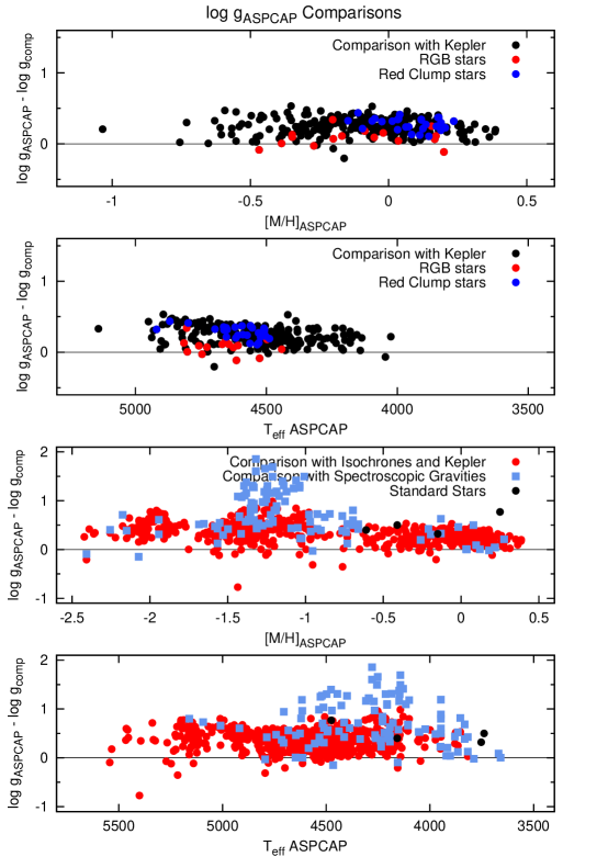
Figure 9: Top two panels: Comparison of ASPCAP log g with asteroseismic log g for stars in the Kepler fields. Top panel shows differences as a function of ASPCAP metallicity, while bottom panel shows differences as function of temperature. Red points are asteroseismically confirmed giants, while blue points are asteroseismically confirmed red clump stars, while the evolutionary status of stars denoted by black dots are not yet confirmed. Bottom two panels: ASPCAP gravity differences compared to isochrones and Kepler stars (red dots), spectroscopic $\log~{}g$ (blue squares), and standard stars (black dots) are plotted as a function of [M/H] (upper panel) and T_eff (lower panel). In case of the isochrones, corrected temperature were used to determine the comparison value of surface gravity. Only giant stars with $\log~{}g$ $<$ 3.5 are plotted in all panels.

Figure 10: Comparison of ASPCAP log g with the combined dataset of asteroseismic and isochrone surface gravities. The applied empirical correction is shown on the left panels. Results after the empirical calibration are shown on the right panels. Values after the correction results in a 0.17 dex scatter covering the full metallicity and temperature range. See Section 3.3 for discussion. Only giant stars with $\log~{}g$ $<$ 3.5 are plotted in both panels.

To derive a calibration relation for surface gravity, we adopt a combined sample of Kepler stars with asteroseismic surface gravities and metal-poor cluster stars with isochrone surface gravities; specifically, we use all of the Kepler stars with $[M/H]>-1$ and all of the clusters with $[M/H]<-0.5$ (so there is an overlap region where both clusters and Kepler stars are used). We used corrected temperatures to determine gravities from isochrones, because adoption of original ASPCAP values increases the disagreement with seismic gravities.

The lower two panels of Figure 9 show how the $\log~{}g$ differences depend on metallicity and T_eff for this sample, and also includes a comparison of ASPCAP gravities with independently derived optical spectroscopic gravities from the literature (blue points) and from the fundamental (based on parallaxes) values for the standard stars (black dots in the two bottom panels of Figure 9., Smith et al., 2013). These generally agree with the differences inferred from isochrone and asteroseismic analysis, although there is significant scatter. The standard stars show no significant trends with metallicity or temperature, and an average difference of $0.48\pm 0.08$ dex, but we have to note that the gravity of $\mu$ Leo derived by Smith et al. (2013) is 0.77 dex lower than that determined by ASPCAP; this is a much larger deviation than suggested by any other data at this metallicity.

We adopt a gravity correction that is a function of metallicity only, as including any other independent variables is unable to improve the agreement. Fitting the observed differences yielded the empirical calibration relation:

$$\log~{}g_{corrected}=\log~{}g_{A}+0.1222[M/H]_{A}-0.2396$$ (5)

where [M/H]_A is the raw ASPCAP metallicity and $\log~{}g_{A}$ is the raw ASPCAP surface gravity.

Figure 10 presents the values before (left panels) and after (right panels) the calibration. For all metallicities and for T_eff between 3800 and 5500 K, this empirical correction reduces most of the systematic differences to around zero. The RMS scatter of the gravity differences compared with isochrones and Kepler gravities is reduced to 0.17 dex. We attempted to derive a calibration relation using other functional forms, but we found that the above solution gave the smallest standard deviation. We recommend that this relation be used, but with application limited to $3800<T_{A}<5500$ K, $-2.5<$[M/H]$<0.5$ dex, and $\log~{}g<3.5$.

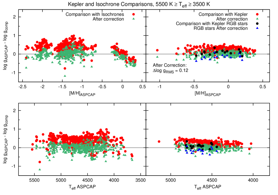
Figure 11: The calibration from Figure 10 applied to only isochrone differences (left panels), and to the Kepler sample (right panels). Some discrepancy remain at solar metallicities, where the calibration results in poor agreement with isochrone surface gravities in open clusters. Confirmed Kepler RGB stars (Mosser et al., 2011) are also plotted before (black dots) and after calibration (blue triangles). The evolutionary state classifications were done by Stello et al. (2013). Only giant stars with $\log~{}g$ $<$ 3.5 are plotted in all panels.

As a sanity check, in Figure 11 we compare the application of this calibration separately to the isochrone gravities (left panels) and to asteroseismic gravities (right) panels. The RMS scatter is only 0.12 dex after the correction for the Kepler stars, which is a significant improvement. The error in surface gravity shows a small dependence on temperature (Figure 11 lower right panel); this trend remains after application of the calibration relation. The discrepancy between corrections based on isochrone and asteroseismic gravity at high metallicity is evident in the left panel, where the corrected values show some disagreement with the isochrone gravities, in particular at the highest metallicities.

Figures 7 and 8 show the corrected points in the HR diagrams as green triangles. The corrected values are closer to the isochrones, but some discrepancies still remain, especially at low metallicities around [M/H]=$-$1 to $-$1.5 in M5, M3, and M13 (Figure 7, lower panels), and at high metallicities above +0.2 dex in NGC 6791 (Figure 8 lower right panel).

3.4 Accuracy of $\alpha-$elements, Carbon and Nitrogen Abundances

Figure 12: ASPCAP [$\alpha$/M] as a function of metallicity for globular clusters. Strong correlations between the two parameters is visible in all globular clusters.

Besides effective temperature, metallicity and gravity, three other parameters are also published in DR10: $\alpha-$elements, carbon, and nitrogen abundances. These six parameters are are simultaneous derived by ASPCAP. Figures 12 and 13 show [$\alpha$/M] as a function of metallicity for the globular and open clusters. In the metallicity region important for APOGEE ([M/H] $>-$0.5 and $<+$0.1), the derived $\alpha$ abundances show no trend in individual stars within a cluster with either metallicity, or temperature. However, strong dependencies are present as a function of [M/H], as well as T_eff (not shown), both below [M/H] = $-$0.5 (shown in M13, M5 for example) and above [M/H] = $+$0.1 (shown in NGC 6791). The trend in NGC 6791 is not supported by other observations, as abundances of $\alpha-$elements in NGC 6791 from the literature (Origlia et al., 2006; Carraro et al., 2006) are between [$\alpha$/M]=$-$0.1 and +0.1 dex, which indicates no $\alpha$ enrichment in this cluster.

Figure 13: ASPCAP [$\alpha$/M] as a function of metallicity for open clusters. The [$\alpha$/M] abundances close to solar metallicities show low scatter and have no visible dependence on metallicity or temperature.

Figure 14: C and N abundances compared to literature values. Metal poor clusters below [M/H] $<-1$ are marked with solid circles, while metal-rich clusters above -1 are denoted by open circles. See Section 3.4 for discussion.

Some of the above ambiguities may be due to the paucity and the weakness of metal lines in the spectra of metal-poor stars. Since few iron lines are visible while OH lines remain strong in metal-poor stars, the strength of the OH lines can be similarly matched by increasing [M/H] or $[\alpha$/H]. This situation is illustrated in Figure 12, where an anti-correlation between [$\alpha/$Fe] and [M/H] is apparent for example in the clusters M13 and M5. This effect is likely caused by correlated errors in metallicity and $\alpha$ abundances for NGC 6791.

The carbon and nitrogen abundance comparisons with literature values are shown in Figure 14; Table 1 lists the references used for the literature values. Carbon abundances are significantly overestimated for globular clusters (up to 1 dex), while for open clusters the agreement is better between [C/M] = $-$0.5 and 0. Nitrogen abundances are generally underestimated compared to other studies by about 0.2$-$0.4 dex at low nitrogen content, and up to 1 dex for stars with high nitrogen content. The overestimate of [N/M] at high [C/M] values may be a consequence of deriving nitrogen from CN: if ASPCAP underestimates [C/M] (as shown in the upper panel for [C/M] $>$ 0), [N/M] will thus be overestimated. We note that these comparisons are affected by the relative paucity of [C/Fe] and [N/Fe] data for cluster stars in the literature and by their intrinsic uncertainties, particularly in the case of nitrogen. Therefore, it is difficult to decide how much of the large scatter and zero point differences seen in Figure 14 is contributed by the APOGEE data, and how much by the literature data. Because of this uncertainty, we suggest that the current carbon and nitrogen abundances derived by ASPCAP be used with extreme caution. While the uncertainties in the C and N abundances may contribute to systematic effects in other derived parameters, in ways that are still not entirely understood, these possible systematics have been approximately removed by the calibration process presented in this paper. Thus, we expect the calibrated values for effective temperature, surface gravities, metallicities, and $\alpha$-element abundances to be free of any important systematic effects.

We believe that by defining certain spectral windows in the H-band for all these elements, along with other ASPCAP improvements, is likely to significantly improve the quality of the abundance determinations for these elements.

3.5 Precision of Effective Temperature, Metallicity, and $\alpha-$elements

ASPCAP provides formal internal error estimates for stellar parameters that are presently unrealistically small. The scatter within individual clusters offers an external estimate of uncertainties, which we adopt for T_eff and metallicity. The precision of the effective temperatures was calculated using the differences compared to the $J-K_{s}$ calibrations. Any systematic shifts were neglected by fitting a constant value to the differences. The error in temperature for each cluster was then calculated by determining the RMS scatter around this fit. The calculated uncertainties are shown in the right panel of Figure 15, and listed in Table 4. The overall scatter in temperature is less than 200 K, but it appears to be significantly better for metal-rich stars, where it is generally smaller than 100 K. A linear fit was used to characterize how the precision depends on metallicity, and the following function was adopted to estimate the ASPCAP temperature errors:

$$T_{eff,RMS}=-39.8\ [M/H]_{A}+83.8$$ (6)

where [M/H]_A is the raw ASPCAP metallicity. The equation is valid for stars with $\log~{}g$ $<$ 3.5.

Figure 15: The RMS of [M/H], [$\alpha$/M] and T_eff for each cluster (based on stars with $\log~{}g$ $<$ 3.5) as a function of uncorrected cluster average metallicity from ASPCAP. A linear empirical calibration was used in case of effective temperature and metallicity. See Section 3.5 for discussion.

The RMS scatter of metallicity, shown by circles in the left panel of Figure 15, was again determined by calculating the standard deviation around the cluster average values. The scatter in metallicity, in the range 0.08$-$0.14 dex for globular clusters, is higher for the most metal-poor clusters. For all the open clusters, with a nearly solar metallicity, the scatter is smaller, at about 0.03$-$0.07 dex. The average scatter using all clusters is 0.09 dex. There is one outlier cluster, M107, in which the scatter is 0.21 dex. This might be the result of possible uncertainties in metallicity above 5000 K, due to increased temperature offsets from photometric values. All other derived atmospheric parameters for M107 behave just like the other globular clusters. The RMS for the ensemble of clusters clearly depends on the metallicity, thus again a linear equation was used to estimate the ASPCAP metallicity errors:

$$[M/H]_{RMS}=-0.0361\ [M/H]_{A}+0.0548$$ (7)

The equation is valid for stars with $\log~{}g$ $<$ 3.5. The RMS of the $\alpha$ abundances, shown as squares in the left panel of Figure 15, are relatively low, of the order of 0.1 dex. Similarly to the metallicity, the $\alpha$ precision gets worse with decreasing metallicity due to the metallicity-$\alpha$ correlation found in the globular clusters. Near solar metallicities, the typical error spans between 0.02 and 0.07 dex, with no systematic deviations as a function of metallicity or temperature. Because the RMS increases due to systematics in the metallicity-$\alpha$ correlation, we do not fit the RMS the of $\alpha$ abundances. We believe that the true random error of $\alpha$ is smaller than what is presented for the metal-poor stars.

3.6 Future Improvements

We plan several improvements in how we will obtain the physical parameters for APOGEE’s next data release (DR12, planned for December 2014). This section provides an overview on those ongoing developments.

The model atmospheres used in the current (DR10) version of ASPCAP are those published by Castelli $\&$ Kurucz (2003) based on the ATLAS9 code (Kurucz, 1979). We have recently produced an updated grid of model atmospheres based on the most recent version of ATLAS9 (Meszaros et al., 2012), including an updated H₂ line list. The new grid of models considers, in addition to the usual variations in metal abundance, variations in $\alpha$-element enhancement and carbon abundance [C/M], which will lead to a spectral library with consistent abundances between the synthesis and the model atmospheres.

The [$\alpha$/M]$-$[M/H] correlation found in metal-poor and metal-rich clusters can be improved by separating iron lines from OH lines and fitting them separately. This will lead to a more simple fit, where in the first step the metallicity is determined from iron lines, and in a second step $\alpha$ abundances can be derived from OH, and other $\alpha$-element lines.

We have clearly shown that our spectroscopic surface gravities differ systematically from those derived from isochrones or stellar oscillations. One or several of the many approximations involved in the calculation of model spectra are likely behind these systematic errors. Departures from LTE, enhanced by the low densities found in the atmospheres of giant stars, could be affecting some of the atomic populations. Molecular populations are quite sensitive to the thermal structure in high atmospheric layers, and also to thermal inhomogeneities that must be present in the real stars, and these are completely neglected in our 1D model atmospheres, and the main suspect for the observed systematic offsets.

We have already started to look at how to bring ASPCAP gravities into better agreement with asteroseismic gravities. Grids of hydrodynamical model atmospheres are becoming available, and we plan to examine their impact on the H-band spectrum of giants in the near future (Chiavassa et al., 2011; Collet et al., 2007; Freytag et al., 2012; Ludwig et al., 2009). We have also noticed that the Brackett series lines in the spectra, which are fairly sensitive to pressure, are not always well matched by our model spectra, and their modeling may need to be revised.

While the overall size of the differences between our spectroscopic gravities and those from isochrones or pulsations are similar, we have identified some discrepancies when comparing ASPCAP surface gravities with these two independent sources. We will examine closely these inconsistencies to identify the reasons behind them. Among the candidates we plan on exploring are the effects of the mixing length and other convection parameters as well as the helium content in the construction of stellar evolution models. We will also closely evaluate the applicability of the adopted scaling relationship between the frequency of maximum power of oscillations ($\nu_{\rm max}$) and the surface gravity.

The ASPCAP analysis has so far been restricted to the main atmospheric parameters and the abundances of C, N and overall abundances of $\alpha$-elements and metals. We are further developing ASPCAP to handle the derivation of abundances for many more elements accessible from the H-band. Our preliminary studies indicated that up to 15 different elements are well represented in this spectral window for late-type giant stars (Eisenstein et al., 2011).

As part of these improvements, a manual analysis is being carried out for a number of the ASPCAP calibration clusters. These analyses will include derivations of the fundamental atmospheric parameters themselves, as well as measuring the additional 15 elements that are part of the APOGEE survey plan. These results will be used to further refine and calibrate the ASPCAP pipeline.

4 Summary

We have used data of 559 stars belonging to 20 Galactic globular and open clusters or with high-quality asteroseismic data to determine the accuracy and precision of atmospheric parameters published in DR10. The APOGEE spectra were run through the current version of the APOGEE Stellar Parameters and Stellar Abundances Pipeline (ASPCAP), and cluster members were selected carefully to compare effective temperature, metallicity, surface gravity, $\alpha$-elements, carbon and nitrogen abundances to literature values.

After carefully examining all six derived parameters we concluded the following:

Effective temperature: Effective temperatures agree well with spectroscopic temperatures from the literature within a mean offset of 8$\pm$161 K. For photometric temperatures, larger systematic differences can be seen. A correction function was provided to convert ASPCAP temperatures to the photometric scale of González Hernández & Bonifacio (2009), which is based on the IRFM method. The precision of ASPCAP temperatures was estimated using the RMS scatter of the clusters, and it is found to be about 150$-$200 K in globular clusters, and 50$-$100 K in open clusters at solar metallicities.

Metallicity: ASPCAP metallicities agree very well (to within 0.1 dex) with literature values for stars with $-0.5<$ [M/H] $<+0.1$ dex. At both the metal-poor and metal-rich ends of the scale, systematic differences are apparent, amounting up to 0.2$-$0.3 dex. An empirical correction is provided using literature cluster averages to bring ASPCAP metallicities into agreement with the literature values. The metallicity scatter in each individual cluster is usually less than 0.15 dex, while the average scatter in all 20 clusters is 0.09 dex.

Gravity: ASPCAP gravities are larger by about 0.2$-$0.3 dex than both isochrones and seismic values for metallicity in the range $-0.5<$ [M/H] $<+0.1$ dex. At lower metallicities the difference is larger. An empirical correction is provided based on a combined data set including isochrone comparisons for metal-poor stars and Kepler seismic values at solar metallicities.

$\alpha$ abundances: [$\alpha$/M] abundances for stars within $-0.5<$ [M/H] $<+0.1$ dex show no dependence on temperature, or metallicity. However, a clear correlation exists with [M/H] and T_eff outside this metallicity range, thus we advice to use $\alpha$ abundances with caution for stars with $-0.5>$ [M/H] and $>+0.1$ dex. The typical precision in the above mentioned region is less than 0.07 dex. In addition, we are not confident on the derived [$\alpha$/M] results for $T_{\rm eff}lessim4200$ K.

Carbon and nitrogen: The carbon and nitrogen abundances show significant systematic differences (up to 1 dex) compared to literature values. We currently discourage any use of those values in scientific applications.

Further developments of ASPCAP will be available in the near future and aim to reduce the systematic effects seen in metallicity and gravity. The new data set with improved atmospheric parameters will be available in DR12, at the end of 2014. Continued improvements in the processing and analysis of APOGEE spectra will no doubt be one of the highest priorities for the APOGEE team in the upcoming years.

References

- Aihara et al. (2011) Aihara, H., Allende Prieto, C., An, D. et al. 2011, ApJS, 193, 29
- Ahn et al. (2013) Ahn, C. P., Alexandroff, R., Allende Prieto, C. et al. 2013, submitted to AJ
- Allende Prieto (2008) Allende Prieto, C. 2008, Physica Scripta Volume T, 133, 014014
- Allende Prieto et al. (2006) Allende Prieto, C., Beers, T. C., Wilhelm, R., et al. 2006 ApJ, 636, 804
- Allende Prieto et al. (2003) Allende Prieto, C., Lambert, D. L., Hubeny, I., Lanz, T. 2003, ApJS, 147, 363
- Alonso et al. (1999) Alonso, A., Arribas, S., & Martínez-Roger, C. 1999, A&AS, 140, 261
- Alonso et al. (2001) Alonso, A., Arribas, S., & Martínez-Roger, C. 2001, A&A, 376, 1039
- Basu et al. (2010) Basu, S., Chaplin, W. J., & Elsworth, Y. 2010, ApJ, 710, 1596
- Barrado et al. (2001) Barrado y Navascués, D., Deliyannis, C. P., & Stauffer, J. R. 2001, ApJ, 549, 452
- Bertelli et al. (2008) Bertelli, G., Girardi, L., Marigo, P., & Nasi, E. 2008, A&A, 484, 815
- Bertelli et al. (2009) Bertelli, G., Nasi, E., Girardi, L., & Marigo, P. 2009, A&A, 508, 355
- Borucki et al. (2010) Borucki, W.J., Koch, D., Basri, G. et al. 2010, Science, 327, 977
- Bragaglia et al. (2001) Bragaglia, A., Carretta, E., Gratton, R. G. et al. 2001, AJ, 121, 327
- Briley et al. (1997) Briley, M. M., Smith, V. V., King, J., & Lambert, D. L. 1997, AJ, 113, 306
- Carraro et al. (2006) Carraro, G., Villanova, S., Demarque, P. et al. 2006, ApJ, 643, 1151
- Carretta et al. (2007) Carretta, E., Bragaglia, A.,& Gratton, R. G. 2007, A&A, 473, 129
- Carretta et al. (2009) Carretta, E., Bragaglia, A., Gratton, R., D’Orazi, V., & Lucatello, S. 2009, A&A, 508, 695
- Casagrande et al. (2010) Casagrande, L., Ramírez, I., Meléndez, J., Bessell, M., & Asplund, M. 2010, A&A, 512, 54
- Cassisi et al. (2006) Cassisi, S., Pietrinferni, A., Salaris, M. et al. 2006, Mem. Soc. Astron. Italiana, 77, 71
- Castelli Kurucz (2003) Castelli, F., Kurucz, R. L. 2003, New Grids of ATLAS9 Model Atmospheres, IAUS, 210, 20P
- Cavallo & Nagar (2000) Cavallo, R. M., & Nagar, N. M. 2000, AJ, 120, 1364
- Chiavassa et al. (2011) Chiavassa, A., Pasquato, E., Jorissen, A. et al. 2011, A&A, 528, A120
- Collet et al. (2007) Collet, R., Asplund, M., & Trampedach, R. 2007, A&A, 469, 687
- Creevey & Thévenin (2012) Creevey, O. L. & Thévenin, F. 2012, in SF2A-2012: Proceedings of the Annual meeting of the French Society of Astronomy and Astrophysics, ed. S. Boissier, P. de Laverny, N. Nardetto, R. Samadi, D. Valls-Gabaud, & H. Wozniak, 189–193
- Creevey et al. (2013) Creevey, O. L., Thévenin, F., Basu, S. et al. 2013, MNRAS, 431, 2419
- Cohen & Meléndez (2005) Cohen, J. G., & Meléndez, J. 2005, AJ, 129, 303
- Cunha & Smith (2006) Cunha, K. & Smith, V.V. 2006, ApJ, 651, 491
- Cutri et al. (2003) Cutri. R.M., et al. 2003, The IRSA 2MASS All-Sky Point Source Catalog, NASA/IPAC Infrared Science Archive
- Dalton et al. (2012) Dalton, G., Trager, S. C., Abrams, D. C. et al. 2012, Proc. SPIE, 8446
- Demarque et al. (2004) Demarque, P., Woo, J.-H., Kim, Y.-C., & Yi, S. K. 2004, ApJS, 155, 667
- Dotter et al. (2008) Dotter, A., Chaboyer, B., Jevremović, D. et al. 2008, ApJS, 178, 89
- Dotter et al. (2007) Dotter, A., Chaboyer, B., Jevremović, D. et al. 2007, AJ, 134, 376
- Eisenstein et al. (2011) Eisenstein, D. J., Weinberg, D. H., Agol, E. et al. 2011, AJ, 142, 72
- Freeman (2012) Freeman, K. C. 2012, Galactic Archaeology: Near-Field Cosmology and the Formation of the Milky Way, 458, 393
- Freytag et al. (2012) Freytag, B., Steffen, M., Ludwig, H.-G. et al. 2012, Journal of Computational Physics, 231, 919
- Friel et al. (2002) Friel, E. D., Janes, K. A., Tavarez, M. et al. 2002, AJ, 124, 2693
- Gai et al. (2011) Gai, N., Basu, S., Chaplin, W. J., & Elsworth, Y. 2011, ApJ, 730, 63
- García et al. (2011) García, R. A., Hekker, S., Stello, D. et al. 2011, MNRAS, 414, L6
- Gilmore et al. (2012) Gilmore, G., Randich, S., Asplund, M. et al. 2012, The Messenger, 147, 25
- González Hernández & Bonifacio (2009) González Hernández, J. I., & Bonifacio, P. 2009, A&A, 497, 497
- Gratton et al. (2004) Gratton, R., Sneden, C. & Carretta, E. 2004, ARA&A, 42, 385
- Gray (1992, pp. 286-287) Gray, D. F. 1992, The Observation and Analysis of Stellar Photospheres, (Cambridge: Cambridge Univ. Press)
- Gunn et al. (2006) Gunn, J. E., Siegmund, W. A., Mannery, E. J. et al. 2006, AJ, 131, 2332
- Ivans et al. (2001) Ivans, I. I., Kraft, R. P., Sneden, C. S., et al. 2001, AJ, 122, 1438
- Jacobson et al. (2011) Jacobson, H. R., Pilachowski, C. A., & Friel, E. D. 2011, AJ, 142, 59
- de Jong et al. (2012) de Jong, R.S. Bellido-Tirado, O., Chiappini, C. et al. 2012, SPIE, 8466
- Harris 1996 (2010 edition) Harris, W.E. 1996, AJ, 112, 1487
- Hekker et al. (2010) Hekker, S., Broomhall, A.-M., Chaplin, W. J., et al. 2010, MNRAS, 402, 2049
- Hekker et al. (2012) Hekker, S., Elsworth, Y., & Mosser, B. 2012, A&A, 544, 90
- Houdashelt et al. (2000) Houdashelt, M. L., Bell, R. A., & Sweigart, A. V. 2000, AJ, 119, 1448
- Kalirai et al. (2001) Kalirai, J. S., Richer, H. B., Fahlman, G. G. et al. 2001, AJ, 122, 266
- Kallinger et al. (2010) Kallinger, T., Mosser, B., Hekker, S. et al. 2010, A&A, 522, 1
- Koch & McWilliam (2010) Koch, A., & McWilliam, A. AJ, 139, 2289
- Koesterke (2009) Koesterke, L. 2009, American Institute of Physics Conference Series, 1171, 73
- Koesterke et al. (2008) Koesterke, L., Allende Prieto, C. Lambert, D. L. 2008, ApJ, 680, 764
- Kraft & Ivans (2003) Kraft, R. P., & Ivans, I. I. 2003, PASP, 115, 143
- Kraft et al. (1992) Kraft, R. P., Sneden, C., Langer, G. E., & Prosser, C. F. 1992, AJ, 104, 645
- Kunder et al. (2012) Kunder, A., Koch, A., Rich, R. M. et al. 2012, AJ, 143, 57
- Kurucz (1979) Kurucz, R. L. 1979, ApJS, 40, 1
- Lai et al. (2010) Lai, D. K., Bolte, M., Johnson, J. A. et al. 2010, ApJ, 722, 1984
- Lee et al. (2004) Lee, J.-W., Carney, B. W., & Balachandran, S. C. 2004, 128, 2388
- Lindegren (2010) Lindegren, L. 2010, IAU Symp., 261, 296
- Ludwig et al. (2009) Ludwig, H.-G., Caffau, E., Steffen, M. et al. 2009, Mem. Soc. Astron. Italiana, 80, 711
- Majewski et al. (2013) Majewski, S.R. et al. 2013, in prep.
- Marigo et al. (2008) Marigo, P., Girardi, L., Bressan, A. et al. 2008, A&A, 482, 883
- Meléndez et al. (2001) Meléndez, J., Barbuy, B. & Spite, F. 2001, ApJ, 556, 858
- Meléndez & Cohen (2009) Meléndez, J. & Cohen, J. G. 2009, ApJ, 699, 2017
- Meszaros et al. (2012) Meszaros, Sz., Allende Prieto, C., Edvardsson, B. et al. 2012, AJ, 144, 120
- Minniti et al. (1996) Minniti, D., Peterson, R. C., Geisler, D., & Claria, J. J. 1996, 470, 953
- Morel & Miglio (2012) Morel, T. & Miglio, A. 2012, MNRAS, 419, L34
- Mosser & Appourchaux (2009) Mosser, B., & Appourchaux, T. 2009, A&A, 508, 877
- Mosser et al. (2011) Mosser, B., Barban, C., Montalbán, J. et al. 2011, A&A, 532, A86
- Ness et al. (2012a) Ness, M., Freeman, K. & Athanassoula, E. 2012a, ASPC, 458, 195
- Ness et al. (2012b) Ness, M., Freeman, K., Athanassoula, E. et al. 2012b, ApJ, 756, 22
- Nidever et al. (2013) Nidever, D.L. et al. 2013, in preparation
- O’Connell et al. (2011) O’Connell, J. E., Johnson, C. I., Pilachowski, C. A., & Burks, G. 2011, PASP, 123, 1139
- Origlia et al. (2002) Origlia, L. Rich, R.M. & Castro, S. 2002, AJ, 123, 1559
- Origlia et al. (2006) Origlia, L., Valenti, E., Rich, R. M., & Ferraro, F. R. 2006, ApJ, 646, 4990
- Otsuki et al. (2006) Otsuki, K., Honda, S., Aoki, W., Kajino, T. & Mathews, G. J. 2006, ApJ, 641, L117
- Pancino et al. (2010) Pancino, E., Carrera, R., Rossetti, E., & Gallart, C. 2010, A&A, 511, 56
- Perryman et al. (2001) Perryman, M.A.C., de Boer, K.S., Gilmore, G. et al. 2001, A&A, 369, 339
- Pinsonneault et al. (2012) Pinsonneault, M. H., An, D., Molenda-Żakowicz, J. et al. 2012, ApJS, 199, 30
- Press et al. (1992) Press, W. H., Teukolsky, S. A., Vetterling, W. T., Flannery, B. P. 1992, Numerical Recipes in Fortran 77: the art of scientific computing, 2nd edition, Cambridge Univ. Press
- Ramírez & Cohen (2003) Ramírez, S. V. & Cohen, J. G. 2003, AJ, 125, 224
- Roederer & Sneden (2011) Roederer, I. U. & Sneden, C. 2011, AJ, 142, 22
- Ryde et al. (2010) Ryde, N., Gustafsson, B., Edvardsson, B. et al. 2010, A&A, 509, A20
- Shetrone (1996) Shetrone, M. D. 1996, AJ, 112, 1517
- Shetrone et al. (2010) Shetrone, M., Martell, S. L., Wilkerson, R. et al. 2010, AJ, 140, 1119
- Schlegel et al. (1998) Schlegel, D. J., Finkbeiner, D. P., & Davis, M. 1998, ApJ, 500, 525
- Smith et al. (2013) Smith, V. V., Cunha, K., Shetrone, M. D. et al. 2013, ApJ, 765, 16
- Sneden (1973) Sneden, C. 1973, PhD thesis, Univ. Texas at Austin
- Sneden et al. (2000) Sneden, C., Pilachowski, C. A., & Kraft, R. P. 2000, AJ, 120, 1351
- Sneden et al. (2004) Sneden, C., Kraft, R. P., Guhathakurta, P., Peterson, R. C., & Fulbright, J. P. 2004, 127, 2162
- Sneden et al. (1991) Sneden, C., Kraft, R. P., Prosser, C. F., & Langer, G. E. 1991, AJ, 102, 2001
- Sneden et al. (1992) Sneden, C., Kraft, R. P., Prosser, C. F., & Langer, G. E. 1992, AJ, 104, 2121
- Sneden et al. (1997) Sneden, C., Kraft, R. P., Shetrone, M. D. et al. 1997, AJ, 114, 1964
- Sobeck et al. (2011) Sobeck, J. S., Kraft, R. P., Sneden, C. et al. 2011, AJ, 141, 175
- Soderblom et al. (2009) Soderblom, D. R., Laskar, T., Valenti, J. A., Stauffer, J. R., & Rebull, L. M. 2009, AJ, 138, 1292
- Steinmetz et al. (2006) Steinmetz, M., Zwitter, T., Siebert, A. et al. 2012, AJ, 132, 1645
- Stello et al. (2013) Stello et al. 2013, arXiv, 1302.0858
- Strutskie et al. (2006) Strutskie, M.F. et al. 2006, AJ, 131, 1163
- Tautvaišiene et al. (2005) Tautvaišiene, G., Edvardsson, B., Puzeras, E., & Ilyin, I.
- Tautvaišiene et al. (2000) Tautvaišiene, G., Edvardsson, B., Tuominen, I. & Ilyin, I. 2000, A&A, 360, 499
- Thygesen et al. (2012) Thygesen, A. O., Frandsen, S., Bruntt, H., et al. 2012, A&A, 543, A160
- Wilson et al. (2012) Wilson, J., Hearty, F., Skrutskie, M. F. et al. 2012, SPIE, 8446, 84460H
- Yanny et al. (2009) Yanny, B. Newberg, H. J., Johnson, J. A. et al. 2009, ApJ, 700, 1282
- Yong et al. (2006) Yong, D., Aoki, W., & Lambert, D. L. 2006, 638, 1018
- Yong et al. (2008) Yong, D., Karakas, A. I., Lambert, D. L., Chieffi, A., Limongi, M. 2008, 689, 1031
- Zasowski et al. (2013) Zasowski, G., Johnson, J. A., Frinchaboy, P. M. et al. 2013, arXiv, 1308.0351
- Zhao et al. (2006) Zhao, G., Chen, Y.-Q., Shi, J.-R., et al. 2006 ChJAA, 6, 265