A conservative, skew-symmetric Finite Difference Scheme for the compressible Navier–Stokes Equations

Abstract

We present a fully conservative, skew-symmetric finite difference scheme on transformed grids. The skew-symmetry preserves the kinetic energy by first principles, simultaneously avoiding a central instability mechanism and numerical damping. In contrast to other skew-symmetric schemes no special averaging procedures are needed. Instead, the scheme builds purely on point-wise operations and derivatives. Any explicit and central derivative can be used, permitting high order and great freedom to optimize the scheme otherwise. This also allows the simple adaption of existing finite difference schemes to improve their stability and damping properties.

Keywords: Compressible Flows; Skew-Symmetry; Conservative Finite Differences; Summation by Parts

1 Introduction

Flows featuring shocks and acoustics are common in engineering applications. Examples are the sound generation of supersonic jets, noise generation in transonic flight or shock buffeting on an airfoil, where one possible mechanism is the interaction of sound waves from the trailing edge with the standing shock on the airfoil.

Simulations of such configurations are numerically challenging as the correct and stable simulation of shocks and the faithful calculation of acoustics have different, and in standard approaches, contradictory requirements. Shocks, on the one hand, are described by the Rankine-Hugoniot conditions, which build directly on the conservation laws. Conservation of mass, momentum and total energy is a prerequisite to guarantee a correct shock treatment. Such conserving schemes are usually finite volume (FV) schemes.

Acoustics, on the other hand, are propagating disturbances. They experience very low damping and travel long distances without noticeable energy loss in practice. When the amplitude is small the dispersion is also very small. To preserve these properties in a numerical simulation, schemes with very low (numerical) damping and low dispersion are needed, so that high-order, dispersion optimized finite difference (FD) schemes are mostly used.

In contrast to finite volume, most finite difference schemes are only approximately conserving, becoming worse, where flow variables are rapidly changing. Thus, in shocks, where conservation is most desired they become unreliable. Indeed, it is well known that FD schemes can totally fail to describe shocks. On the other hand FV usually utilise upwind schemes for stability reasons, leading to high artificial damping. Even the optimized schemes hardly reach the quality of FD schemes for acoustics simulations. Thus a conservative scheme with low damping is desirable.

To understand the key point of a low damping scheme consider the momentum equation for the $\alpha^{th}$ velocity component, ($\alpha,\beta\in 1,2,3$), ${\bf u}=(u_{1},u_{2},u_{3})^{t}$.

$$\partial_{t}\varrho u_{\alpha}+\partial_{x_{\beta}}\left(\varrho{u_{\beta}}u_{\alpha}\right)+\partial_{x_{\alpha}}p=\partial_{x_{\beta}}\tau_{\alpha\beta}.$$

As usual $p$ is the pressure and $\tau_{\alpha\beta}=\mu(\partial_{x_{\alpha}}u_{\beta}+\partial_{x_{\beta}}u_{\alpha})+(\mu_{d}-\mu 2/3)\delta_{\alpha\beta}\partial_{x_{\gamma}}u_{\gamma}$ the friction. Summing convention is assumed. From this the equation for the kinetic energy $E_{kin}=\varrho{u_{\alpha}u_{\alpha}}/{2}$ is derived with the help of the mass conservation as

$$\partial_{t}\varrho{u_{\alpha}u_{\alpha}}/{2}+\partial_{x_{\beta}}\left(\varrho u_{\beta}{u_{\alpha}u_{\alpha}}/{2}\right)=-{u_{\alpha}}\partial_{x_{\alpha}}p+u_{\alpha}\partial_{x_{\beta}}\tau_{\alpha\beta}.$$

Only pressure work and friction changes the kinetic energy. The transport of the kinetic energy is in contrast strictly conservative. This physical property is easily destroyed in numerical schemes. Up-winding destroys the conservativity of the transport by introducing artificial damping; but even a central derivative usually does not exactly preserve the kinetic energy. Thus a transport term, which conserves the kinetic energy is the key to an undamped simulation. It should be pointed out, that an artificial damping does not destroy the conservation of the total energy in FV, as by construction the lost kinetic energy is balanced by an increased internal energy. But the kinetic energy of, say, sound waves is irreversible transformed to internal energy, thus to heat.

The correct treatment of the kinetic energy is the focus of skew-symmetric schemes. The discretization of the non-linear transport term is chosen, so that the implied term for the equation of the kinetic energy is strictly conservative. This is achieved by formulating the transport term as a skew-symmetric operator, which implies the conservation of kinetic energy by first principles: the change of kinetic energy is calculated from a quadratic form of this transport term, which is zero, as all quadratic forms of skew-symmetric matrices are zero. The main challenge then is to preserve the conservation of the mass, momentum and total energy; especially the conservation of momentum is far from obvious and might be violated. To this end it has to be possible to rewrite the discrete skew-symmetric operator into a term with the telescoping sum property, typically to a discrete form of the divergence.

The classical ansatz to insure this telescoping sum property of the skew-symmetric operator is to use skilful averaging of different variables. This was successfully applied by Morinishi in [11] and became standard in this area. This procedure is by no means the only way to obtain skew-symmetry and the telescoping sum property; we find that no such averaging is necessary. A straightforward and consistent discretization is sufficient. This not only leads to simpler expressions and to simple proofs of all claimed properties, but it also allows to rewrite existing FD codes with minimal effort to a skew-symmetric form, by simply changing the spatial discretization, yielding good stability properties and low numerical damping. For strictly conservative schemes the time-stepping has to be changed accordingly; a dedicated paper about different time integration is submitted, [5].

In contrast to the usual averaging procedure, the structure derived in this paper builds on matrices and makes little reference on the details of the stencil. Instead, abstract properties, namely the skew-symmetry and the telescoping sum property are assumed, which are fulfilled by basically all central (and in computational space equidistant) derivatives. These properties permit one to choose a derivative to one’s needs, be it any high order or wave-number optimized derivative. High order is obtained by using a standard (explicit) high order derivative. We make use of this freedom by choosing a derivative with the so called summation by parts property, [2], which allows clean and flexible boundary conditions without using ghost points.

For practical calculation curvilinear grids are essential. It is understood, [19], that a grid transformation to a computational space is a suitable way, to preserve the correct structure on curvilinear grids. To our knowledge the first to obtain this for compressible flows was Kok, [6]; the authors presented a similar procedure for our FD scheme in [15]. During submission we became aware of [10], which builds on similar ideas and extends it even to moving grids.

A third way to derive skew symmetric-schemes is the Galerkin ansatz. Products in the function space can be approximated leading to a numerically effective scheme, see e.g. Gassner [4]. The approximation leads a skew-symmetric scheme for the Burgers equation with similar point-wise products and derivatives as derived in this paper; the summation by parts property which is a choice in this paper occurs naturally in the work by Gassner.

This paper is organized as follows: first we introduce the rewriting and our way of spatial discretization of the Navier-Stokes equations in one dimension in section 2. Then we derive the three-dimensional equations, introduce curvilinear grids and discretize in section 3. A time discretization which generalizes the scheme of Morinishi [9] and Subbareddy et al. [17] is derived in section 4. Boundaries are discussed in section 5. We close with some numerical examples in section 6. In the appendix we first compare our scheme with the standard, averaging approach. Finally we show by construction, that the FD scheme implies local and consistent fluxes.

2 The Navier-Stokes Equations in one Dimension

The Navier-Stokes equations in one dimension are given by

$$\partial_{t}\varrho+\partial_{x}(\varrho u) = 0$$ (1)

$$\partial_{t}(\varrho u)+\partial_{x}(\varrho u^{2})+\partial_{x}p = \partial_{x}\tau$$ (2)

$$\partial_{t}(\varrho e+\varrho u^{2}/2)+\partial_{x}\left(\varrho u(e+p/\varrho+u^{2}/2)\right) = \partial_{x}u\tau+\partial_{x}\phi.$$ (3)

They describe mass, momentum and energy conservation. In the following the internal energy of the ideal gas $e=(p/\varrho)/(\gamma-1)$ is assumed with the constant adiabatic index $\gamma$. Perfect gas is assumed in many simulations. However, we emphasize that the following steps concern only the kinetic energy, so that any other equation of state could be used. The friction in one dimension is $\tau=\mu\partial_{x}u$ with $\mu$ the viscosity and $\phi=\lambda\partial_{x}T$ is the heat flux, with the heat conductivity $\lambda$ .

The transport term in the momentum equation (2) given in divergence form, can be rewritten to convective form with help of the mass conservation as

$$\partial_{t}(\varrho u)+\partial_{x}(\varrho u^{2})=\varrho\partial_{t}u+\varrho u\partial_{x}u.$$

Adding the divergence and convective form of the momentum equation we obtain the skew-symmetric form. The Navier-Stokes equations become

$$\partial_{t}\varrho+\partial_{x}(\varrho u) = 0$$ (4)

$$\frac{1}{2}\left(\partial_{t}\varrho\cdot+\varrho\partial_{t}\cdot\right)u+\frac{1}{2}\left(\partial_{x}u\varrho\cdot+u\varrho\partial_{x}\cdot\right)u+\partial_{x}p = \partial_{x}\tau$$ (5)

$$\frac{1}{\gamma-1}\partial_{t}p+\frac{\gamma}{\gamma-1}\partial_{x}\left(up\right)-u\partial_{x}p = -u\partial_{x}\tau+\partial_{x}u\tau+\partial_{x}\phi,$$ (6)

where it is understood that the space and time derivatives in the first two terms of (5) act also on $u$ right of the parentheses. For clarity this is explicitly marked by a dot ,,$\cdot$”. The kinetic energy was split off from the energy equation with the help of the momentum equation by use of the product rule

$$\partial_{t}(\varrho u^{2}/2)+\partial_{x}\left(\varrho u(u^{2}/2)\right)$$ (7)

$$= \frac{1}{2}u(\partial_{t}\varrho\cdot+\varrho\partial_{t}\cdot)u+\frac{1}{2}u(\partial_{x}(\varrho u)\cdot+(\varrho u)\partial_{x}\cdot)u$$

$$= -u\partial_{x}p+u\partial_{x}\tau,$$

leaving just the pressure work $-u\partial_{x}p$ and a friction term. In the second line the skew-symmetric form of the momentum transport term appears, which underlines its close connection to the kinetic energy.

Straightforward discretization leads to

$$\partial_{t}\varrho+B^{u}\varrho = 0$$ (8)

$$\frac{1}{2}(\partial_{t}\varrho\cdot+\varrho\partial_{t}\cdot)u+\frac{1}{2}D^{u\varrho}u+D_{x}p = D_{x}\tau$$ (9)

$$\frac{1}{\gamma-1}\partial_{t}p+\frac{\gamma}{\gamma-1}B^{u}p-C^{u}p = -UD_{x}\tau+DU\tau+D_{x}\phi,$$ (10)

where we have introduced the matrices

$$B^{u}=D_{x}U,\quad C^{u}=UD_{x}\quad\mathrm{and\quad}D^{u\varrho}=(D_{x}UR+RUD_{x})$$ (11)

with skew-symmetric derivatives $D_{x}=-D_{x}^{T}$. The capital letters stand for $U=\mathrm{diag}(u),R=\mathrm{diag}(\varrho)$, mimicking the point-wise product. Beside the skew-symmetry we also need the telescoping sum property, or method of differences, $\sum_{i}(D_{x})_{ij}=0$. As we assume equidistant spacing in calculation space this is trivially fulfilled. We abbreviate this sum with ${\bf 1}^{T}=(1,1,1,\dots)$, so that ${\bf 1}^{T}D_{x}=0$ and ${\bf 1}^{T}U=u^{T}$. The product terms of $u$ and $\varrho$ in the time derivative in the momentum equation are assumed to be point-wise in general, to have clearer notation further down.

First note that

$$D^{u\varrho}=-(D^{u\varrho})^{T}$$ (12)

is skew-symmetric by construction. This name giving property leads right away to the conservation of the kinetic energy, since quadratic forms of skew-symmetric matrices $u^{T}D^{u\varrho}u=(u^{T}D^{u\varrho}u)^{T}=-u^{T}D^{u\varrho}u=0$ vanish. Indeed, the change of the kinetic energy can be calculated as

$$0 = \phantom{-}\frac{1}{2}\int u^{T}\left(\partial_{t}\varrho\cdot+\varrho\partial_{t}\cdot\right)udt\phantom{+[u^{T}\varrho u]_{t_{0}}^{t_{1}}\cdot}+\frac{1}{2}\int u^{T}D^{u\varrho}udt+\int u^{T}(D_{x}p-D_{x}\tau)dt$$

$$= -\frac{1}{2}\int u^{T}\left(\partial_{t}\varrho\cdot+\varrho\partial_{t}\cdot\right)udt+[u^{T}\varrho u]_{t_{0}}^{t_{1}}-\frac{1}{2}\int u^{T}D^{u\varrho}udt+\int u^{T}(D_{x}p-D_{x}\tau)dt.$$

Adding the two lines $(1/2)[u^{T}\varrho u]_{t_{1}}^{t_{0}}=\int u^{T}D_{x}p+u^{T}D_{x}\tau dt$ we find that the change of energy is given by the pressure work and friction alone, as stated in the introduction. The transport of kinetic energy by the momentum equation is conservative, as intended.

We now show further, that this skew-symmetry and the easy-to-check identities

$${\mathbf{1}}^{T}B^{u} = 0$$ (13)

$${\mathbf{1}}^{T}D^{u\varrho}u = -u^{T}B^{u}\varrho$$ (14)

$${\mathbf{1}}^{T}C^{u}p = u^{T}D_{x}p,$$ (15)

are sufficient to prove the conservations of mass, momentum and energy.
Summing the mass equation (${\mathbf{1}}^{T}(\ref{mass1Ddisc})$) we find with eqn. (13) the mass conservation

$$\partial_{t}{\mathbf{1}}^{T}\varrho=-{\mathbf{1}}^{T}B^{u}\varrho=0.$$ (16)

The momentum conservation is found from the combination of the mass and momentum equation $(\ref{mom1Ddisc})+\frac{1}{2}u^{T}(\ref{mass1Ddisc})$ with eqn. (14) to be

$$\partial_{t}(\varrho^{T}u) = \frac{1}{2}u^{T}\partial_{t}\varrho+{\mathbf{1}}^{T}\frac{1}{2}(\partial_{t}\varrho\cdot+\varrho\partial_{t}\cdot)u$$ (17)

$$= -\frac{1}{2}\left(u^{T}B^{u}\varrho+{\mathbf{1}}^{T}D^{u\varrho}\right)-{\mathbf{1}}^{T}D_{x}p=0.$$

The total energy is conserved as the combination of momentum and energy equation ${\mathbf{1}}^{T}(\ref{en1Ddisc})+u^{T}(\ref{mom1Ddisc})$ is with the help of (12 and 13) found to be

$$\partial_{t}\left(\frac{{\mathbf{1}}^{T}p}{\gamma-1}+\frac{\varrho^{T}u^{2}}{2}\right) = \partial_{t}\frac{{\mathbf{1}}^{T}p}{\gamma-1}+\frac{1}{2}u^{T}(\partial_{t}\varrho\cdot+\varrho\partial_{t}\cdot)u$$ (18)

$$= -\frac{1}{2}u^{T}D^{u\varrho}u-u^{T}D_{x}p+u^{T}D_{x}p$$

$$= 0.$$

In the last step the quadratic form $u^{T}D^{u\varrho}u$ vanishes due to the skew-symmetry of $D^{u\varrho}$. Note that the conservation of momentum and energy is not a direct consequence of one equation as in finite volume schemes, but due to the consistent discretization of the set of equations. In the next section the multi dimensional analogues of the last expressions are derived.

Note that only little assumptions about the structure of the derivative were made. Indeed, all explicit, central derivatives can be used. Compact derivatives can also be used for periodic grids; for non-periodic grids the implied derivative matrix will typically break the strict skew-symmetry also far away from the boundary.

Note further that in contrast to other skew symmetric schemes no averaging was used. A detailed discussion of this difference is given in A.

3 More Dimensions and Grid transformations

To preserve the skew-symmetry and conservation it is crucial to keep the structure of the one dimensional operators in more dimensions. On Euclidean grids this is straightforward, but it poses an additional difficulty on curvilinear grids, which are important for any realistic geometry. Namely the skew-symmetry can easily be broken on transformed, especially on non-orthogonal grids. Ducros et. al. [3] use two different approaches for transformed grids, first they use the chain rule directly, and secondly an interpolation method, but in general they have to either sacrifice the conservation or the skew-symmetry.

It was also already noted by Verstappen et. al. [19] that the use of transformations, instead of modifying the derivative stencil, is advantageous. The first working approach, to our knowledge, was presented by Kok in 2009, [6], in FV context. For FD we presented our approach on the STAB 2010 conference [15], utilizing similar ideas. We use this approach in the following part, as it allows to obtain equations structurally as simple as in one dimension. During submission we became aware of [10], which is similar to Kok’s and our approach. Seemingly, grid transformations and local bases are the correct way to preserve skew-symmetry and conservation for distorted grids.

3.1 Analytical equations in 3D

The multi-dimensional Navier-Stokes Equations are

$$\partial_{t}\varrho+\partial_{x_{\beta}}\varrho u_{\beta} = 0$$ (19)

$$\partial_{t}\varrho u_{\alpha}+\partial_{x_{\beta}}(\varrho{u_{\beta}}u_{\alpha})+\partial_{x_{\alpha}}p = \partial_{x_{\beta}}\tau_{\alpha\beta}$$ (20)

$$\partial_{t}\left(\varrho\left[e+\frac{u_{\alpha}u_{\alpha}}{2}\right]\right)+\partial_{x_{\beta}}\left(\varrho u_{\beta}\left[e+\frac{u_{\alpha}u_{\alpha}}{2}+\frac{p}{\varrho}\right]\right) = \partial_{x_{\alpha}}u_{\beta}\tau_{\alpha\beta}+\partial_{x_{\alpha}}\phi_{\alpha}.$$ (21)

The Greek letters mark spatial direction $\beta=1,2,3$, and summing convention is assumed. We use the shorthand notation $\partial_{x_{\beta}}=\frac{\partial}{\partial_{x_{\beta}}}$. The dissipative terms were defined in the introduction.

As in one dimension, the convective term in the momentum equation (20) can be rewritten from divergence (D) to convective (C) form:

$$\partial_{t}\varrho u_{\alpha}+\partial_{x_{\beta}}(\varrho{u_{\beta}}u_{\alpha})=\varrho\partial_{t}u_{\alpha}+\varrho{u_{\beta}}\partial_{x_{\beta}}(u_{\alpha}).$$ (22)

Taking again as in one dimension $(D+C)/2$ we arrive at the skew-symmetric form of the momentum equation

$$\frac{1}{2}\left(\partial_{t}\varrho\cdot+\varrho\partial_{t}\cdot\right)u_{\alpha}+\frac{1}{2}\left(\partial_{x_{\beta}}u_{\beta}\varrho\cdot+u_{\beta}\varrho\partial_{x_{\beta}}\cdot\right)u_{\alpha}+\partial_{x_{\alpha}}p = \partial_{x_{\beta}}\tau_{\alpha\beta}$$ (23)

The change of kinetic energy can be expressed, as in one dimension, as

$$\partial_{t}\left(\varrho\frac{u_{\alpha}u_{\alpha}}{2}\right)+\partial_{x_{\beta}}\left(\varrho u_{\beta}\frac{u_{\alpha}u_{\alpha}}{2}\right)$$ (24)

$$= \frac{1}{2}u_{\alpha}(\partial_{t}\varrho\cdot+\varrho\partial_{t}\cdot)u_{\alpha}+\frac{1}{2}u_{\alpha}(\partial_{x_{\beta}}\varrho u_{\beta}\cdot+\varrho u_{\beta}\partial_{x_{\beta}}\cdot)u_{\alpha}$$

$$= -u_{\alpha}\partial_{x_{\alpha}}p+u_{\alpha}\partial_{x_{\alpha}}\tau_{\alpha\beta},$$

so that the energy equation becomes

$$\partial_{t}\left(\varrho e\right)+\partial_{x_{\beta}}\left(u_{\beta}(\varrho e+p)\right)-u_{\alpha}\partial_{x_{\alpha}}p = -u_{\alpha}\partial_{x_{\alpha}}\tau_{\alpha\beta}+\partial_{x_{\alpha}}u_{\beta}\tau_{\alpha\beta}+\partial_{x_{\alpha}}\phi_{\alpha}.$$ (25)

In this paper we will always assume the ideal gas law $\varrho e=p/(\gamma-1)$, with a constant adiabatic index $\gamma$.

The set of equation therefore is:

$$\partial_{t}\varrho+\partial_{x_{\beta}}\varrho u_{\beta} = 0$$ (26)

$$\frac{1}{2}\left(\partial_{t}\varrho\cdot+\varrho\partial_{t}\cdot\right)u_{\alpha}+\frac{1}{2}\left(\partial_{x_{\beta}}u_{\beta}\varrho\cdot+u_{\beta}\varrho\partial_{x_{\beta}}\cdot\right)u_{\alpha}+\partial_{x_{\alpha}}p = \partial_{x_{\beta}}\tau_{\alpha\beta}$$ (27)

$$\frac{1}{\gamma-1}\partial_{t}p+\frac{\gamma}{\gamma-1}\partial_{x_{\beta}}\left(u_{\beta}p\right)-u_{\alpha}\partial_{x_{\alpha}}p = -u_{\alpha}\partial_{x_{\beta}}\tau_{\alpha\beta}+\partial_{x_{\beta}}u_{\alpha}\tau_{\alpha\beta}+\partial_{x_{\alpha}}\phi_{\alpha}$$ (28)

The structure is essentially the same as in one dimension. Therefore all discussed properties are the same.

3.2 Transformed grids

Similar to a previous work of the authors [15], we now introduce grid transformations.

Grid transformations are mappings between the physical coordinates $x_{\alpha}=(x,y,z)=(x_{1},x_{2},x_{3})$ and a computational space $(\xi,\eta,\zeta)=(\xi^{1},\xi^{2},\xi^{3})$, the $x_{\alpha}$ are understood as functions of $\xi^{\beta}$ and vice versa. The computational space is a unit cube in which the discretization is equidistant $(\xi^{\alpha}_{i}=i\Delta\xi^{\alpha})$.

As can be found in [18], the divergence or gradient can be expressed in two forms, named conservative (29) and non-conservative (30) ,

$$\frac{\partial u_{\beta}}{\partial x_{\beta}}=\nabla{\bf u}$$ (29)

$$= \frac{1}{J}\sum_{\gamma_{i},\mathrm{cy}}\partial_{\xi^{\gamma_{1}}}({\bf e}_{\gamma_{2}}\times{\bf e}_{\gamma_{3}}){\bf u}$$

$$= \frac{1}{J}\sum_{\gamma_{i},\mathrm{cy}}({\bf e}_{\gamma_{2}}\times{\bf e}_{\gamma_{3}})\partial_{\xi^{\gamma_{1}}}{\bf u}.$$ (30)

where the indices $\gamma_{1},\gamma_{2},\gamma_{3}$ are assumed to be cyclic, meaning ((1,2,3), (2,3,1) or (3,1,2)), implying $\gamma_{2}=\gamma_{2}(\gamma_{1})$, $\gamma_{3}=\gamma_{3}(\gamma_{1})$. $J=({\bf e}_{1}\times{\bf e}_{2})\cdot{\bf e}_{3}$ is the Jacobian of the grid transformation. It will reappear in a natural way as an integration weight in the internal expressions of the conserved quantities. The local base vectors are defined as

$${\bf e}_{\alpha}=\partial_{\xi^{\alpha}}{\bf r},$$ (31)

with $r=(x,y,z)^{T}$.

Our starting point will is the skew-symmetry of the transport term in the momentum equation (27). If we use (29) for the first, the divergence term, and (30) for the second, the gradient term, the symmetry of the expression is preserved, which will lead to the correct skew-symmetry of the operator in discrete sense:

$$\left(\partial_{x_{\beta}}u_{\beta}\varrho\cdot+u_{\beta}\varrho\partial_{x_{\beta}}\cdot\right)u_{\alpha}$$ (32)

$$= \frac{1}{J}\sum_{\gamma_{i},\mathrm{cy}}\left(\partial_{\xi^{\gamma_{1}}}({\bf e}_{\gamma_{2}}\times{\bf e}_{\gamma_{3}}){\bf u}\varrho\cdot+({\bf e}_{\gamma_{2}}\times{\bf e}_{\gamma_{3}}){\bf u}\varrho\partial_{\xi^{\gamma_{1}}}\cdot\right)u_{\alpha}$$

$$= \frac{1}{J}\sum_{\gamma}\left(\partial_{\xi^{\gamma}}\tilde{u}_{\gamma}\varrho\cdot+\tilde{u}_{\gamma}\varrho\partial_{\xi^{\gamma_{1}}}\cdot\right)u_{\alpha}$$

where we have introduced the effective velocity components

$$\tilde{u}_{\gamma_{1}}=({\bf e}_{\gamma_{2}}\times{\bf e}_{\gamma_{3}}){\bf u}\qquad\mathrm{with\;\gamma_{i}\;cyclic}.$$ (33)

Obviously every operator term in the sum of (32) has the correct skew-symmetry. The other derivative operators have to be chosen consistently. One possible choice is to use the conservative form for all other Euler terms. We thus arrive at

$$J\partial_{t}\varrho+\partial_{\xi^{\beta}}\tilde{u}_{\beta}\varrho = 0$$ (34)

$$J\frac{1}{2}\left(\partial_{t}\varrho\cdot+\varrho\partial_{t}\cdot\right)u_{\alpha}+\frac{1}{2}\left(\partial_{\xi^{\beta}}\tilde{u}_{\beta}\varrho\cdot+\tilde{u}_{\beta}\varrho\partial_{\xi^{\beta}}\cdot\right)u_{\alpha}+J\partial_{x_{\alpha}}p = \partial_{\xi_{\beta}}\tilde{\tau}_{\alpha\beta}$$ (35)

$$J\frac{1}{\gamma-1}\partial_{t}p+\frac{\gamma}{\gamma-1}\partial_{\xi^{\beta}}\left(\tilde{u}_{\beta}p\right)-Ju_{\alpha}\partial_{x_{\alpha}}p = -u_{\alpha}\partial_{\xi^{\alpha}}\tilde{\tau}_{\alpha\beta}+\partial_{\xi^{\alpha}}u_{\beta}\tilde{\tau}_{\alpha\beta}+\partial_{\xi^{\alpha}}\tilde{\phi}_{\alpha}.$$ (36)

Note the remaining $x_{\alpha}$ derivatives in the gradient of the pressure, which are now understood as the components of

$$J\partial_{x_{\alpha}}p=J(\nabla p)_{\alpha}=\left(\sum_{\gamma_{i},cy}\partial_{\xi^{\gamma_{1}}}({\bf e}_{\gamma_{2}}\times{\bf e}_{\gamma_{3}})p\right)_{\alpha}.$$ (37)

The dissipative terms are discretized by using a non-conservative form for the inner derivative and a conservative form for the outer derivatives. The reason is twofold: first this procedure leads to symmetric operators for this terms also on distorted grids, which is in line with its analytical properties. The strict destruction of kinetic energy is a direct consequence. Secondly, the total number of derivatives is not increased compared with Cartesian grids, as this allows to collect the inner-derivative terms. The heat flow is

$$\tilde{\phi}_{\alpha}=m_{\alpha,\beta}\frac{\lambda}{J}m_{\beta,\xi^{\gamma}}\partial_{\xi^{\gamma}}T,$$ (38)

where we have used the abbreviation

$$m_{\alpha,\gamma_{1}}=({\bf e}_{\gamma_{2}}\times{\bf e}_{\gamma_{3}})_{\alpha}\qquad\mathrm{\gamma_{i}\;cyclic}$$ (39)

where the subscript is the $\alpha^{th}$ entry of the vector. The stresses are

$$\tilde{\tau}_{\alpha\beta}=m_{\beta,\gamma}\tau_{\alpha\gamma},$$ (40)

where $\tau$ can calculated on the curvilinear grid as

$$\tau_{\alpha\beta}=\frac{\mu}{J}\left(m_{\beta\gamma}\partial_{\xi^{\gamma}}u_{\alpha}+m_{\alpha\gamma}\partial_{\xi^{\gamma}}u_{\beta}\right)+\left(\mu_{d}-\frac{2}{3}\mu\right)\frac{1}{J}\partial_{\xi^{\gamma}}\tilde{u}_{\gamma}.$$ (41)

We find that the number of derivatives on curvilinear grids is only slightly increased by the pressure gradient term. Usually the number of derivatives is a good indicator of the performance of a FD code.

3.3 Discrete equations in 3D

The discretization is again done by replacing all products simply by point-wise products and derivatives by derivative matrices. The derivatives are simple one dimensional derivatives in any direction in calculation space.

$$J\partial_{t}\varrho+B^{u}\varrho = 0$$ (42)

$$J\frac{1}{2}(\partial_{t}\varrho\cdot+\varrho\partial_{t}\cdot)u_{\alpha}+\frac{1}{2}D^{u\varrho}u_{\alpha}+\bar{D}_{x_{\alpha}}p = D_{\xi^{\beta}}\tilde{\tau}_{\alpha\beta}$$ (43)

$$J\frac{1}{\gamma-1}\partial_{t}p+\frac{\gamma}{\gamma-1}B^{u}p-C^{u}p = -u_{\alpha}D_{\xi^{\alpha}}\tilde{\tau}_{\alpha\beta}+D_{\xi^{\alpha}}u_{\beta}\tilde{\tau}_{\alpha\beta}+D_{\xi^{\alpha}}\tilde{\phi}_{\alpha}.$$ (44)

with

$$B^{{\bf u}} = D_{\xi^{\beta}}\tilde{U}_{\beta}$$ (45)

$$D^{{\bf u}\varrho} = (D_{\xi^{\beta}}\tilde{U}_{\beta}R+R\tilde{U}_{\beta}D_{\xi^{\beta}})$$ (46)

$$C^{\bf u} = U_{\alpha}\bar{D}_{x_{\alpha}}.$$ (47)

Note that we still assume summing convention. Note also that the momentum equation still describe the change of $u_{\alpha}$, and not of the effective velocities $\tilde{u}_{\alpha}$. Also the term $C^{\bf u}$ is still formulated in the Cartesian velocity components. The bar in the derivative $\bar{D}_{x_{\alpha}}$ marks the extra factor $J$, see (37).

The transport term is skew-symmetric, as it is skew-symmetric in every direction,

$$D^{{\bf u}\varrho} = -(D^{{\bf u}\varrho})^{T}$$ (48)

For this expressions the multi-dimensional analogues of (13-15) hold, namely

$${\mathbf{1}}^{T}B^{\bf u} = 0$$ (49)

$${\mathbf{1}}^{T}D^{{\bf u}\varrho}u_{\alpha} = -u_{\alpha}^{T}B^{{\bf u}}\varrho$$ (50)

$${\mathbf{1}}^{T}C^{\bf u}p = u^{T}_{\alpha}D_{x_{\alpha}}p.$$ (51)

The conservation is thus easy to prove along the one dimensional proof; the kinetic energy is described by all three momentum equations.

Again, we did not make any further assumptions about the derivative in computational space. Any central, one dimensional derivatives in each directions can be used, i.e. a derivative for which ${\mathbf{1}}^{T}D$ and $D=-D^{T}$ holds.

The equations become very simple and compact in two dimensions. Assuming that the grid transformation is $x=x(\xi,\eta)$, $y=y(\xi,\eta)$ and $z=\zeta$, and further, that the solution does not depend on $\zeta$, the effective velocities reduce to $\tilde{u}_{1}\equiv\tilde{u}=uy_{\eta}-vy_{\xi}$ and $\tilde{u}_{2}\equiv\tilde{v}=-ux_{\eta}+vx_{\xi}$ and the Jacobian becomes $J=x_{\xi}y_{\eta}-x_{\eta}y_{\xi}$. As $u_{3}\equiv 0$ for all times the connected momentum equation can be dropped. The pressure gradient becomes $\bar{D}_{x}p=D_{\xi}(y_{\eta}p)-D_{\eta}(y_{\xi}p)$ and $\bar{D}_{y}p=-D_{\xi}(x_{\eta}p)+D_{\eta}(x_{\xi}p)$.

4 Time discretization

Similar to the spatial discretization, the time discretization has to preserve the conservation of kinetic energy by the momentum transport and conserved quantities mass, momentum and energy. The unusual time derivative operator in (43) poses an additional difficulty. Two strategies are at hand; either a multi-step method can be constructed or the time derivative operator can be rewritten as in [12].

Central (in time) multi-step methods lead to Leap-Frog-like methods. They are stable as long as no friction is involved. We used them successfully in [15] for our skew-symmetric scheme. Friction terms can also be included easily, by using a mixed Euler-Leap-Frog method. A peculiar kind of conservation can be derived, where the conserved quantities are build from two successive time steps. Beside some practical difficulties, like conservative filtering, this does not pose a norm in the mathematical sense and is thus not followed.

Instead, we use Morinishi’s rewriting of the time derivative operator, to find a time integration scheme, which is a generalization of the scheme which was independently derived by Subbareddy et al. [17] and by Morinishi [9]. While the derivation in the first paper is motivated by Roe’s Riemann solver, the derivation of Morinishi builds on a skew-symmetric time derivative on spatio-temporal staggered grids. Here we show, that after using the rewriting of the time derivative proposed by Morinishi, an implicit midpoint rule can be modified to give a time integration which generalizes the before mentioned results. The generalization to higher order is discussed in a parallel publication [5].

Morinishi’s rewriting [12] transforms the time derivative in the momentum equations (20) or (43) to

$$\frac{1}{2}\left(\partial_{t}\varrho\cdot+\varrho\partial_{t}\cdot\right)u_{\alpha}=\sqrt{\varrho}\partial_{t}(\sqrt{\varrho}u_{\alpha}).$$

The square-root of the mass is well defined as $\varrho\geq 0$ holds. The unusual appearance of $\sqrt{\varrho}$ instead of $\varrho$ in the momentum equation can be understood when multiplying it with $u_{\alpha}$ to derive the kinetic energy conservation, i.e.

$$u_{\alpha}\sqrt{\varrho}\partial_{t}\sqrt{\varrho}u_{\alpha}=\frac{1}{2}\partial_{t}(\sqrt{\varrho}u_{\alpha})^{2}=\frac{1}{2}\partial_{t}\varrho u_{\alpha}^{2}.$$ (52)

It is thus a quadratic splitting of the kinetic energy.

It will prove helpful to rewrite the mass equation in terms of $\sqrt{\varrho}$ by inserting $\varrho=\sqrt{\varrho}^{2}$. All remaining $\varrho$ will be understood as $\varrho\equiv\sqrt{\varrho}^{2}$. Altogether we arrive at

$$J\sqrt{\varrho}\partial_{t}\sqrt{\varrho}+\frac{1}{2}B^{\bf u}\varrho = 0$$ (53)

$$J\sqrt{\varrho}\partial_{t}\left(\sqrt{\varrho}u_{\alpha}\right)+\frac{1}{2}D^{{\bf u}\varrho}u_{\alpha}+D_{x_{\alpha}}p = F^{u_{\alpha}}$$ (54)

$$\frac{J}{\gamma-1}\partial_{t}p+\frac{\gamma}{\gamma-1}B^{\bf u}p-C^{\bf u}p = F^{e},$$ (55)

where we abbreviated the dissipative terms in the momentum and energy equations as $F^{u_{\alpha}}$ and $F^{e}$.

The conservations properties of the time derivative terms are easily checked analytically. We do this as a guideline for the discretization. We only discuss the time derivatives, the spatial part is analogous to what was discussed before. For the mass we need

$$\sqrt{\varrho}\partial_{t}\sqrt{\varrho}=\frac{1}{2}\partial_{t}\varrho,$$ (56)

therefore the time integration has to conserve quadratic forms. The momentum conservation is found by combining $(\ref{moriMom})+u_{\alpha}\cdot(\ref{moriMass})$, as

$$\sqrt{\varrho}\partial_{t}\left(\sqrt{\varrho}u_{\alpha}\right)+u_{\alpha}\sqrt{\varrho}\partial_{t}\sqrt{\varrho}=\partial_{t}\sqrt{\varrho}\sqrt{\varrho}u_{\alpha}$$ (57)

and the conservation of the kinetic energy by $u_{\alpha}\cdot(\ref{moriMom})$, again demands the conservation of quadratic forms (52), which leads right away to the conservation of the full energy.

The three statements (52), (57) and (56) have to hold also in the time discrete case. For (56) this is easily accomplish by the implicit midpoint rule, as it preserves quadratic quantities. If we insert this approach in the Navier Stokes equations (53–55) and carefully check which terms have to agree we arrive at the fully discrete equations

$$J\sqrt{\varrho}^{n+1/2}\frac{\left(\sqrt{\varrho}^{n+1}-\sqrt{\varrho}^{n}\right)}{\Delta t}+\frac{1}{2}B^{{\bf u}^{n+a}}\varrho^{n+b} = 0$$ (58)

$$J\sqrt{\varrho}^{n+1/2}\frac{\left(\sqrt{\varrho}u_{\alpha}\right)^{n+1}-\left(\sqrt{\varrho}u_{\alpha}\right)^{n}}{\Delta t}+\frac{1}{2}D^{{\bf u}^{n+a}\varrho^{n+b}}u_{\alpha}^{n+1/2}+D_{x_{\alpha}}p^{n+c} = F^{u_{\alpha},{n+f}}$$ (59)

$$J\frac{1}{\gamma-1}\frac{(p^{n+1}-p^{n+1})}{\Delta t}+\frac{\gamma}{\gamma-1}B^{{\bf u}^{n+d}}p^{n+e}-C^{{\bf u}^{n+1/2}}p^{n+c} = F^{e,{n+f}},$$ (60)

and $\left(\sqrt{\varrho}u_{\alpha}\right)^{n}=\sqrt{\varrho}^{n}u_{\alpha}^{n}$. We still have to define the time averages. If we set $\sqrt{\varrho}^{n+1/2}=(\sqrt{\varrho}^{n+1}-\sqrt{\varrho}^{n})/2$, the third binomial formula can be applied to the first term of (58) to reproduce (56)

$$\sqrt{\varrho}^{n+1/2}(\sqrt{\varrho}^{n+1}-\sqrt{\varrho}^{n})=(\sqrt{\varrho}^{n+1})^{2}-(\sqrt{\varrho}^{n})^{2}.$$ (61)

To use the same procedure for the kinetic energy as (52), we consider $u_{\alpha}^{n+1/2}\cdot(\ref{moriMomDisc})$ and thus would like to have

$$u^{n+1/2}_{\alpha}\sqrt{\varrho}^{n+1/2}\left((\sqrt{\varrho}u_{\alpha})^{n+1}-(\sqrt{\varrho}u_{\alpha})^{n}\right)$$ (62)

$$\equiv \frac{1}{2}\left((\sqrt{\varrho}u_{\alpha})^{n+1}+(\sqrt{\varrho}u_{\alpha})^{n}\right)\left((\sqrt{\varrho}u_{\alpha})^{n+1}-(\sqrt{\varrho}u_{\alpha})^{n}\right)$$ (63)

$$= \frac{1}{2}\left((\sqrt{\varrho}u_{\alpha})^{n+1})^{2}-((\sqrt{\varrho}u_{\alpha})^{n})^{2}\right)$$ (64)

leading to the definition of

$$u^{n+1/2}_{\alpha}=\frac{\left(\sqrt{\varrho}^{n+1}u_{\alpha}^{n+1}+\sqrt{\varrho}^{n}u_{\alpha}^{n}\right)}{2\sqrt{\varrho}^{n+1/2}}.$$ (65)

This is exactly what was found by Morinishi and Subbareddy et al.. The momentum conservation following (57) is then easy to see, by $(\ref{moriMomDisc})+u_{\alpha}\cdot(\ref{moriMassDisc})$, as

$$u^{n+1/2}_{\alpha}\sqrt{\varrho}^{n+1/2}\left(\sqrt{\varrho}^{n+1}-\sqrt{\varrho}^{n}\right)+\sqrt{\varrho}^{n+1/2}\left((\sqrt{\varrho}u_{\alpha})^{n+1}-(\sqrt{\varrho}u_{\alpha})^{n}\right)$$ (66)

$$= (\sqrt{\varrho}^{n+1})^{2}u_{\alpha}^{n+1}-(\sqrt{\varrho}^{n})^{2}u_{\alpha}^{n}.$$

All other definitions of the time steps $n+a$, $n+b$, …$n+f$ can be chosen freely. By choosing $a,b,c,d,e=0$ a linear implicit scheme can be obtained. Using $a,b,c,d,e=1/2$ with the time average of the pressure as $p^{n+1/2}=(p^{n+1}-p^{n})/2$ gives the known scheme cited above. We stick to this non-linear implicit scheme in this paper, as it is of second order.

From (61) it can be seen, that we are free to choose to simulate in $\sqrt{\varrho}$ or in $\varrho$. In the first case we have to frequently calculate the square of the values, while in the second case we have to frequently extract the square root. As the first operation is usually numerically much cheaper we prefer to use $\sqrt{\varrho}$ as a variable.

Higher order one step methods can be similarly constructed. A dedicated paper comparing different time integrators for skew-symmetric schemes is submitted [5].

5 Boundaries

Boundaries have a special role in skew-symmetric schemes, as the properties so far essential in our discussion are broken. Both, the skew-symmetry and the telescoping sum property do no longer hold, if one-sided derivatives are used. The alternative approach of using ghost points will not be pursued. Instead, we exploit, that we can choose derivatives matrices largely arbitrarily, by picking summation by parts (SBP) derivatives [13, 16]. SBP derivatives fit perfectly into a conservative FD scheme, as they lead to well defined fluxes at the boundaries.

To introduce the concept of SBP derivatives consider the most simple boundary condition, a slip wall. Here the perpendicular velocity vanish, implying a vanishing mass flux; in one dimension the semi-discrete mass equation is

$$\partial_{t}\varrho+D_{x}u\varrho = 0.$$ (67)

Numerical fluxes at the boundary are introduced by the modified stencil at the boundary: they are again calculated by summing, using the same short hand notation as above

$$\partial_{t}{\mathbf{1}}^{T}\varrho+\underbrace{{\mathbf{1}}^{T}D_{x}}_{b^{T}}u\varrho = 0.$$ (68)

Choosing the most simple central second order derivative, which reduces to first order at the boundary, we obtain

$$b^{T} = {\mathbf{1}}^{T}D_{x}={\mathbf{1}}^{T}\frac{1}{\Delta x}\left(\begin{array}[]{cccccc}-1&1&\\ -\frac{1}{2}&0&\frac{1}{2}&\\ &-\frac{1}{2}&0&\frac{1}{2}&\\ &&\ddots&\ddots&\ddots\\ &&&-1&1\end{array}\right)$$ (74)

$$= \frac{1}{\Delta x}(-\frac{3}{2},\frac{1}{2},0,\cdots,0,-\frac{1}{2},\frac{3}{2}),$$ (75)

thus, the flux over the boundaries is

$${b^{T}}u\varrho = -\left((\varrho u)_{1}\frac{3}{2}-(\varrho u)_{2}\frac{1}{2}\right)+\left((\varrho u)_{N}\frac{3}{2}-(\varrho u)_{N-1}\frac{1}{2}\right).$$ (76)

This is a consistent flux, as it reduces for constant values to $\pm(\varrho u)$ on either side. However, a zero velocity at the boundary $(u)_{1}=0$, does not imply a zero flux, but a flux of $-(\varrho u)_{2}$, which is a numerical artefact. A similar term arises for the internal energy, which possibly destabilizes the simulation. This could be eliminated by using ghost points or by prescribing the numerical flues instead of the boundary values.

Another way to cure this problem is by changing the derivative, so that $(u)_{1}=0$ strictly implies zero flux. This demands, that $b^{T}={\mathbf{1}}^{T}D$ is zero for all elements but the first and the last, which are $\mp 1$ for consistency. Using further the consistency condition for a derivative $D{\mathbf{1}}=0$ we arrive at

$$Wu^{\prime}=\left(\begin{array}[]{cccccc}-\frac{1}{2}&\frac{1}{2}&\\ -\frac{1}{2}&0&\frac{1}{2}&\\ &-\frac{1}{2}&0&\frac{1}{2}&\\ &&\ddots&\ddots&\ddots&\\ &&&-\frac{1}{2}&\frac{1}{2}\end{array}\right)u.$$ (82)

The matrix $W$ contains weighting factors on the diagonal, and is needed as the first and last line of $D$ represents only half of a derivative. Thus, the weights have to be

$$W_{ij}==\left\{\begin{tabular}[]{cl}$\frac{1}{2}$&\mbox{\quad for \quad} $i=j=1,N$\\ 1&\mbox{\quad for \quad} $i=j\not=1,N$\\ 0&\mbox{\quad for \quad} $i\not=j$\\ \end{tabular}\right..$$ (86)

This is the most simple example of a SBP derivative. Our scheme assumes explicit derivative matrices. Matrices with a diagonal norm, as the example above, are easily included in the given scheme. Such SBP matrices of higher order are derived in the work of Strand [16]. He derives such quasi-explicit derivatives, for which the order of the discretization error is half of the order in the interior. The norm, or weights, can be simply absorbed into the Jacobian $\tilde{J}_{i_{1},i_{2}}=\tilde{J}_{i_{1},i_{2}}W^{\xi}_{i_{1}}W^{\eta}_{i_{2}}$, as the $\xi$-weight-matrices interchange with the $\eta$-derivative and vice versa. The multi-index $\bf i=(i_{1},i_{2})$ is for the $\xi$ and $\eta$ direction in calculation space.

The flux is now simply calculated as before, and is in line with the analytical flux. For example the conservation of mass is

$$\sum_{\bf i}\tilde{J}_{\bf i}\varrho^{n+1}_{\bf i} - \sum_{\bf i}\tilde{J}_{\bf i}\varrho^{n}_{\bf i}$$ (87)

$$+\Delta t\left(\frac{1}{\Delta\xi}\sum_{i_{2},i_{3}}W^{\eta}_{i_{2}}W^{\zeta}_{i_{3}}\tilde{u}_{\bf i}\varrho_{\bf i}|_{i_{1}=1}^{i_{1}=N}+\frac{1}{\Delta\eta}\sum_{i_{1},i_{3}}W^{\xi}_{i_{1}}W^{\zeta}_{i_{3}}\tilde{v}_{\bf i}\varrho_{\bf i}|_{i_{2}=1}^{i_{2}=N}+\frac{1}{\Delta\zeta}\sum_{i_{1},i_{2}}W^{\xi}_{i_{1}}W^{\eta}_{i_{2}}\tilde{w}_{\bf i}\varrho_{\bf i}|_{i_{3}=1}^{i_{3}=N}\right)=f^{\varrho}$$

The $\tilde{u}_{\alpha}$ are defined as in (33). The flux $f^{\varrho}$ appears if boundary conditions are enforced. Note that the expression, while a little bit clumsy, is very close to the analytical expression. Mass fluxes are given by the mass times velocity components perpendicular to the boundary. The $W^{\alpha}$ appear as integration weights in the volume and surface integrals.

Also the momentum and energy flux at the boundary reduces in the same manner to the analytical flux; here, beside the special form of the flux weights $b$ of the divergence terms, also skew-symmetry, with the exception of the elements $D_{1,1}=-D_{N,N}=\frac{1}{2}$, is needed; this leads to the correct fluxes of the kinetic energy over the boundary.

Enforcing the boundary conditions can be done in different ways. We use in the following a characteristic splitting and set the boundary values accordingly by overwriting.

An interesting alternative to set boundary conditions is presented by Carpenter et al. [2], which allows to derive strict energy (norm) estimates. However, this approach is formulated in the characteristic form of the equations and needs to be adopted for the form used here.

6 Numerical examples

In the following we present two numerical examples which span the intended area of application: shocks and acoustics. The simulations are done in matlab and are thus limited in size. Large parallel computations in a Fortran implementation are ongoing, which will cover the interplay between these two aspects. First results are presented in [5].

6.1 Non-linear Pressure Pulse

The figures (1-3) show as an example an adiabatic pressure pulse, with $\varrho_{peak}=1.25\varrho_{0}$, $\varrho_{0}=1kg/m^{3}$, $p_{0}=10^{5}Pa$, $u_{0}=v_{0}=0$. The grid is periodic with $x=\xi+0.2\sin(k(\xi+\eta))$, $y=\eta+0.2\sin(k(\xi+\eta))$, $k=2$. The values are chosen to create a very bad, i.e. extremely distorted grid for test purposes. The time step is $\Delta t=2\cdot 10^{-5}s$, at a resolution of $55\times 54$ grid points, and the boundaries are periodic. The time stepping is done by the adapted implicit midpoint rule. We find that for high order derivatives the distortion is having little effect on the result quality see fig. (1). In comparison the performance of second order derivative is much worse, while the Tamm and Webb derivative creates reasonable results. Despite being in the the non-linear regime, we find energy, mass and momentum conservation up to machine precision, cf. fig. (3). We want to stress that we do the calculation in primitive variables from which the energy is created by $\sum_{\bf i}J_{\bf i}\left(\frac{p_{\bf i}}{1-\gamma}+\varrho_{\bf i}\frac{u_{\bf i}^{2}+u_{\bf i}^{2}}{2}\right)\Delta\xi\Delta\eta.$

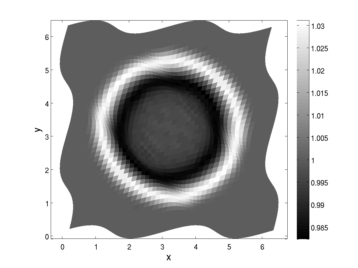
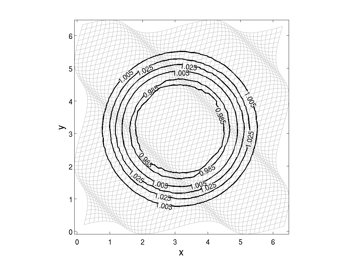
Figure 1: The density at T = 0.005s of an adiabatic pulse on a strongly distorted grid. Not that the correct interpolation of contour lines might add difficulties.

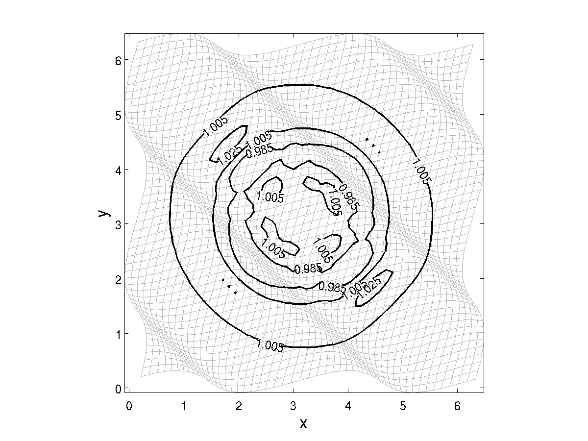
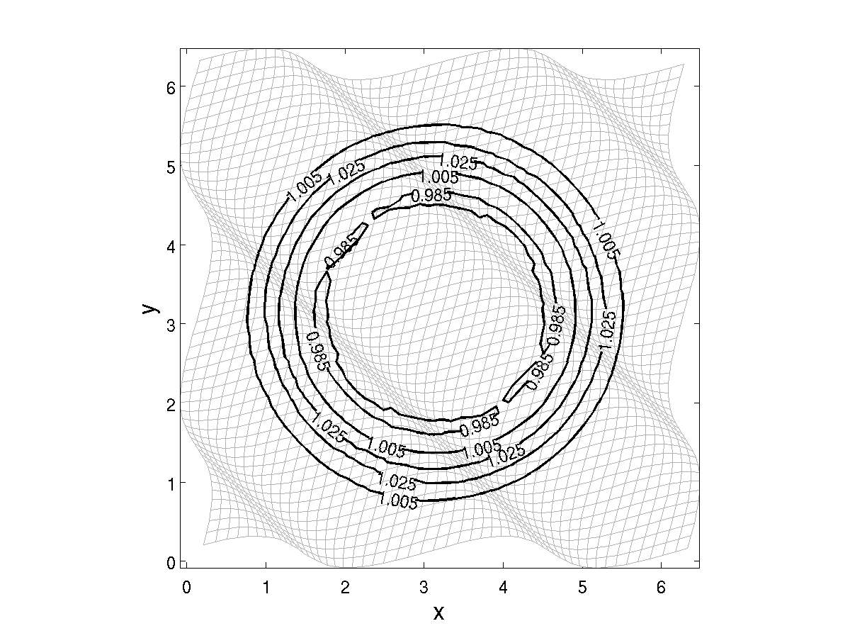
Figure 2: Selected contour lines of the density at T = 0.005s for a second order derivative and the Tam and Webb 4^th order derivative. The second order derivative has strong artefacts, while the TW derivative is much better.

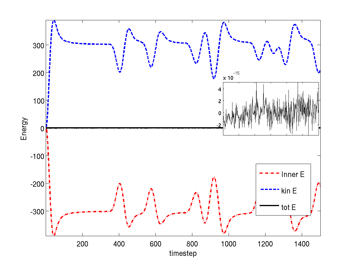
Figure 3: The conservation of the energy, calculated from mass, velocity and pressure. The change is at machine precision.

The same pressure pulse for a non-periodic grid with $k=1$ is presented in fig. 4; the boundaries are a slip wall and an non-reflecting boundary.

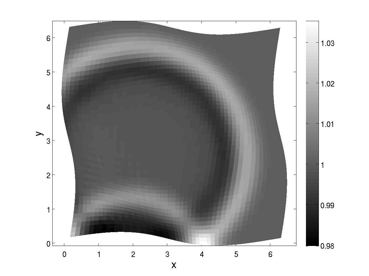
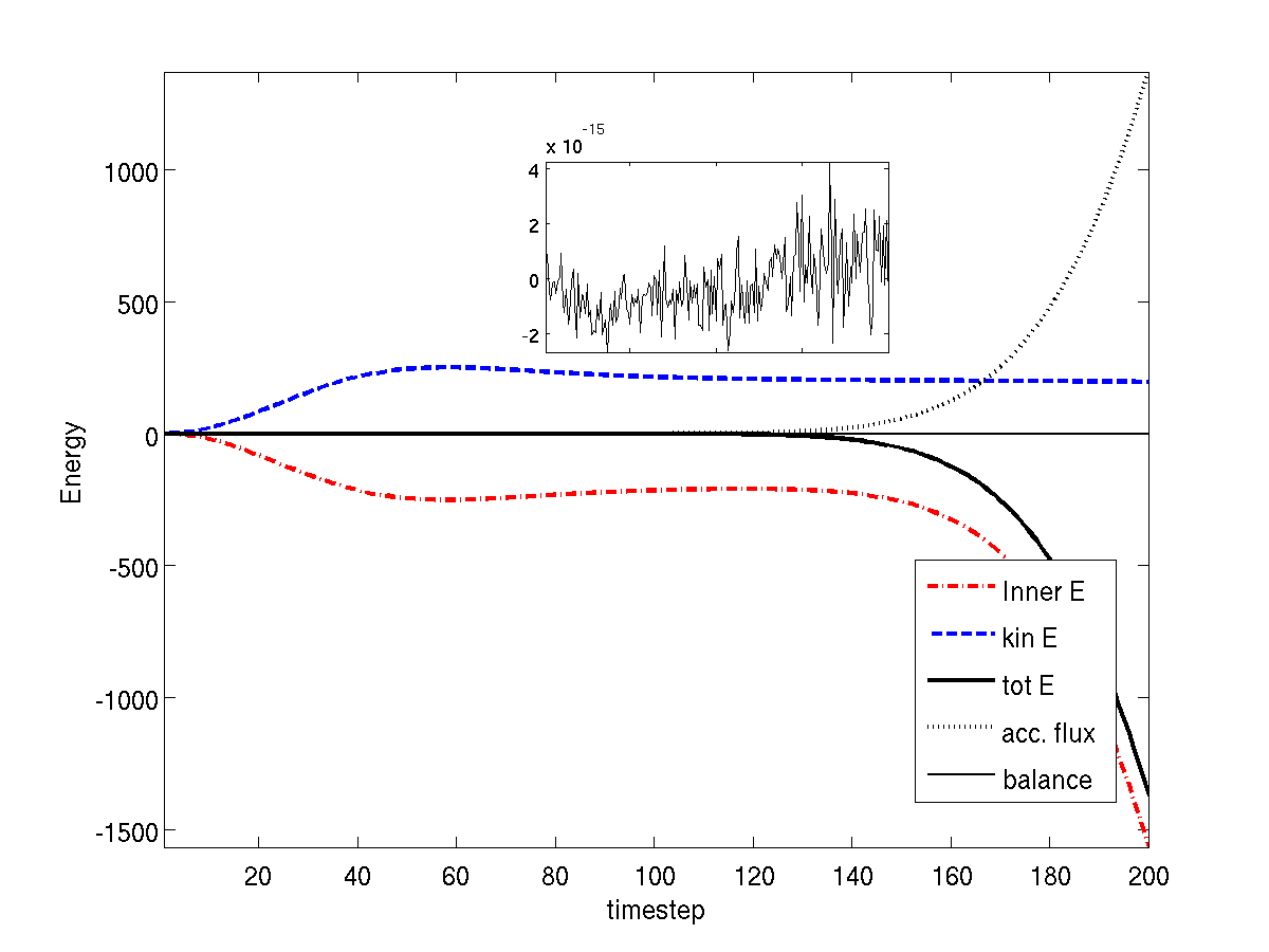
Figure 4: The density an adiabatic pulse on a non-periodic grid. Left: Accounting for the energy flux over the boundaries the energy is again conserved up to machine precision.

The boundaries conditions are calculated by a split in characteristic variables. The derivative is standard fourth order in the interior and reduces to a second order derivative described by Strand [16]. Fluxes are therefore calculated from boundary points only; enforcement of boundary conditions leads to a small extra term, which can uniquely be calculated by the difference between the calculated next time step without boundary conditions, compared with the values after setting the boundary conditions. Including the accumulated fluxes leads to a total conservation down to machine precision as in the periodic case.

6.2 Shock configuration

In the following we present a test case given by Lax and Liu [7]. Test case 13 was chosen, as shock and slip lines are present. We use no physical damping. As the scheme does not have numerical damping, we have to include a dissipation mechanism. This allows us to carefully add only the dissipation, which is needed on physical grounds, as in this example, demanded by shocks. A good way to do this is the adaptive and conservative filtering, presented by Bogey et al. [1], which depends on the divergence of the flow field. By this we introduce dissipation only where it is needed. This filtering is conservative when applied to conserved quantities, thus we filter the mass $\varrho$, the components of momentum $\varrho u_{\alpha}$ and the internal energy $p/(\gamma-1)$, which we increase by the change of kinetic energy to mimic a physical dissipation mechanism. By this we preserve the perfect conservation as before. The filtering is done after every time step. The adaptive filter can in principle create noise by changing the filter strength from time step to another. Even though this was not an issue in this test case, which proved to be very robust within our approach, we use a soft switching function for the filter strength $\sigma$ determined by the output of a shock detector $r$

$$\sigma=1-\mbox{tanh}((r_{th}/r)/\lambda).$$ (88)

instead of the more abrupt function used in [1]. A full description of the filter can be found in the given reference. The steepness of the switching function was $\lambda=2$ in the simulation, the threshold was $r_{th}=10^{-5}$. The initial values for $(\varrho,u,v,p)$ are (upper-right, upper-left, lower-left, lower-right) (1, 0, -0.3, 1), (2, 0, 0.3, 1), (1.0625, 0, 0.8145, 0.4) and (0.5313, 0, 0.4276, 0.4). As boundary conditions standard, non-reflecting boundary conditions are used, where the reference values are taken as the values in the neighbouring grid-points in the interior of the domain.

Figure 5: The density at t = 0.3 of the shock test case 13 of Lax and Liu [7]. Overall very good agreement is found, see discussion in the text for details.

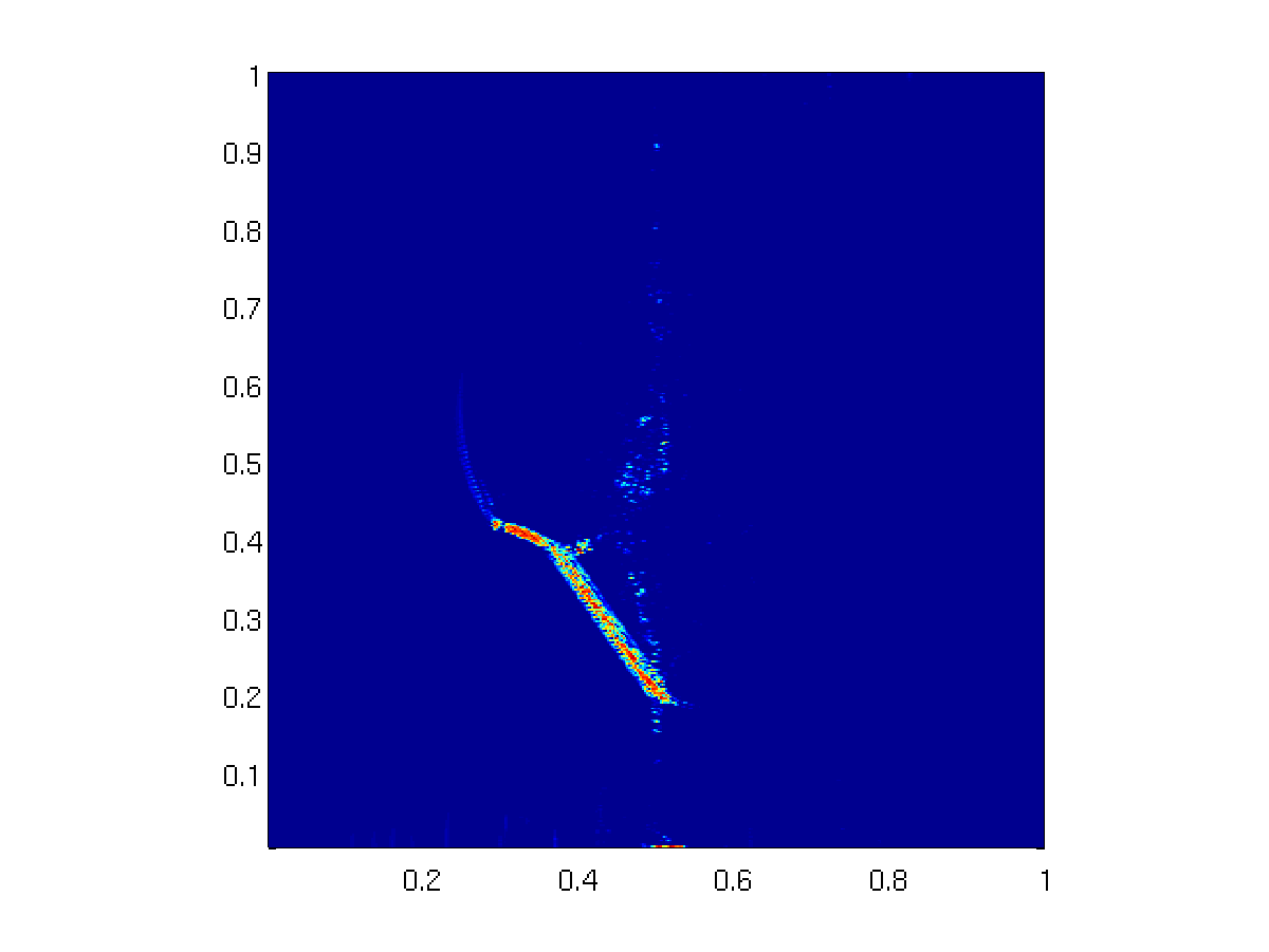
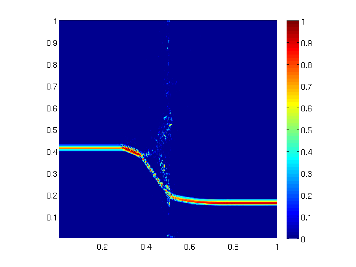
Figure 6: The adaptive shock filter strength $\sigma$ in x and y direction. It is apparent, that only at shocks the filter is involved whereas in other regions is is nearly zero.

Figure (5) shows excellent agreement of the density with the reference solution. The shock speeds agree with the reference case, as with the analytical formula; this is expected for a locally conservative code. For example the shock between upper-right and lower-right the shock speed is calculated as $s=[\varrho v^{2}+p]/[\varrho v]$ to be $s=-1.1246$, giving a shock location of $y=0.1626$. This is in perfect agreement with the simulation. To guarantee correct shock speeds, the scheme should have local and consistent fluxes. This issue is discussed for our FD scheme in B. However, three differences are visible. First the contour levels are not as smooth as in the original work; this is attributed to the fact that away from shocks absolutely no dissipation is involved. This could easily be smoothed by adding a small amount of physical or numerical dissipation, but it was left frictionless on purpose in this test case. Further the roll up in the center seems slightly different, and the slip line in the upper half is weakly wrinkled. The roll up was observed to depend sensitively on the chosen dissipation and might thus be hard to reproduce, as the implied friction in code used in [7] is difficult to estimate. The wrinkled slip line can be identified as the onset of a Kelvin-Helmholtz instability. This might be suppressed in [7] by the implied numerical damping. In contrast to the reference case, the dissipation in this simulation is the adaptive filter strength and is therefore known. It is shown in fig. (6), which shows that, whereas at shocks strong dissipation is found, the slip lines are only weakly filtered.

7 Conclusion

We presented a skew-symmetric finite difference scheme for fully compressible flows. It is strictly skew-symmetric and conservative also on distorted grids. The discrete form does purely build from point-wise operations and derivatives. This allows to use any explicit derivative which is skew-symmetric and has the telescoping sum property, in effect all derivatives with a symmetric stencil. By this any discretization order and wave-number optimized derivatives can directly be used. The implementation is simple and numerically efficient. Due to the described properties acoustics and shocks can be treated equally well. Boundary conditions and fluxes at the boundary can neatly be treated by summation by parts derivatives.

Appropriate time stepping schemes of high order and the use of standard time integrators are presented in a separate paper [5].

Appendix A Comparison with skew-symmetric schemes utilizing averaging

It is interesting to investigate, how this scheme compares with other skew-symmetric schemes, especially to the classical ansatz by Morinishi et al. [11], starting point for several other works on compressible and incompressible flows. Their discrete skew-symmetric momentum transport term, for second order accuracy, is in their notation, where we use Greek letters for the space index $2\cdot(Skew)=(Div)+(Adv)=\frac{\delta_{1}}{\delta_{1}x_{\beta}}\left({\overline{u}}^{1x_{\beta}}_{\beta}{\overline{u}}^{1x_{\beta}}_{\alpha}\right)+\overline{{\overline{u}}^{1x_{\beta}}_{\beta}\frac{\delta_{1}}{\delta_{1}x_{\beta}}{\overline{u}}^{1x_{\beta}}_{\alpha}}^{1x_{\beta}}$. The averaging operation is ${\overline{\phi}}^{nx_{\beta}}|_{\bf x}=\left(\phi|_{{\bf x}+\frac{n}{2}{\bf e}_{\beta}}+\phi|_{{\bf x}-\frac{n}{2}{\bf e}_{\beta}}\right)/2$ and the derivative is $\frac{\delta_{n}}{\delta_{n}x_{\beta}}\phi=\left(\phi|_{{\bf x}+\frac{n}{2}{\bf e}_{\beta}}-\phi|_{{\bf x}-\frac{n}{2}{\bf e}_{\beta}}\right)/(nh)$ with the unit grid vector ${\bf e}_{\beta}$ and the grid spacing $h$. A straight forward calculation reduces to the expression used by us (with $\varrho\equiv 1$):

$$2(Skew) = \frac{u_{\alpha,{\bf x}+{\bf e}_{\beta}}u_{\beta,{\bf x}+{\bf e}_{\beta}}-u_{\alpha,{\bf x}-{\bf e}_{\beta}}u_{\beta,{\bf x}-{\bf e}_{\beta}}}{2h}+u_{\beta,{\bf x}+{\bf e}_{\beta}}\frac{u_{\alpha,{\bf x}+{\bf e}_{\beta}}-u_{\alpha,{\bf x}-{\bf e}_{\beta}}}{2h}$$ (89)

$$= D_{x_{\beta}}(u_{\beta}u_{\alpha})-u_{\beta}D_{x_{\beta}}u_{\alpha}=(D_{x_{\beta}}U_{\beta}\cdot+U_{\beta}D_{x_{\beta}})u_{\alpha}$$

Choosing $\beta=1$ and $u_{\alpha}=u$ for the one dimensional case we arrive at our expression above. One should note, that the advective and the divergence term are different to ours due to the special averaging, and that only the combination are the same due to some cancellation and addition. A similar behaviour is expected for higher order derivatives. A generalization of this averaging procedure to the compressible case is presented by Kok [6]. The full scheme is expected to be different, as the other terms like mass flux are also constructed by averaging and no combination seems to reduce those to our form.

Our understanding is, that the spirit behind these works [11, 6] is to use averaging procedures to obtain a discrete version of the product rule, while we avoid to depend on this rule in the discrete by rewriting the equations analytically in a proper form.

Appendix B Defining Fluxes

When simulating shocks wrong shock speeds can be found even for consistent schemes [8]. The Lax-Wendroff theorem provides a set of conditions for which proper shocks are guaranteed. An essential condition for this theorem are local and consistent fluxes; a numerical flux is said to be local if it is calculated from a finite number of neighbouring discretization values; a numerical flux is consistent if it reduces to the analytical flux when this neighbouring discretization values are chosen to be constant. Being able to define consistent and local fluxes is therefore of central importance.

However, we stress , that the fluxes are not explicitly used in the implementation; it is a standard FD scheme building purely on derivative operations for means of simplicity and efficiency. The following part is thus only of theoretical importance.

We derive fluxes in one dimension for the sake of brevity; the derivation can be easily extended to more dimensions. We also work in time continuous case, as our goal are the spatial fluxes. A simple way to derive the fluxes is to split the sum over the full space occurring in the derivation of the global conservation into two parts, thus the derivation of the fluxes follows the proof of the conservations closely. This splitting written in the vector notation introduced earlier is ${\mathbf{1}}={\mathbf{l}}_{j+\frac{1}{2}}+{\mathbf{r}}_{j+\frac{1}{2}}$, where the $i^{th}$ component of vector ${\mathbf{r}}_{j+\frac{1}{2}}$ is given by

$${\mathbf{r}}_{j+\frac{1}{2}}=\left\{\begin{tabular}[]{ccl}$0$&\mbox{ for }&$i\leq j$\\ 1&\mbox{ for }&$i\geq j+1$\end{tabular}\right.,$$

and ${\mathbf{l}}_{j+1/2}$ accordingly with interchanged zeros and ones. The mass flux is derived from

$$-{\mathbf{1}}^{T}2\sqrt{\varrho}\partial_{t}\sqrt{\varrho}=-\partial_{t}{\mathbf{1}}^{T}\sqrt{\varrho}^{2}$$ (90)

$$= ({\mathbf{1}})^{T}D(\varrho u)=({\mathbf{l}}_{j+\frac{1}{2}}+{\mathbf{r}}_{j+\frac{1}{2}})^{T}D(\varrho u).$$

We are interested in the flux in the interior of the domain, we can thus assume zero fluxes at the domain-boundary and therefore conservation of mass. The telescoping sum property of the derivative therefore leads to

$$0=\underbrace{{\mathbf{l}}^{T}_{j+\frac{1}{2}}D(\varrho u)}_{f_{j+1/2}}+\underbrace{{\mathbf{r}}^{T}_{j+\frac{1}{2}}D(\varrho u)}_{f_{(j+1)-1/2}=-f_{j+1/2}}.$$ (91)

We can already conclude, first, that we can define fluxes and that secondly we have local fluxes, since we assume a finite stencil with constant coefficients. To prove the consistency of the fluxes we need information about the coefficients of the derivatives. Thus we calculate the weight coefficients $b_{j+\frac{1}{2}}$ of the the flux, given by

$${\mathbf{r}}^{T}_{j+\frac{1}{2}}D(\varrho u)=b_{j+\frac{1}{2}}^{T}(\varrho u).$$ (92)

The zeros in the definition of ${\mathbf{l}}_{j+\frac{1}{2}}$ remove the upper part $m\leq j$ of $D_{m,n}$, thus $b_{j+\frac{1}{2}}$ is given by

−a3−a2−a10a1a2a3⋱−a3−a2−a10a1a2a3⋱−a3−a2−a10a1a2⋱−a3⋱⋱)superscript1𝑇fragments missing-subexpressionfragmentsa3fragmentsa2fragmentsa10fragmentsa1fragmentsa2fragmentsa3missing-subexpressionmissing-subexpressionmissing-subexpression⋱fragmentsa3fragmentsa2fragmentsa10fragmentsa1fragmentsa2fragmentsa3missing-subexpressionmissing-subexpressionmissing-subexpression⋱fragmentsa3fragmentsa2fragmentsa10fragmentsa1fragmentsa2⋱missing-subexpressionmissing-subexpressionmissing-subexpressionmissing-subexpressionfragmentsa3⋱⋱missing-subexpressionmissing-subexpressionmissing-subexpression\displaystyle{\mathbf{1}}^{T}\left(\begin{tabular}[]{cccc|cccccc}\lx@intercol\hfil 0\hfil\lx@intercol &&\lx@intercol\hfil 0\hfil\lx@intercol \\ \hline\cr&$-a_{3}$&$-a_{2}$&$-a_{1}$&0&$a_{1}$&$a_{2}$&$a_{3}$\\ &$\ddots$&$-a_{3}$&$-a_{2}$&$-a_{1}$&$0$&$a_{1}$&$a_{2}$&$a_{3}$\\ &&$\ddots$&$-a_{3}$&$-a_{2}$&$-a_{1}$&$0$&$a_{1}$&$a_{2}$&$\ddots$\\ &&&&$-a_{3}$&$\ddots$&$\ddots$\\ \end{tabular}\right)

$$b_{j+\frac{1}{2}} = {\mathbf{1}}^{T}\left(\begin{tabular}[]{cccc|cccccc}\lx@intercol\hfil 0\hfil\lx@intercol &&\lx@intercol\hfil 0\hfil\lx@intercol \\ \hline\cr&$-a_{3}$&$-a_{2}$&$-a_{1}$&0&$a_{1}$&$a_{2}$&$a_{3}$\\ &$\ddots$&$-a_{3}$&$-a_{2}$&$-a_{1}$&$0$&$a_{1}$&$a_{2}$&$a_{3}$\\ &&$\ddots$&$-a_{3}$&$-a_{2}$&$-a_{1}$&$0$&$a_{1}$&$a_{2}$&$\ddots$\\ &&&&$-a_{3}$&$\ddots$&$\ddots$\\ \end{tabular}\right)$$ 0000 (98)

$$= ~{}~{}-(0,A_{n},\dots,A_{3},A_{2},A_{1},A_{1},A_{2},A_{3},\dots).$$ (99)

with $A_{k}=\sum_{i=k}^{n}a_{i}$. The finite stencil width is $n$. Note the symmetric structure of this coefficients. Therefore the mass flux is

$$f_{j+\frac{1}{2}}^{\varrho}=b_{j+\frac{1}{2}}^{T}(\varrho u)=\sum_{k=1}^{n}A_{k}\left((\varrho u)_{j+k}+(\varrho u)_{j-k+1}\right)$$ (100)

$$=\sum_{i=1}^{n}a_{i}\sum_{m=0}^{i-1}\left((\varrho u)_{j-m}+(\varrho u)_{j-m+i}\right).$$ (101)

The second form is gained by resorting the terms, also seen directly from the form of the matrix (99) . If we assume $(\varrho u)_{j+k}=const$ we get by summing of (100) simply by inspection of (99),

$$f_{j+\frac{1}{2}}^{\varrho}=b_{j+\frac{1}{2}}^{T}(\varrho u)=(\varrho u)\sum_{k=1}^{n}A_{k}=\varrho u\underbrace{2\sum\nolimits_{l}la_{l}}_{=1}=\varrho u.$$ (102)

The consistency condition of any numerical derivative enforces that the sum is unity.

The momentum flux is calculated from the combination of the mass and the momentum equation (${\mathbf{1}}^{T}[\ref{moriMom}+\frac{1}{2}U(\ref{moriMass})]$)

$${\mathbf{1}}^{T}\partial_{t}(u\sqrt{\varrho})\sqrt{\varrho}\\ +{\mathbf{1}}^{T}D^{\varrho u}u+{\mathbf{1}}^{T}Dp\\ +\frac{1}{2}{\mathbf{1}}^{T}U(DU\varrho)=0.$$

Most terms in the momentum equation are in divergence form and can reduce to fluxes as before. Splitting the sum ${\mathbf{1}}={\mathbf{l}}_{j+\frac{1}{2}}+{\mathbf{r}}_{j+\frac{1}{2}}$ and assuming zero flux over the boundaries we obtain

$$f^{\varrho u}_{j+\frac{1}{2}}=b_{j+\frac{1}{2}}^{T}\left(\frac{1}{2}({u}\varrho)u+p\right)+\frac{1}{2}{\mathbf{r}}^{T}_{j+\frac{1}{2}}U[DU\varrho+RDu].$$ (103)

The remaining term of the non-linear transport combines with the term in of the mass equation the last term is found to be

$${\mathbf{r}}^{T}_{j+\frac{1}{2}}U[DU\varrho+RDu]=u^{T}\underbrace{\left[({\mathbf{r}}_{j+\frac{1}{2}}D)^{T}+({\mathbf{r}}_{j+\frac{1}{2}}D)\right]}_{B}({u}\varrho),$$ (104)

where the matrix $B_{m,n}$ has zero block for $m,n\leq j$ and $j+1\geq m,n$ :

−a2−a3⋱−a1−a2−a3−a3−a2−a1⋱−a3−a2⋱−a3),fragments missing-subexpressionmissing-subexpressionmissing-subexpressionfragmentsa2fragmentsa3⋱missing-subexpressionmissing-subexpressionmissing-subexpressionmissing-subexpressionfragmentsa1fragmentsa2fragmentsa3missing-subexpressionfragmentsa3fragmentsa2fragmentsa1missing-subexpressionmissing-subexpressionmissing-subexpressionmissing-subexpression⋱fragmentsa3fragmentsa2missing-subexpressionmissing-subexpressionmissing-subexpressionmissing-subexpressionmissing-subexpression⋱fragmentsa3missing-subexpressionmissing-subexpressionmissing-subexpressionmissing-subexpression\displaystyle\left(\begin{tabular}[]{cccc|cccccc}&&&&$-a_{3}$&$\ddots$&$$\\ &&&&$-a_{2}$&$-a_{3}$&$\ddots$\\ &&&&$-a_{1}$&$-a_{2}$&$-a_{3}$\\ \hline\cr&$-a_{3}$&$-a_{2}$&$-a_{1}$&&&&\\ &$\ddots$&$-a_{3}$&$-a_{2}$&&&\\ &&$\ddots$&$-a_{3}$&\end{tabular}\right),

$$B = \left(\begin{tabular}[]{cccc|cccccc}&&&&$-a_{3}$&$\ddots$&$$\\ &&&&$-a_{2}$&$-a_{3}$&$\ddots$\\ &&&&$-a_{1}$&$-a_{2}$&$-a_{3}$\\ \hline\cr&$-a_{3}$&$-a_{2}$&$-a_{1}$&&&&\\ &$\ddots$&$-a_{3}$&$-a_{2}$&&&\\ &&$\ddots$&$-a_{3}$&\end{tabular}\right),$$ -a3⋱-a3⋱ (111)

so that

$$u^{T}{B}({u}\varrho) = \sum_{i=1}^{n}a_{i}\sum_{m=0}^{i-1}\left(u_{j-m+i}(\varrho u)_{j-m}+u_{j-m}(\varrho u)_{j-m+i}\right).$$

Again by inspection or summing it is easy to see that this numerical flux reduces to the analytical flux $u(\varrho u)$ provided we use a consistent derivative.

Altogether we obtain

$$f^{\varrho u}_{j+\frac{1}{2}}=b_{j+\frac{1}{2}}^{T}\left(\frac{1}{2}({u}\varrho u)+p\right)+\frac{1}{2}u^{T}{B}({u}\varrho),$$

where $\varrho,u,p$ are the vectors of the discretization values.

The momentum flux by the non-linear transport is therefore

$$u^{T}{B}({u}\varrho)+b_{j+\frac{1}{2}}^{T}\frac{1}{2}({u}\varrho u)$$ (112)

$$= \sum_{i=1}^{n}a_{i}\sum_{m=0}^{i-1}\left((\varrho uu)_{j-m}+(\varrho uu)_{j-m+i}\right)+\sum_{i=1}^{n}a_{i}\sum_{m=0}^{i-1}\left(u_{j-m+i}(\varrho u)_{j-m}+u_{j-m}(\varrho u)_{j-m+i}\right)$$

$$= \sum_{i=1}^{n}a_{i}\sum_{m=0}^{i-1}\left[u_{j-m+i}+u_{j-m}\right]\left[(\varrho u)_{j-m+i}+(\varrho u)_{j-m}\right],$$

which is just the same as in [14], which is not by chance. In the derivation of the momentum flux the momentum and the mass equation had to be combined, which leads to exactly the same spatial terms as in the flux splitting approach. Of course differences in the two schemes arise when the energy equation is not split in the kinetic and internal energy parts, as it is apparently the case, and of course for the time discrete case, as a standard time integration scheme is used.

The flux of the total energy is derived as ${\mathbf{1}}^{T}(\ref{moriEn})$ , where $UDp$ is replaced with the help of (54)

$$0 = \partial_{t}{\mathbf{1}}^{T}p~{}\phantom{(+\frac{u^{2}}{2})}+\frac{\gamma}{\gamma-1}{\mathbf{1}}^{T}DUp-{\mathbf{1}}^{T}UDp$$ (113)

$$= \partial_{t}{\mathbf{1}}^{T}(p+\frac{u^{2}}{2})+\frac{\gamma}{\gamma-1}{\mathbf{1}}^{T}DUp+{\mathbf{1}}^{T}UD^{\varrho u}u,$$ (114)

and splitting the sum, ${\mathbf{1}}={\mathbf{l}}_{j+\frac{1}{2}}+{\mathbf{r}}_{j+\frac{1}{2}}$, as before. The flux in the inner energy $e=p/(\gamma-1)$ is analogous to the flux of the mass. The flux form the coupling to the kinetic energy

$${\mathbf{r}}^{T}_{j+\frac{1}{2}}UD^{\varrho u}u=u^{T}\tilde{D}^{\varrho u}u$$

with $\tilde{D}^{\varrho u}=\tilde{D}UR+RU\tilde{D}$, where $\tilde{D}_{m,n}$ is the derivative matrix, with the lines $m\leq j$ is set to zero. The value of a quadratic forms is given by the symmetric part of the matrix, here

$$\frac{(\tilde{D}^{\varrho u})+(\tilde{D}^{\varrho u})^{T}}{2}=\frac{1}{2}\left(BUR+RUB\right)$$ (115)

with $B$ as before. Thus the flux is

$$f^{e}_{j+\frac{1}{2}}=\frac{\gamma}{\gamma-1}b_{{\mathbf{r}},j+\frac{1}{2}}^{T}(pu)+\frac{1}{2}u^{T}\left(BUR+RUB\right)u.$$

By the same arguments as before the flux is local and consistent.

The derivation of fluxes for the three dimensional case on transformed grids are in principle calculated in the same manner, but the derivation is much more cumbersome. The Jacobian is multiplied to the conserved quantities, as expected. The geometrical factors for the conservative form are just multiplied. The geometrical factors for the non-conservative forms enter in the quadratic forms and can be absorbed in the weight factors.

References

• [1] Ch. Bogey, N. de Cacqueray, and Ch. Bailly. A shock-capturing methodology based on adaptative spatial filtering for high-order non-linear computations. J. Comp. Phys., 228(5):1447 – 1465, 2009.
• [2] Mark H. Carpenter, David Gottlieb, and Saul Abarbanel. Time-stable boundary conditions for finite-difference schemes solving hyperbolic systems: Methodology and application to high-order compact schemes. Journal of Computational Physics, 111(2):220 – 236, 1994.
• [3] F. Ducros, F. Laporte, T. Soulères, V. Guinot, P. Moinat, and B. Caruelle. High-order fluxes for conservative skew-symmetric-like schemes in structured meshes: Application to compressible flows. Journal of Computational Physics, 161(1):114 – 139, 2000.
• [4] Gregor J Gassner. A skew-symmetric discontinuous galerkin spectral element discretization and its relation to sbp-sat finite difference methods. SIAM Journal on Scientific Computing, 35(3):A1233–A1253, 2013.
• [5] Jörn Sesterhenn Jens Brouwer, Julius Reiss. Conservative time integrators of arbitrary order for skew-symmetric finite-difference discretizations of compressible flow. Computers & Fluids, submitted:xxx, 2013.
• [6] J.C. Kok. A high-order low-dispersion symmetry-preserving finite-volume method for compressible flow on curvilinear grids. Journal of Computational Physics, 228(18):6811 – 6832, 2009.
• [7] Peter D. Lax and Xu-Dong Liu. Solution of two-dimensional riemann problems of gas dynamics by positive schemes. SIAM J. Sci. Comput., 19(2):319–340, March 1998.
• [8] Randall J. LeVeque. Numerical methods for conservation laws. Lectures in Mathematics. Birkhäuser-Verlag, Basel, 1992.
• [9] Y. Morinishi. Skew-symmetric form of convective terms and fully conservative finite difference schemes for variable density low-mach number flows. JCP, 229(2):276–300, 2010.
• [10] Y. Morinishi and K. Koga. Skew-symmetric convection form and secondary conservative finite difference methods for moving grids. Journal of Comp. Phys., in press:xxx, 2013.
• [11] Y. Morinishi, T.S. Lund, O.V. Vasilyev, and P. Moin. Fully conservative higher order finite difference schemes for incompressible flow. Journal of Computational Physics, 143(1):90 – 124, 1998.
• [12] Youhei Morinishi. Forms of convecction and quadratic conservative finite difference schemes for low mach number compressible flow simulations. Trans. Jap. Soc. Mech. Engin. B, pages 451–458, 2007.
• [13] Pelle Olsson. Summation by parts, projections, and stability. RICAS Tech. Rep. 93.04, 1993.
• [14] Sergio Pirozzoli. Generalized conservative approximations of split convective derivative operators. Journal of Computational Physics, 229(19):7180 – 7190, 2010.
• [15] Julius Reiss and Jörn Sesterhenn. Conservative, skew–symmetric discretization of the compressible navier– stokes equations. In Andreas Dillmann, Gerd Heller, Hans-Peter Kreplin, Wolfgang Nitsche, and Inken Peltzer, editors, New Results in Numerical and Experimental Fluid Mechanics VIII, volume 121 of Notes on Numerical Fluid Mechanics and Multidisciplinary Design, pages 395–402. Springer Berlin Heidelberg, 2013.
• [16] Bo Strand. Summation by parts for finite difference approximations for d/dx. Journal of Computational Physics, 110(1):47 – 67, 1994.
• [17] Pramod K. Subbareddy and Graham V. Candler. A fully discrete, kinetic energy consistent finite-volume scheme for compressible flows. Journal of Computational Physics, 228(5):1347 – 1364, 2009.
• [18] Joe F. Thompson. Numerical Grid Generation. Elsevier, Amsterdam, 1985.
• [19] R. W. C. P. Verstappen and A. E. P. Veldman. Symmetry-preserving discretization of turbulent flow. JCP, 187(1):343, 2003.