Habilitation à diriger des recherches

 Mémoire présenté par Nicolas Trotignon
 CNRS, LIAFA, Université Paris 7, Paris Diderot

 Structure des classes de graphes définies
 par l’exclusion de sous-graphes induits

Résumé — Abstract

Ce document présente les recherches de l’auteur durant ces dix dernieres années, sur les classes de graphes définies en excluant des sous-graphes induits.

This document presents the work of the author over the last ten years on classes of graphs defined by forbidding induced subgraphs.

Remerciements

Je remercie Maria Chudnovsky, Michele Conforti et Stéphan Thomassé d’avoir accepté d’être les rapporteurs externes de ce travail. Merci également aux autres membres du jury : Jean-Paul Delahaye, Michel Habib et Frédéric Maffray.

Merci à Christelle Petit, Jean-Sébastien Sereni et Rachel Wieviorka qui m’ont aidé à améliorer ce document. Merci surtout à Juraj Stacho et Béatrice Trotignon qui en ont relu de nombreuses pages.

Merci à mon épouse Christelle et à mes enfants Émile, Alice et Coline pour leur soutien et leur affection.

Contents

1. Introduction (en français)
   1. Plan du document
   2. Section 2.6 traduite en français
2. Introduction (in English)
   1. Outline of the document
   2. How to read this document
   3. Perfect graphs
3. 1 Mind the gap
   1. 1.1 Basic facts about the gap
   2. 1.2 Ramsey Theory and asymptotic results
   3. 1.3 Triangle-free gap-critical graphs
   4. 1.4 Small gap-extremal graphs
   5. 1.5 Conclusion
4. 2 Six simple decomposition theorems
   1. 2.1 Subdivisions of a paw
   2. 2.2 Triangle and $T_{123}$
   3. 2.3 Chordless graphs
   4. 2.4 Line-graphs of triangle-free graphs
   5. 2.5 Claw and coclaw
   6. 2.6 Weakly triangulated graphs
5. 3 Detecting induced subgraphs
   1. 3.1 A tool for NP-completeness: Bienstock’s Construction
   2. 3.2 A tool for polynomiality (1): shortest path detectors
   3. 3.3 A tool for polynomiality (2): three-in-a-tree
   4. 3.4 Generalizing three-in-a-tree
6. 4 Two decomposition theorems
   1. 4.1 Cycles with a unique chord
   2. 4.2 Induced subdivision of $K_{4}$
   3. 4.3 Graphs with no wheels
7. 5 Berge graphs
   1. 5.1 Decomposing Berge graphs: main results
   2. 5.2 Detection of balanced skew partitions
   3. 5.3 A new decomposition theorem for Berge graphs
   4. 5.4 Decomposing Berge graphs with no skew partitions and no homogeneous pairs
      1. 5.5 Cliques and stable sets in Berge graphs with no skew partitions and no homogeneous pairs
         1. 5.6 Coloring Berge graphs using subroutines for cliques and stable sets
            1. 5.7 A bit of science-fiction: coloring Berge graphs
               1. A Curriculum vitæ
               2. B Activités d’encadrement
               3. C Résumé sur l’originalité des recherches
               4. D Exposé synthétique des recherches
               5. E Perspectives
               6. F Liste des travaux
               7. Bibliography

Introduction (en français)

Ce document présente mon travail de ces dix dernières années en théorie des graphes. Le premier chapitre expose une étude sur le “gap” d’un graphe, c’est-à-dire l’écart entre la taille d’une plus grande de ses cliques et son nombre chromatique. C’est l’occasion d’introduire des notions importantes pour le reste du document, en particulier la notion de fonction majorante (bounding function) due initialement à András Gyárfás. Ce chapitre utilise des outils de plusieurs branches de la théorie des graphes, comme la théorie de Ramsey et celle des couplages. J’espère que ce chapitre divertira tout ceux qui apprécient la théorie des graphes, peut-être même ceux qui ne l’apprécient pas.

Le reste du document se concentre sur ce que je fais ordinairement, à savoir étudier des classes de graphes définies par l’exclusion de certains sous-graphes induits, donner des théorèmes de décomposition et des algorithmes pour ces classes. Pourquoi exclure des sous-graphes induits ? Essayons de donner une réponse meilleure que “parce qu’il y a 10 ans, mon directeur de thèse, Frédéric Maffray, m’a dit de le faire” ou “parce que il y a beaucoup des sous-graphes induits possibles, ce qui conduira à publier beaucoup d’articles”. Notons tout d’abord que tout classe fermée pour la relation “sous-graphe induit” est nécessairement définie de manière équivalente par une liste de sous-graphes induits exclus. Et cette relation “sous-graphe induit” est mathématiquement “naturelle” en ce qu’elle correspond à la notion classique de “sous-structure” présente partout en algèbre et dans toutes les branches des mathématiques. De plus, dans plusieurs modèles de Recherche Opérationnelle, des problèmes pratiques sont modélisés par des graphes. Les objets considérés sont les sommets du graphe tandis que les contraintes entre objets sont représentées par les arêtes. Souvent, la classe de graphes résultant d’une telle modélisation est fermée par sous-graphes induits. Car supprimer des objets dans le monde réel correspond à supprimer des sommets du graphes, tandis que supprimer des contraintes entre objets ne correspond à aucune opération du monde réel ; de telle sorte que toutes les arêtes qui existent entre les sommets non-suprimés du graphe doivent demeurer.

Dans les années 1960, le travail pionnier de Gabriel Dirac sur les graphes chordaux, de Tibor Gallai sur les graphes de comparabilité et les deux conjectures des graphes parfaits de Claude Berge ont inauguré le domaine. Au long des quarante années qui ont suivi, beaucoup de recherches ont été consacrées aux graphes parfaits et à d’autres classes des graphes, avec de nombreux succès, comme la preuve de la conjecture faible des graphes parfaits par Laszlo Lovász, les résultats de Vašek Chvátal et Delbert Fulkerson sur le lien entre les graphes parfaits et la programmation linéaire, et la preuve de la conjecture forte des graphes parfaits par Maria Chudnovsky, Neil Robertson, Paul Seymour et Robin Thomas.

À partir des années 1980, Neil Robertson et Paul Seymour ont développé le “Graph Minor Project”. Il s’agit d’une théorie très profonde qui décrit toutes les classes de graphes fermées pour la relation de mineur (et non pas de sous-graphe induit). Il est naturel de se demander si une telle théorie pourrait exister pour la relation de sous-graphe induit. Jusqu’à présent, il semblerait que la réponse soit négative. Les classes fermées pour la relation de sous-graphe induit ne semblent pas assez régulières pour être décrites par une théorie unifiée. Un indice parmi d’autres est donné au chapitre 3 de ce travail, où plusieurs classes de graphes sont poynomiales ou NP-complètes à reconnaître, en fonction de changements apparemment insignifiants dans leur définition. Pourtant, il pourrait y avoir des caractéristiques partagées par toutes les classes de graphes définies en interdisant un sous-graphe induit (voir par exemple la conjecture de Erdős-Hajnal), ou par beaucoup de classes définies plus généralement (voir par exemple la conjecture de Gyárfás sur les arbres, Conjecture 2.7, ou la conjecture de Scott, Conjecture 2.3). La question qui m’intéresse le plus est de comprendre comment les classes de graphes fermées par sous-graphes induits peuvent être décrites de la manière la plus générale possible. Mais comme le lecteur le constatera, la plupart des résultats présentés ici concerne des classes particulières.

Plan du document

Rappelons que le chapitre 1 présente des résultats à propos de l’écart entre le nombre chromatique et la taille d’une plus grande clique d’un graphe. Ce chapitre s’inspire de [50].

L’outil le plus puissant ces dernières années pour l’étude des classes fermées par sous-graphe induit est l’approche structurelle, qui consiste en la description des classes de graphes à travers des théorèmes de décomposition. Ceci est expliqué au chapitre 2 où six théorèmes de décomposition sont présentés. Ces théorèmes sont tous assez simples, mais la motivation de ce chapitre est de présenter un échantillon typique de théorie structurelle des graphes à destination de lecteurs ne voulant pas se lancer dans la lecture d’articles ou d’analyses de cas trop longs. Les preuves sont toutes assez courtes, mais elles tentent d’illustrer des idées qui seront utilisées dans le reste du document. Ce chapitre peut aussi être utilisé pour enseigner la théorie structurelle des graphes. Ce chapitre ne s’inspire pas d’un article particulier, il reprend des théorèmes divers, donne parfois des nouvelles preuves, et aussi quelques résultats originaux.

Le chapitre 3 présente un aspect important des classes de graphes définies par sous-graphes induits exclus. Comment décider avec un algorithme si tel graphe est dans telle classe ? L’approche la plus simple semble de voir comment on peut détecter des sous-graphes induits dans un graphe donné. Nous montrerons que certains problèmes de ce type sont polynomiaux, d’autres NP-complets. Les outils pour la NP-complétude proviennent tous d’une construction de Bienstock. L’outil le plus général pour montrer la polynomialité semble être l’algorithme dit “three-in-a-tree” dû à Chudnovsky et Seymour. Nous donnerons des variantes de cet algorithme. Ce chapitre s’inspire de [68], [78], [71] et [37].

Le chapitre 4 est consacré à deux classes de graphes : les graphes qui ne contiennent pas de cycle avec une seule corde, et les graphes qui ne contiennent pas de subdivision induite de $K_{4}$. La motiviation initiale pour l’étude de ces classes était leur reconnaissance en temps polynomial, un problème issu du chapitre précédant. Mais leur étude nous a conduit à des résultats sur le nombre chromatique. Ce chapitre s’inspire de [105] et [69].

Le chapitre 5 est consacré aux graphes de Berge. On procède d’abord à un survol des résultats importants concernant leur structure. Nous donnons un théorème de structure pour les graphes de Berge sans partition antisymétrique paire (balanced skew partition). Comme application de ce théorème, nous donnons un algorithme de coloration des graphes de Berge sans partition antisymétrique paire et sans paire homogène. Ce chapitre s’inspire de [104] et [106].

Les annexes A à F présentent des données obligatoires pour tout mémoire d’habilitation. L’annexe F donne la liste de mes publications et indique où trouver dans ce mémoire le contenu de tel ou tel article.

La plupart des travaux présentés ci-après ont été réalisés en collaboration. Les contributions de chacun seront précisées au fur et à mesure, mais je suis heureux de donner maintenant la liste de mes co-auteurs : Amine Abdelkader, Nicolas Dehry, Sylvain Gravier, András Gyárfás, Benjamin Lévêque, David Lin, Christophe Picouleau, Jérôme Renault, András Sebő, Juraj Stacho et Liu Wei. Je voudrais remercier plus particulièrement deux co-auteurs avec qui mes collaborations ont été très proches et enrichissantes : Frédéric Maffray et Kristina Vušković.

Le lecteur francophone qui a fait l’effort de me lire jusqu’ici, constatera s’il poursuit que ce travail a été rédigé en anglais, ce qui le situe à la marge de la légalité. Avec le conseil scientifique de mon UFR, il a été convenu qu’une dizaine de pages en français devrait suffir et constituer officiellement mon mémoire, le reste étant une “annexe”. Ne pouvant pas raisonnablement faire passer ce qui précède pour une “dizaine”, ni même pour une “petite” dizaine de pages, je me propose de donner ci-dessous la traduction de la section de ce document dont la lecture est la plus profitable selon moi, la section 2.6. On a d’abord besoin de quelques rappels.

Rappels

Un trou dans un graphe est un cycle induit de longueur au moins 4. Un antitrou est un trou du graphe complémentaire. Un graphe de Berge est un graphe qui ne contient ni trou impair ni antitrou impair. Notons qu’on utilise le mot contenir au sens des sous-graphes induits. Une clique est un graphe dont tous les sommets sont reliés (deux à deux). Par $\chi(G)$ on dénote le nombre chromatique de $G$, par $\omega(G)$ le plus grand nombre de sommets deux à deux adjacents de $G$. Claude Berge a conjecturé au début des années soixante que tout graphe de Berge $G$ satisfait ce qu’il appelait la belle propriété : $\chi(G)=\omega(G)$. Ceci est devenu la célèbre conjecture forte des graphes parfaits, prouvée par Chudnovsky, Robertson, Seymour et Thomas en 2002. Il est facile de voir que les trous impairs et les antitrous impairs ne satisfont pas la belle propriété, mais cette remarque n’aide pas tellement à montrer la conjecture… Un trou ou un antitrou est long s’il contient au moins 5 sommets. Un graphe est dit parfait si pour tout sous-graphe induit $G^{\prime}$ on a $\chi(G^{\prime})=\omega(G^{\prime})$.

Le théorème de décomposition le plus simple pour une classe de graphes est sans doute le suivant.

Théorème 0.1 (folklore)

Un graphe ne contient aucun $P_{3}$ induit si et seulement si c’est une union disjointe de cliques.

preuve — Une union disjointe de cliques est manifestement sans $P_{3}$. Réciproquement, considérons une composante connexe $C$ d’un graphe sans $P_{3}$ et supposons en vue d’une contradiction que deux sommets $u,v$ de $C$ ne sont pas adjacents. Un plus court chemin de $C$ joignant $u$ à $v$ contient un $P_{3}$, contradiction (ou comme eût dit Claude Berge, d’où l’absurdité). $\Box$

Section 2.6 traduite en français

Un graphe est faiblement triangulé s’il ne contient ni trou long ni antitrou long. Les graphes faiblement triangulés sont donc de Berge, et nous allons montrer qu’ils satisfont la belle propriété, ce qui prouve leur perfection et donne une version affaiblie du théorème fort des graphes parfaits. Les graphes faiblement triangulés ont été étudiés par Chvátal et Hayward dans les années 1980 et le but de cette section est de convaincre le lecteur qu’ils constituent l’une des classes de graphes de Berge les plus intéressantes. Car avec eux, on peut comprendre plusieurs concepts en lisant seulement six pages : les lemmes du type Roussel-et-Rubio, comment traiter les antitrous, comment des décompositions désagréables comme les partitions antisymétriques (skew partitions) entrent en jeux, en quoi elle sont désagréables, comment on peut parfois s’en débarrasser grâce à des sommets spéciaux (les paires d’amis, en anglais “even pairs”) et obtenir des algorithmes de coloration simples et efficaces.

Le lemme de Roussel et Rubio [96] est un outil technique important pour la preuve du théorème fort des graphes parfaits. L’équipe qui a prouvé ce théorème a redécouvert le lemme indépendamment de ses auteurs et l’a baptisé le “wonderful lemma” en raison de ses nombreuses applications. Il dit qu’en un sens, tout ensemble anticonnexe de sommets d’un graphe de Berge se comporte comme un sommet (anticonnexe signifie connexe dans le complémentaire). Comment un sommet se “comporte”-t-il dans un graphe de Berge ? Si un chemin de longueur impaire (au moins 3) a ses deux extrémités adjacentes à $v$, alors $v$ doit avoir d’autres voisins dans le chemin car sinon il y a un trou impair. Un ensemble anticonnexe $T$ de sommets se comporte de la même manière : si un chemin de longueur impaire (au moins 3) a ses deux extrémités complètes à $T$, alors au moins un sommet intérieur du chemin doit aussi être complet à $T$. En fait, il y a deux exceptions à cet énoncé et le lemme de Roussel et Rubio est un peu plus compliqué. Nous ne donnons pas ici son énoncé exact. Pour plus d’informations, variantes et preuves courtes notamment, voir le Chapitre 4 de [103].

Voici un lemme qui peut être vu comme une version du lemme de Roussel et Rubio [96] pour les graphes faiblement triangulés.

Lemme 0.2 (avec Maffray [79])

Soit $G$ un graphe faiblement triangulé. Soit $P=x\!-\!\cdots\!-\!y$ un chemin de $G$ de longueur au moins 3 et $T\subseteq V(G)$, disjoint de $V(P)$ et tel que $G[T]$ soit anticonnexe, et les extrémités de $P$ sont $T$-complètes. Alors $P$ contient un sommet intérieur qui est $T$-complet.

preuve — Noter qu’aucun sommet $t\in T$ peut être non-adjacent à deux sommets consécutifs de $P$ car alors $V(P)\cup\{t\}$ contient un trou long. Soit $z$ un sommet intérieur de $P$ adjacent à un nombre maximum de sommets de $T$. Supposons, en vue d’une contradiction, qu’il existe un sommet $u\in T\setminus N(z)$. Soient $x^{\prime}$ et $y^{\prime}$ les voisins de $z$ sur $P$, nommés de sorte que $x,x^{\prime},z,y^{\prime},y$ apparaissent dans cet ordre le long de $P$. Alors, d’après la première phrase de cette preuve, $ux^{\prime},uy^{\prime}\in E(G)$. À un renommage près de $x$ et $y$, on suppose que $x^{\prime}\neq x$. D’après le choix de $z$, puisque $ux^{\prime}\in E(G)$ et $uz\notin E(G)$, il existe un sommet $v\in T$ tel que $vz\in E(G)$ et $vx^{\prime}\notin E(G)$. Puisque $G[T]$ est anticonnexe, il existe un antichemin $Q$ de $G[T]$ de $u$ vers $v$, et $u,v$ sont choisis pour que cet antichemin soit minimal. D’après la première phrase de cette preuve, les sommets intérieurs de $Q$ sont tous adjacents à $x^{\prime}$ ou $z$ et d’après la minimalité de $Q$, les sommets intérieurs de $Q$ sont tous adjacents à $x^{\prime}$ et $z$. Si $x^{\prime}x\notin E(G)$ alors $V(Q)\cup\{x,x^{\prime},z\}$ induit un antitrou long. Donc $x^{\prime}x\in E(G)$. Si $zy\notin E(G)$ alors $V(Q)\cup\{z,x^{\prime},y\}$ induit un antitrou long. Donc $zy\in E(G)$ et $y=y^{\prime}$. Mais alors, $V(Q)\cup\{x,x^{\prime},z,y\}$ induit un antitrou long, une contradiction. $\Box$

Quand $T$ est un ensemble de sommets, $C(T)$ dénote l’ensemble des sommets complets à $T$.

Lemma 0.3

Soit $G$ un graphe faiblement triangulé et $T$ un ensemble de sommets tel que $G[T]$ est anticonnexe et $C(T)$ contient au moins deux sommets non adjacents. Supposons que $T$ soit maximal au sens de l’inclusion avec ces propriétés. Alors tout chemin de $G\setminus T$ dont les extrémités sont dans $C(T)$ a tous ses sommets dans $C(T)$.

preuve — Soit $P$ un chemin de $G\setminus T$ dont les extrémité sont dans $C(T)$. Si un sommet de $P$ n’est pas dans $C(T)$, alors $P$ contient un sous-chemin $P^{\prime}$ de longueur au moins 2 dont les extrémités sont dans $C(T)$ et dont l’intérieur est disjoint de $C(T)$. Si $P^{\prime}$ est de longueur 2, soit $P^{\prime}=a\!-\!t\!-\!b$, alors $T\cup\{t\}$ est ensemble qui contredit la maximalité de $T$. Si $P^{\prime}$ est de longueur supérieure à 2, alors il contredit le lemme 0.2. $\Box$

Le théorème suivant est dû à Hayward, mais j’en propose ici une nouvelle preuve. Ma preuve n’est pas vraiment plus courte que celle de Hayward, mais elle montre comment des lemmes du type Roussel et Rubio peuvent être utilisés. Un ensemble d’articulation d’un graphe est un ensemble $S$ de sommets tel que $G\setminus S$ n’est pas connexe. Une étoile d’un graphe est un ensemble de sommets $S$ qui contient un sommet $c$ tel que $S\subseteq N[c]$. Une étoile d’articulation est une étoile qui est un ensemble d’articulation.

Théorème 0.4 (Hayward [54])

Soit $G$ un graphe faiblement triangulé. Alors ou bien :

• $G$ est une clique;

• $G$ est le complémentaire d’un couplage parfait;

• $G$ possède une étoile d’articulation.

preuve — Si $G$ est une union disjointe de cliques, en particulier quand $|V(G)|\leq 2$, alors la conclusion du théorème est satisfaite. D’après le théoreme 0.1, on peut donc supposer que $G$ contient un $P_{3}$. Donc, il existe un ensemble $T$ de sommets tel que $G[T]$ est anticonnexe et $C(T)$ contient au moins deux sommets non-adjacents, parce que le milieu d’un $P_{3}$ forme un tel ensemble. Supposons alors $T$ maximal comme dans le lemme 0.3. Puisque $C(T)$ n’est pas une clique, par induction, nous avons deux cas à considérer :

Cas 1: le graphe induit par $C(T)$ possède une étoile d’articulation $S$. D’après le lemme 0.3, $T\cup S$ est une étoile d’articulation de $G$.

Case 2: le graphe induit par $C(T)$ est le complémentaire d’un couplage parfait.

Supposons d’abord que $V(G)=T\cup C(T)$. Alors, par induction, ou bien $T=\{t\}$, ou bien $T$ induit le complementaire d’un couplage parfait, ou bien $T$ possède une étoile d’articulation $S$. Mais dans le premier cas, $\{t\}\cup C(T)\setminus\{a,b\}$ où $a,b$ sont non-adjacents dans $C(T)$, est une étoile d’articulation de $G$. Dans le second cas, $G$ lui-même est le complémentaire d’un couplage parfait. Dans le troisième cas, $S\cup C(T)$ est une étoile d’articulation de $G$.

Donc, on peut supposer qu’il existe $x\in V(G)\setminus(T\cup C(T))$. On choisit $x$ avec un voisin $y$ dans $C(T)$, ce qui est possible car sinon $T$ avec n’importe quel sommet de $C(T)$ forme une étoile d’articulation de $G$.

Rappelons que $C(T)$ est le complémentaire d’un couplage parfait. Soit donc $y^{\prime}$ le non-voisin de $y$ dans $C(T)$. Noter que $xy^{\prime}\notin E(G)$ car sinon $T\cup\{x\}$ contredirait la maximalité de $T$. Nous affirmons que $S=T\cup C(T)\setminus\{y^{\prime}\}$ est une étoile d’articulation de $G$ séparant $x$ de $y^{\prime}$. Tout d’abord, c’est une étoile centrée en $y$. Et c’est un ensemble d’articulation car s’il y a un chemin dans $G\setminus S$ de $x$ vers $y^{\prime}$, en ajoutant $y$ à ce chemin, on voit que $G\setminus T$ contient un chemin de $y$ vers $y^{\prime}$ qui n’est pas inclus dans $C(T)$, une contradiction au lemme 0.3. $\Box$

D’après les théorèmes ci-dessus et ci-dessous, les graphes faiblement triangulés sont parfaits. Pour s’en rendre compte, considérons un graphe faiblement triangulé, non parfait, et minimal avec ces propriétés au sens de l’inclusion des sommets. Donc, c’est un graphe minimalement imparfait (c’est-à-dire un graphe non parfait dont tous les sous-graphes induits sont parfaits). Puisque les cliques et les complémentaires de couplages parfaits sont parfaits, il doit avoir une étoile d’articulation d’après le théorème 0.4. Donc il contredit le théorème ci-dessous (qui est admis).

Théorème 0.5 (Chvátal [22])

Un graphe minimalement imparfait n’a pas d’étoile d’articulation.

Le théorème 0.4 a un vice caché : il utilise l’étoile d’articulation, l’exemple le plus simple de ce que Kristina Vušković appelle les décompositions fortes : des types de décomposition qui disent très peu sur la structure du graphe. Pour s’en rendre compte, notons qu’une étoile d’articulation peut être très grosse. Par exemple, ce peut être tout l’ensemble des sommets, sauf deux. Et puisque dans l’étoile elle-même, il y a peu de contraintes sur les arêtes, savoir qu’un graphe a une étoile d’articulation ne dit pas grand-chose sur sa structure. Un autre exemple de décomposition forte que nous rencontrerons est la partition antisymétrique, voir section 5.1.

Les décompositions fortes ne donnent pas de théorème de structure. Pour s’en rendre compte, essayons de voir comment construire un graphe en recollant deux graphes plus petits à l’aide d’une étoile d’articulation. Cela ne sera sans doute pas satisfaisant. Car trouver la même étoile dans deux graphes distincts est algorithmiquement assez difficile. Cela suppose de savoir déterminer si deux étoiles sont isomorphes, problème aussi difficile que le célèbre problème de l’isomorphisme. Évidemment, il n’y a pas de définition formelle des théorèmes de structure, il peut donc y avoir des discussions sans fin à ce sujet. Mais on sent bien que recoller des graphes avec des étoiles d’articulations est moins automatique qu’avec des paires d’articulation comme on le fait section 2.3.

Autre problème, les décompositions fortes sont difficiles à utiliser dans des algorithmes en temps polynomial. Car lorsqu’on construit des blocs de décompositions, dans le cas malchanceux où l’ensemble d’articulation est presque aussi gros que le graphe, on doit mettre presque tout le graphe de départ dans chacun des deux blocs. Donc, les algorithmes récursifs qui utilisent des décompositions fortes sont typiquement en temps exponentiel. Un méthode délicate, inventée par Conforti et Rao [29, 30], appelée nettoyage, ou cleaning, permet de donner des algorithmes de reconnaissance rapides pour des classes de graphes dont les décompositions sont fortes. Mais pour des problèmes d’optimisation combinatoire, il semble que nul ne sache comment utiliser les décompositions fortes. Cependant, quand une classe de graphes est suffisamment complexe pour que les décompositions fortes semblent inévitables, il y a encore un espoir. En effet, dans certains théorèmes, l’existence de décompositions est remplacée par l’existence d’un sommet, ou d’une paire de sommets, avec des propriétés spéciales. L’exemple le plus ancien est le théorème suivant, à comparer au théorème 2.4. Un sommet est simplicial si son voisinage est une clique.

Théorème 0.6 (Dirac, [39])

Tout graphe chordal possède un sommet simplicial.

Pour les graphes parfaits, la bonne notion de “sommets spéciaux” semble être la paire d’amis. Une paire d’amis est une paire de sommets telle que tous les chemins les reliant soient de longueur paire. D’après le théorème suivant, les paires d’amis sont un bon outil pour prouver la perfection d’une classe de graphes.

Théorème 0.7 (Meyniel [86])

Un graphe minimalement imparfait ne possède pas de paire d’amis.

Contracter une paire d’amis $a,b$ signifie remplacer $a,b$ par un sommet complet à $N(a)\cup N(b)$. D’après le théorème suivant, les paires d’amis sont aussi un bon outil pour la coloration des graphes.

Théorème 0.8 (Fonlupt et Uhry [42])

Contracter une paire d’amis d’un graphe conserve son nombre chromatique et la taille d’une plus grande clique.

Le théorème suivant a d’abord été prouvé par Hayward, Hoàng et Maffray mais la preuve donnée ici a été obtenue en collaboration avec Maffray, voir [79]. Une 2-paire $a,b$ est une paire d’amis particulière: tous les chemins de $a$ vers $b$ sont de longueur 2.

Théorème 0.9 (Hayward, Hoàng et Maffray [53])

Un graphe faiblement triangulé possède une 2-paire ou est une clique.

preuve — Si $G$ est une union disjointe de cliques (en particulier quand $|V(G)|\leq 2$) alors le théorème est trivialement satisfait. Donc, on peut supposer que $G$ contient un $P_{3}$. Donc, il existe un ensemble $T$ comme dans le lemme 0.3 (commencer avec le milieu d’un $P_{3}$ pour construire $T$). Puisque $C(T)$ n’est pas une clique, par induction, on sait que $C(T)$ possède une 2-paire de $G[C(T)]$. D’après le lemme 0.3, c’est une 2-paire de $G$. $\Box$

La technique ci-dessus pour trouver une paire d’amis peut être retracée jusqu’à l’article fondateur de Henri Meyniel [86], voir l’exercice 0.11 ci-dessous. En utilisant des idées de Cláudia Linhares Sales et Maffray [70], cette technique peut être étendue aux graphes d’Artémis [79], qui sont une généralisation de plusieurs classes de graphes parfaits connues pour posséder des paires d’amis (graphes faiblement triangulés, graphes de Meyniel, graphes parfaitement ordonnables etc; nous ne définissons pas toutes les classes, un lecteur qui veut consulter le bestiaire peut lire le Chapitre 3 de [103]). Les techniques utilisées dans [79] ainsi que d’autres types de sommets spéciaux et des variantes complexes du lemme de Roussel et Rubio sont utilisées par Chudnovsky et Seymour [18] pour raccourcir significativement la preuve du théorème fort des graphes parfaits.

À partir du théorème 0.9, il est facile de déduire un algorithme de coloration en temps polynomial pour colorier les graphes faiblement triangulés (en contractant des 2-paires tant qu’il y en a). Hayward, Spinrad et Sritharan [55] ont accéléré cet algorithme jusqu’à $O(n^{3})$. Puisque la contraction d’une 2-paire préserve $\chi$ et $\omega$, l’algorithme transforme tout graphe faiblement triangulé $G$ en une clique $K$ de taille $\omega(G)=\omega(K)=\chi(K)=\chi(G)$, prouvant ainsi la perfection de $G$ (car tout cela peut être fait pour tout sous-graphe induit de $G$). Donc, le théorème 0.9 donne une preuve bien plus courte de la perfection des graphes faiblement triangulés.

D’une certaine manière, les graphes de Berge se comportent comme les graphes faiblement triangulés. Le lemme de Roussel et Rubio est un outil important pour prouver leur perfection, des décompositions fortes sont utilisées pour les décomposer (les partitions antisymétriques paires), mais en utilisant les paires d’amis, on peut très nettement raccourcir la preuve de leur perfection (ceci est fait par Chudnovsky et Seymour [18]). Une grande différence est bien sûr que pour les graphes de Berge en général, les preuves sont beaucoup plus longues et hautement techniques. Et jusqu’à présent, aucun algorithme combinatoire de coloration des graphes de Berge n’est connu. Les paires d’amis pourraient être un ingrédient d’un tel algorithme. Une série de théorèmes et de conjectures militent pour cette idée, mais une lourde machinerie de définitions doit précéder leur simple énoncé, qui est reporté à la section 5.7.

Une autre question importante à propos des graphes de Berge est l’existence d’un véritable théorème de structure les décrivant. La question suivante est apparemment plus facile mais reste ouverte à ce jour.

Question 0.10

Trouver un théorème de structure pour les graphes faiblement triangulés.

En fait, je ne serais pas surpris qu’il n’existe pas de théorème de structure pour les graphes de Berge. Il serait bon d’avoir un outil, comme la NP-complétude, pour convaincre les collègues d’énoncés négatifs de cette sorte, voire mieux encore de les prouver. La non-existence d’un algorithme polynomial de reconnaissance pourrait constituer un argument, mais cela ne fonctionne pas pour les graphes de Berge qui peuvent être reconnus en temps $O(n^{9})$.

Une autre classe bien connue a été à l’origine de beaucoup d’idées dans la théorie des graphes parfaits : les graphes de Meyniel. Un graphe est dit de Meyniel si tous ses cycles induits ont au moins deux cordes. La perfection des graphes de Meyniel a été prouvée très tôt par Meyniel [85], et ils ont été la première classe après les graphes triangulés et les graphes sans $P_{4}$ pour laquelle un théorème de décomposition a été prouvé (par Burlet et Fonlupt [9]). En ce qui concerne les paires d’amis, les graphes de Meyniel ont un comportement similaire aux graphes faiblement triangulés. Nous laissons cela en exercice.

Exercice 0.11

Donner une version du lemme de Roussel et Rubio pour les graphes de Meyniel. Déduire qu’un graphe de Meyniel différent d’une clique possède une paire d’amis. Pour une solution, voir [86].

Introduction (in English)

Title of the document in english: Structure of classes of graphs defined by forbidding induced subgraphs

This document presents my work over the last ten years in Graph Theory. The first chapter presents a study about the gap between the chromatic number of a graph and the largest size of a clique. This notion of gap allows to introduce some key notions for the rest of this study, in particular the notion of bounding function first defined by András Gyárfás. This chapter uses tools from several branches of graph theory like Ramsey Theory and Matching Theory. I hope it will be entertaining for all those who enjoy graph theory, perhaps for some who usually do not.

The rest of the document is more focused on what I do usually: studying classes of graphs defined by forbidding induced subgraphs, giving decomposition theorems and algorithms for them. Why forbidding induced subgraphs? I try to give an better answer than “because 10 years ago, my PhD-adviser, Frédéric Maffray, told me to do so” or “because there are many possible induced subgraphs, so this will lead to publish many papers”. First note that any class of graphs closed under taking induced subgraphs can be defined equivalently by forbidding a list of induced subgraphs. And the “induced subgraph” containment relation is mathematically “natural”. It corresponds for graphs to the classical notion of “substructure” that is everywhere in algebra and all branches of mathematics. Also, in several Operation Research models, problems are modeled by graphs. The objects under consideration are represented by vertices of a graph while the constraints between them are represented by edges. Often, the class of graphs arising by such a kind of model is closed under taking induced subgraphs. Because deleting objects in the real world situation corresponds to deleting vertices in the graph, while deleting constraints does not make sense in the real world, so that all the edges between the remaining vertices must stay in the graph.

In the 1960’s, pioneer works of Gabriel Dirac on chordal graphs, of Tibor Gallai on comparability graphs and the two perfect graph conjectures of Claude Berge really started the field. Over the next forty years, many researches were devoted to perfect graphs and other classes of graphs, with much success like the proof of the weak perfect graph conjecture by Laszlo Lovász, the results of Vašek Chvátal and Delbert Fulkerson on the link between Perfect Graphs and Linear Programming and the proof of the Strong Perfect Graph Conjecture by Maria Chudnovsky, Neil Robertson, Paul Seymour and Robin Thomas.

From the eighties onwards the Graph Minor Project was developed, mainly by Neil Robertson and Paul Seymour. It is a very deep general theory of all the classes of graphs closed under taking minors (instead of induced subgraphs). A natural question is whether there exists such a general theory for classes closed under taking induced subgraphs. Up to now, the answer has seemed to be no. Classes closed under taking induced subgraphs seem to be a bit too messy to be described by a unified theory. As an evidence among others, Chapter 3 of this work gives several classes of graphs that are polynomial or NP-complete to recognize according to very slight changes in the excluded induced subgraphs of their definitions. Yet, there might be features shared by all classes of graphs defined by forbidding at least one induced subgraph (see for instance the Erdős-Hajnal’s Conjecture), or by many classes (see for instance Gyárfás’ Conjecture 2.7 on trees or Scott’s Conjecture 2.3). My main interest in research is to understand more how classes of graphs closed under taking induced subgraphs can be described in the most general possible way, and what properties can be proved about them. But as the reader will see, most of the theorems presented here concern particular classes.

Outline of the document

We recall that Chapter 1 presents several results about the gap between the chromatic number and the size of a largest clique of a graph. This chapter presents results from [50].

The tool that was perhaps the most successful in the last decades in the study of classes closed under taking induced subgraph is the structural approach, that is describing structures of classes of graphs through decomposition theorems. All this will be explained in Chapter 2 where six simple decomposition theorems for classes defined by forbidding induced subgraphs are presented. These theorems are all quite simple. But the motivation for this chapter is to present typical structural graph theory for readers who do not want to go into reading longer proofs, case analysis and so on. The proofs are all quite short, but they capture ideas that will be explained and used more substantially in the rest of the document. This chapter can also be used for teaching. This chapter does not present results from a particular paper, but several theorems, some new proofs, and several new results.

Chapter 3 presents an important aspect of classes of graphs defined by excluding induced subgraphs: how to decide algorithmically whether a given graph is in a given class. The simplest approach seems to be to study how one can detect an induced subgraph in some graph. Several examples of such problems are shown to be polynomial, some others NP-complete. Tools for NP-completeness all follow from a construction of Bienstock. The most general tool for polynomiality seems to be the three-in-a-tree algorithm of Chudnovsky and Seymour. Variations on this algorithm will be given. This chapter presents result from [68], [78], [71] and [37].

Chapter 4 is devoted to two classes of graphs: graphs that do not contain cycles with a unique chord and graphs that do not contain induced subdivision of $K_{4}$. The initial motivation for these classes is their recognition, a problem arising from the previous chapter. But by studying them, some results were found about their chromatic number. This chapter presents results from [105] and [69].

Chapter 5 is devoted to Berge graphs. Important results are surveyed. A structure theorem for Berge graphs with no balanced skew partition is given. As an application, a combinatorial algorithms for coloring Berge graphs with no balanced skew partition and no homogeneous pairs is given. This chapter presents results from [104] et [106].

Appendices A to F present mandatory material for the administration. In Appendix F, a list of my publications is given together with the chapter of this document where results from each papers are to be found.

Most of the studies presented below were done jointly with coauthors. Their contributions will be acknowledged precisely, but I am happy to list them: Amine Abdelkader, Nicolas Dehry, Sylvain Gravier, András Gyárfás, Benjamin Lévêque, David Lin, Christophe Picouleau, Jérôme Renault, András Sebő, Juraj Stacho and Liu Wei. I would like to thank particularly two co-authors with whom collaboration has been very close, rich and boosting for me: Frédéric Maffray and Kristina Vušković.

How to read this document

We assume that the reader is familiar with the most basic concepts in Graph Theory. We use more or less standard definitions and notation from the book of Bondy and Murty [8]. Here are explained the conventions specific to this document. By graph we mean simple and finite graph except when specified.

By $N[v]$ we mean the closed neighborhood of a vertex, that is $N(v)\cup\{v\}$. Sometimes we allow a slight confusion between a graph and its vertex set. For instance when $G$ and $H$ are two graphs, we write $G\setminus H$ instead of $G[V(G)\setminus V(H)]$. Also, when $v$ is a vertex of a graph $G$, we write $G\setminus\{v\}$ or even $G\setminus v$ instead of $G[V(G)\setminus\{v\}]$. When $S$ is a set of vertices of $G$, we write $G\setminus S$ instead of $G[V(G)\setminus S]$. When we say that $C$ is a connected component of a graph $G$, we usually do not specify whether $C$ is an induced subgraph of $G$ or a subset of $V(G)$. I hope all this brings about more convenience than confusion.

Since all the document is about induced subgraphs, we say that $G$ contains $H$ when $G$ has an induced subgraph isomorphic to $H$. We say that $G$ is $H$-free (or with no $H$) if it does not contain $H$. We call path any connected graph with at least one vertex of degree 1 and no vertex of degree greater than 2. A path has at most two vertices of degree 1, which are the ends of the path. If $a,b$ are the ends of a path $P$ we say that $P$ is from $a$ to $b$. The other vertices are the interior vertices of the path. When $P$ is a path, we say that $P$ is a path of $G$ if $P$ is an induced subgraph of $G$. To sum up, what we call “path of $G$” is what is called “induced path of $G$” in texts not focused on induced subgraphs. If $P$ is a path and if $a,b$ are two vertices of $P$ then we denote by $aPb$ or $a\!-\!P\!-\!b$ the only induced subgraph of $P$ that is path from $a$ to $b$. The length of a path is the number of its edges.

By $uvw$ we denote the path on vertices $uvw$ with edges $uv$, $vw$. We also use the notation $u\!-\!v\!-\!w$. These notations are formally equivalent, but we use the second one when we want to emphasize that the path is an induced subgraph of some graph that we are working on (that is most of the time). When $G,G^{\prime}$ are graphs, we denote by $G\cup G^{\prime}$ the graph whose vertex set is $V(G)\cup V(G^{\prime})$ and whose edge set is $E(G)\cup E(G^{\prime})$.

In the document, the reader will find his/her beloved Definitions, Lemmas, Theorems, Conjectures and Exercises, but also “Questions”. These are to be understood as questions on which I plan to work during the next years. But I would be happy if someone else solves them.

Perfect graphs

Many interesting classes of graphs are defined by forbidding induced subgraphs, see [16] for a survey. But one class is worth presenting in the introduction since it has been studied more than all others and will be present everywhere in this document: the class of perfect graphs.

A graph $G$ is perfect if for every induced subgraph $G^{\prime}$ of $G$, the chromatic number of $G^{\prime}$ is equal to the maximum size of a clique of $G^{\prime}$. A hole in a graph is an induced cycle of length at least 4. An antihole is the complement of a hole. A graph is said to be Berge if it does not contain an odd hole nor an odd antihole. It is easy to check that every perfect graph must be Berge. In 1961, Berge [4] conjectured that a graph is perfect if and only if its complement is so. This was known as the Perfect Graph Conjecture and was proved by Lovász [72]. Berge also conjectured a stronger statement: every Berge graph is perfect. This was known as the Strong Perfect Graph Conjecture and was an object of much research until it was finally proved by Chudnovsky, Robertson, Seymour and Thomas in 2002 [15]. So Berge graphs and perfect graphs are the same class of graphs, but we prefer to write “Berge” for results which rely on the structure of the graphs, and “perfect” for results which rely on the properties of their colorings. To prove that all Berge graphs are perfect, Chudnovsky et al. proved a decomposition theorem for Berge graphs. This idea of using decomposition was promoted in the 1980’s and 1990’s by Chvátal and several others. What seems to be now the good decomposition statement was first guessed by Conforti, Cornuéjols and Vušković who could prove it in the square-free case [27]. A more complete survey can be found in Chapter 5 that is devoted to the decomposition of Berge graphs.

In 2002, Chudnovsky, Cornuéjols, Liu, Seymour and Vušković [13] gave a polynomial time algorithm that decides whether a given graph is Berge (and therefore perfect). In the 1980’s, Grötschel, Lovász and Schrijver [48] gave a polynomial time algorithm that colors any perfect graph. Their algorithm relies on linear programming and the ellipsoid method, so it is difficult to implement. A purely combinatorial algorithm, that would for instance rely on a decomposition theorem, is still an open question. Section 5.7 gives theorems and conjectures about what such an algorithm could be.

There are several surveys on perfect graphs. The survey of Lovász [73] is a bit old now but is still an very good reading. Two books contain many material: Topics on Perfect Graphs [5] edited Berge and Chvátal and a more recent one, Perfect graphs [93], edited by Ramírez Alfonsín and Reed. The most recent survey is by the team who proved the Strong Perfect Graph Conjecture [14]. A very entertaining reading is a paper by Seymour [100] that tells the story of how the Strong Perfect Graph Conjecture was proved. I would recommend this one even for non-mathematicians

Chapter 1 Mind the gap

The gap of a graph is the difference between its chromatic number and the size of one of its largest cliques. As the reader will see in the next chapters, “understanding a class of graphs” often means giving a bound for the gap of the graphs in the class. Gyárfás [49] defined a graph $G$ to be $\chi$-bounded with $\chi$-bounding function $f$ if for all induced subgraphs $G^{\prime}$ of $G$ we have $\chi(G^{\prime})\leq f(\omega(G^{\prime}))$. A class of graphs is $\chi$-bounded if there exists a $\chi$-bounding function that holds for all graphs of the class. Many interesting classes of graphs are $\chi$-bounded or better, have a gap bounded by a constant; the rest of this document will provide several examples. For instance, perfect graphs are precisely these graphs whose induced subgraphs have all gap 0, or equivalently have a $\chi$-bounding function defined by $f(x)=x$. So the gap of a graph can be seen as a measure of its perfectness.

Clearly for all graphs $G$ we have $\chi(G)\geq\omega(G)$, so the gap of a graph is always non-negative. Very early in the development of graph theory it has been discovered that graphs of arbitrarily large gap do exist. Blanche Descartes gave a construction of graphs with no 3, 4 and 5-cycles and of arbitrarily large chromatic number, see [76]. Mycielski [87] gave a famous construction of triangle-free graphs of arbitrarily large chromatic number. Mycielski’s construction is sometimes given as the simplest example of graphs of arbitrary gap. To obtain a graph of a given gap $k$, both these constructions require more than $2^{k}$ vertices. Erdős proved that given two integers $k\geq 1$, $g\geq 3$, there exist graphs of girth at least $g$ and of chromatic number at least $k$, see Section VII.1 in [7]. Interestingly, Erdős does not give an explicit construction but a probabilistic argument showing that the desired graph exists. He needs $k^{12}$ vertices to obtain a graph of gap $k$. Erdős’ result implies that for any $k\geq 3$, the class of graphs of girth at least $k$ is not $\chi$-bounded.

After this short survey, a reader might expect that a construction for all $k\geq 0$ of a graph of gap $k$ whose order is linear into $k$ is something quite involved, but this is not the case: consider the graph $G_{k}$ obtained from $k$ disjoint $C_{5}$’s and add all edges between them. It is a routine matter to check that $\chi(G_{k})=3k$ and $\omega(G)=2k$, so with $5k$ vertices, we obtain a graph of gap $k$. Of course this construction is far less interesting than those mentioned above because it does not show for instance that triangle-free graphs are not $\chi$-bounded. But strangely, to my knowledge, this trivial little construction is not mentioned in any textbook. In fact, I was quite surprised when I found it by accident. Because when explaining to a mathematician what is a perfect graph, after showing that odd holes have gap 1, often the question of whether larger gaps exist pops up…I was not aware of such a striking simple answer to this question.

Luckily, in September 2008, I asked to András Gyárfás who was visiting Grenoble: “does gluing $C_{5}$’s as above gives the smallest graph of a given gap?”. The day after, Gyárfás had an example showing that the answer is no.

Exercise 1.1

Do not read further and find an integer $k$ and an example of a graph of gap $k$ on less than $5k$ vertices.

Luckily again András Sebő got interested in the problem and discovered an unexpected link between this question and Matching Theory. All this lead us to several results about the minimum number of vertices needed to construct a graph of gap $k$.

1.1 Basic facts about the gap

We use the following standard notation. By $\alpha(G)$ we denote the size of a largest stable set of $G$. By $\zeta(G)$ we denote the minimum number of edges that cover the vertices of $G$. By $\nu(G)$ we denote the size of a maximum matching of $G$. By $\theta(G)$ we denote minimum number of cliques that cover the vertices of $G$.

For reasons that will be clearer later, we prefer to think about the difference between $\chi$ and $\omega$ in the complement. Hence the gap of a graph is defined by:

$$\operatorname{gap}(G)=\theta(G)-\alpha(G).$$

A graph $G$ is gap-critical if for any vertex $v$ we have $\operatorname{gap}(G\setminus v)<\operatorname{gap}(G)$. For $t\geq 0$, we denote by $s(t)$ the order of a smallest graph with a gap of $t$. A graph is $t$-extremal if it has gap $t$ and order $s(t)$. A graph is gap-extremal if it is $t$-extremal for some $t$. Sometime, we write extremal instead of gap-extremal. Note that the empty graph has gap 0, so $s(0)=0$. Note that $s(1)=5$ and $C_{5}$ is the only 1-extremal graph. It is clear that every gap-extremal graph is gap-critical, but the converse does not hold as shown by $C_{7}$.

Lemma 1.2

If a graph $G$ has $k$ connected components $C_{1},\dots,C_{k}$ then $\operatorname{gap}(G)=\operatorname{gap}(C_{1})+\cdots+\operatorname{gap}(C_{k})$. Every connected component of a gap-critical graph is gap-critical. Every connected component of a gap-extremal graph is gap-extremal.

Proof.

Clear. ∎

Lemma 1.3

$s(t)\leq 5t$.

Proof.

Because the graph obtained by taking $t$ disjoint copies of $C_{5}$ has gap $t$. ∎

Lemma 1.4

Let $G$ be a gap-critical graph and $K$ be a non-empty clique of $G$. Then $\theta(G\setminus K)=\theta(G)-1$, $\alpha(G\setminus K)=\alpha(G)$ and $\operatorname{gap}(G\setminus K)=\operatorname{gap}(G)-1$.

Proof.

In general, deleting a clique from a graph either leaves $\theta$ unchanged or decreases it by one. And deleting a clique from a graph either leaves $\alpha$ unchanged or decreases it by one. But since $G$ is critical, the removal of a clique must decrease the gap by at least one, so the only option is $\theta(G\setminus K)=\theta(G)-1$ and $\alpha(G\setminus K)=\alpha(G)$. So, $\operatorname{gap}(G\setminus K)=\operatorname{gap}(G)-1$. ∎

Lemma 1.5

If there exists a $(t+1)$-extremal graph $G$ that has a $k$-clique then $s(t+1)\geq s(t)+k$.

Proof.

By Lemma 1.4, $\operatorname{gap}(G\setminus K)=\operatorname{gap}(G)-1$. So

$$s(t)\leq|V(G\setminus K)|=|V(G)|-k=s(t+1)-k.$$

∎

Lemma 1.6

$s(t+1)\geq s(t)+2$.

Proof.

Clear by Lemma 1.5 since any $t$-extremal graph, $t\geq 1$, obviously contains an edge. ∎

A vertex of a graph is a simplicial vertex if its neighbors induce a complete graph.

Lemma 1.7

If $G$ is a gap-critical graph then $G$ has no simplicial vertex.

Proof.

Suppose that we have a simplicial vertex $v$ in $G$. Let us put $K=N(v)\cup\{v\}$. Then

$$\theta(G)=1+\theta(G\setminus K)=1+\operatorname{gap}(G\setminus K)+\alpha(G\setminus K)=1+\operatorname{gap}(G\setminus K)+\alpha(G)-1,$$

so by Lemma 1.4,

$$\theta(G)=\operatorname{gap}(G)-1+\alpha(G),$$

a contradiction. ∎

1.2 Ramsey Theory and asymptotic results

By $S_{k}$ we denote a stable set on $k$ vertices. The mathematician, economist and philosopher Franck Ramsey proved the following which has been the starting point of a very rich theory.

Theorem 1.8 (Ramsey [94])

For all integers $k,l\geq 1$ there exits a number $R$ such that any graph on at least $R$ vertices contains either a clique on $k$ vertices or a stable set on $l$ vertices.

By $R(k,l)$ we mean the smallest integer $N$ such that every graph on $n\geq N$ vertices contains a clique on $k$ vertices or a stable set on $l$ vertices. A graph is $R(k,l)$-extremal if it has $R(k,l)-1$ vertices, and contains no clique on $k$ vertices and no stable set on $l$ vertices. Each time in the sequel we say “it is known from Ramsey Theory that”, the fact that we claim is to be found in Table 1.1. This table indicates the notation that we use for several Ramsey extremal graphs, but they will be described when needed. All the information that we use along with the corresponding references can be found in the survey of Radziszowski [91].

$(k,l)$	$R(k,l)$	Extremal graphs	References
(3, 3)	6	1 graph: $C_{5}$	Folklore
(3, 4)	9	3 graphs: $W,W^{\prime},W^{\prime\prime}$	[46, 63]
(3, 5)	14	1 graph: $R$	[46, 63]
(3, 6)	18	7 graphs	[63, 61]
(3, 7)	23	191 graphs	[61, 45, 82, 92]
(3, 8)	28	At least 430215 graphs	[47, 82, 91]
(3, 9)	36	At least 1 graph	[61, 47]
(4, 4)	18	1 graph	[46, 61, 83]
(4, 5)	25	At least 350904 graphs	[60, 84]

Table 1.1: Small Ramsey numbers

Ramsey Theorem provides the first example of a non-trivial $\chi$-bounded class of graphs. Because any $S_{3}$-free graphs $G$ has a $\chi$-bounding function defined by $f(x)=R(3,x)-1$ since

$$\chi(G)\leq|V(G)|\leq R(3,\omega(G))-1.$$

Here is why Ramsey numbers are related to small graphs of large gap. Suppose that a graph $G$ is $R(3,k)$-extremal. Since it has no $K_{3}$, we have $\theta(G)\geq|V(G)|/2\geq R(3,k)/2$ while $\alpha(G)=k$. So, if Ramsey numbers are large enough, we may obtain a large gap. Since $R(3,5)=14$, an $R(3,5)$-extremal graph provides a graph of gap at least 3 on 13 vertices, which is better than 3 disjoint copies of $C_{5}$ (see Figure 1.1 page 1.1). We prove now that using Ramsey-extremal graphs gives rather small graphs of a given gap in general. Jeong Han Kim proved the following deep result:

Theorem 1.9 (Kim [65])

$R(3,p)\geq c(1-o(1))p^{2}/\log(p)$ where $c=1/162$.

Theorem 1.10 (with Gyárfás and Sebő [50])

$$2t+9\leq s(t)\leq 2t+o(t).$$

Proof.

From Theorem 1.27 on page 1.27 (sorry for this non-circular forward reference), we know that $2t+9\leq s(t)$ holds for $t\leq 4$. For greater values of $t$, the inequality follows by an easy induction from Lemma 1.6. Let us prove the second inequality.

Let $H_{p}$ be an $R(3,p)$-extremal graph and $t_{p}=\operatorname{gap}(H_{p})$. So, since $H_{p}$ is triangle-free,

$$t_{p}=\theta(H_{p})-\alpha(H_{p})\geq|V(H_{p})|/2-p.$$

Hence,

$$s(t_{p})\leq|V(H_{p})|\leq 2t_{p}+p.$$

From Theorem 1.9, we have

(1) $t_{p}\geq|V(H_{p})|/2-p\geq c(1-o(p))(p^{2}/2\log(p))-p,$

which proves in particular that $t_{p}$ tends to infinity with $p$. So, it remains to prove that $p=o(t_{p})$ because since $s(t)$ increases with $t$, $s(t_{p})\leq 2t_{p}+o(t_{p})$ implies $s(t)\leq 2t+o(t)$.

By solving (1.2), we obtain that $p\leq c(\varepsilon)t_{p}^{(1/2)+\varepsilon}$ for any $\varepsilon>0$, where $c(\varepsilon)$ is a constant depending only on $\varepsilon$. This proves that $p=o(t_{p})$ and therefore the theorem. ∎

1.3 Triangle-free gap-critical graphs

A graph is factor-critical if the removal of any vertex yields a graph with a perfect matching. A proof in English of the following theorem can be found in [75].

Theorem 1.11 (Gallai, [43])

If $G$ is connected and $\nu(G\setminus v)=\nu(G)$ for all $v\in V(G)$, then $G$ is factor-critical.

The following is useful to avoid many case checking in the sequel.

Theorem 1.12 (with Gyárfás and Sebő [50])

If $G$ is triangle-free and gap-critical graph then every component of $G$ is factor-critical.

Proof.

Let $H$ be a component of a triangle-free gap-critical graph. By Lemma 1.2, all connected components of a gap-critical graph are gap-critical, so $H$ is gap-critical. Since the removal of an isolated vertex does not change the gap, $H$ has no isolated vertex. So $\theta(H)=\zeta(H)$ since $H$ is triangle-free. By Lemma 1.4, for all $v\in V(H)$ we have $\theta(H\setminus v)=\theta(H)-1$, so $\zeta(H\setminus v)=\zeta(H)-1$.

For all graphs $G$ we have $\nu(G)=|V(G)|-\zeta(G)$. So, $\nu(H\setminus v)=|V(H\setminus v)|-\zeta(H\setminus v)=|V(H)|-\zeta(H)=\nu(H)$. Hence, $H$ is factor-critical by Theorem 1.11. ∎

1.4 Small gap-extremal graphs

In this section, we compute $s(2)$, $s(3)$ and $s(4)$. For $s(2)$ and $s(3)$, we prove that the corresponding gap-extremal graphs are unique. The proofs are a bit tedious and we apologize for this. Yet, they give a feeling of what is going on (maybe some nicer argument can shorten them?) They are all given here also because they are not published or even submitted. They have been obtained jointly with Gyárfás and Sebő.

About graphs on 10 vertices

There exists a graph on 10 vertices with gap 2: take two disjoint $C_{5}$’s. We denote this graph by $2C_{5}$. Our aim in this section is to prove $s(2)=10$ and to prove that $2C_{5}$ is the only 2-extremal graph.

Lemma 1.13

A graph on at most 10 vertices with a gap of 2 is either $2C_{5}$ or contains a triangle.

Proof.

Suppose that $G$ is a triangle-free graph on at most 10 vertices and $\operatorname{gap}(G)=2$. We suppose $G$ minimal with respect to this property, so $G$ is gap-critical.

By Lemma 1.12, all components of $G$ are factor-critical. If $G$ is connected, then $G$ is on $2k+1$ vertices and we have $\theta(G)=k+1$. If $k=4$ then $\alpha(G)\geq 4$ because $R(3,4)=9$. So $\operatorname{gap}(G)\leq 1$, a contradiction. If $k=3$ then $\alpha(G)\geq 3$ because $R(3,3)=6$. So $\operatorname{gap}(G)\leq 1$, a contradiction. If $k=2$, then $G$ is on 5 vertices, so we know that $\operatorname{gap}(G)\leq 1$, a contradiction.

Hence, $G$ has at least two components that are all gap-critical by Lemma 1.2. So all components of $G$ have gap 1, and since $|V(G)|\leq 10$, there must be two of them, both isomorphic to $C_{5}$. So $G$ is indeed $2C_{5}$. ∎

The Grotzsch graph, or Mycielski graph, is a famous graph on eleven vertices constructed as follows: take an chordless cycle $C=a_{1},\dots,a_{5}$. For every $i$ take a vertex $b_{i}$ adjacent to the neighbors of $a_{i}$ in $C$. Then add a last vertex $c$ adjacent to $b_{1},\dots,b_{5}$. Chvátal [21] proved that the Grotzsch graph is the only graph on at most eleven vertices such that $\omega=2$ and $\chi\geq 4$. Rephrased in the complement, this gives:

Lemma 1.14 (Chvátal, [21])

If $G$ is a graph on at most 10 vertices such that $\alpha(G)\leq 2$ then $\operatorname{gap}(G)\leq 1$.

Lemma 1.15

$s(2)=10$.

Proof.

Because of $2C_{5}$ we know that $s(2)\leq 10$ so it remains to prove that no graph on at most nine vertices has a gap of 2. So suppose for a contradiction that there exists a graph $G$ on at most nine vertices and $\operatorname{gap}(G)=2$. We choose $G$ minimal with respect to this property, hence $G$ is gap-critical. By Lemma 1.14 we know that $\alpha(G)$ is at least 3, so it is sufficient to prove $\theta(G)\leq 4$. By Lemma 1.13, we know that $G$ must contain a triangle $T$. By Lemma 1.4, $G\setminus T$ has gap 1 and is on at most 6 vertices. So, $G\setminus T$ must contain an induced $C_{5}$ (else it is perfect). If there is $v\in X\setminus V(C_{5})$ such that $v$ is adjacent to a vertex of $C_{5}$ or $X=V(C_{5})$ then $\theta(G)\leq 4$, a contradiction. Otherwise $v$ is a simplicial vertex in $G$ and the contradiction is by Lemma 1.7. ∎

Let $W$ be the Wagner graph, that is the graph on eight vertices $w_{1},\dots,w_{8}$, with the edges $w_{i}w_{i+1}$ and $w_{i}w_{i+4}$, $i=1,\dots,8$, where the addition is taken modulo 8. It is well known from Ramsey Theory that $R(3,2)=9$ and that $\alpha(W)=3$, $\omega(W)=2$. Note that the Wagner graph is not the unique graph on eight vertices with $\alpha=3$, $\omega=2$. Two other graphs exist, that may be obtained from $W$ by removing respectively one and two well chosen edges.

Since we want to cover a graph $G$ on 10 vertices $\alpha(G)+1$ cliques, it would be useful to show that every such graph contains sufficiently many “big” cliques or contains a “big” stable set. Many such statements may exist, but let us discuss the following: “if $G$ has 10 vertices, then either it contains $K_{4}$, $S_{4}$ or two disjoint triangles”. Note first that $R(4,4)=18$. Hence, the output “two disjoint triangles” really needs to be there for else, we may obtain counter-examples up to 17 vertices. If $G$ is on only 9 vertices, it may fail to have one of the desired subset. Indeed, if we add a vertex complete to $W$, we obtain a graph on 9 vertices that does not satisfy our conclusion. The output “clique on four vertices” needs to be there also because if we forget it, by adding to $W$ a $K_{2}$ complete to $\{w_{1},w_{2},w_{3}\}$, we obtain a graph on ten vertices that does not satisfy the conclusion. Finally, the output “stable set on four vertices” is needed and best possible as shown by two disjoint copies of $C_{5}$, where no stable set on five vertices exists. Therefore the following lemma is in a sense best possible.

A graph $G$ has the second stable set property if for every stable set $S$ of $G$ there exists a maximum stable set of $G$ disjoint from $S$. To check that a graph has the second stable set property, it is sufficient to check that for every maximal stable set $S$ of $G$ there exists a maximum stable set of $G$ disjoint from $S$. But it maybe not sufficient to check that for every maximum stable set $S$ of $G$ there exists a maximum stable set of $G$ disjoint from $S$.

Lemma 1.16

If $G$ is a graph on at least 10 vertices then either $G$ contains a clique or a stable set on four vertices, or $G$ contains two disjoint triangles.

Proof.

Let $G$ be on 10 vertices. We suppose that $G$ contains no $K_{4}$ and no two disjoint triangles. We look for a stable set of size 4 in $G$. Since $R(4,3)=9$, we may assume that $G$ contains a triangle $T=uvw$. We put $H=G\setminus T$. Note that since $G$ contains no two disjoint triangles, $H$ is triangle-free. We give now three sufficient conditions on $H$ for the existence of an $S_{4}$ in $G$.

(2) It is sufficient to prove that $H$ is bipartite.

Clear because then $H$ (and then $G$) contains an $S_{4}$ since $H$ is on $7$ vertices. This proves (2).

(3) It is sufficient to prove that $H$ contains an induced subgraph isomorphic to the pentoline where the pentoline is the graph on $\{a,b,c,d,x\}$ whose edge-set is $\{ab,cd\}$.

For suppose that $H$ contains a pentoline on $\{a,b,c,d,x\}$ with edges $ab,cd$. Then one vertex of $T$, say $u$, needs to be non-adjacent to $x$ for otherwise $G$ contains a $K_{4}$. So, if $u$ has a non-neighbor in $ab$ and a non-neighbor in $cd$ we have an $S_{4}$. Hence, we may assume that $u$ is complete to $ab$. So none of $v,w$ can be a non-neighbor of $x$, because then by a similar argument, it would be complete to $ab$ or $cd$, and this would yield a $K_{4}$ (if $ab$) or 2 disjoint triangles (if $cd$). So both $v,w$ are adjacent to $x$. Hence, $vwx$ and $uab$ are two disjoint triangles, a contradiction. This proves (3).

(4) It is sufficient to prove that $H$ has the second stable set property.

Because then, suppose that $N_{H}(u)$ is a stable set of $H$. Then $H$ contains a stable set $S$ of size $\alpha(H)$ disjoint from $N_{H}(u)$. And since $\alpha(H)=3$ (because $H$ is triangle-free on at least $R(3,3)=6$ vertices), $S\cup\{u\}$ is a stable set of size 4 of $G$. So $u$, and similarly every vertex of $T$ must have an edge in its neighborhood. But since $G$ contains no two disjoint triangles, all these edges must be pairwise intersecting, so since $H$ is triangle-free, they must share a common vertex $x$. Therefore $T\cup\{x\}$ is a $K_{4}$, a contradiction. This proves (4).

Now we study more precisely the structure of $H$. By (1.4) we may assume that $H$ is not bipartite, and since it is triangle-free, it must contain an induced $C_{7}$ or $C_{5}$. If it contains an induced $C_{7}$, then $H=C_{7}$. It easy to see that $C_{7}$ has the second stable set property so we are done by (1.4). Hence we may assume that $H$ contains an induced $C_{5}$, say $C=z_{1}\dots z_{5}z_{1}$, and two other vertices $x,y$.

If $x$ and $y$ have a common neighbor in $C$, say $z_{1}$, then since $H$ is triangle-free, $xy,xz_{2},xz_{5},yz_{2},yz_{5}\notin E(G)$. So, $\{x,y,z_{2},z_{5}\}$ is an $S_{4}$. Hence, from here on we assume that $x$ and $y$ have no common neighbor in $C$.

We suppose first that both $x,y$ have at most one neighbor in $C$. Then we may assume $N_{C}(x)\subseteq\{z_{1}\}$. Up to symmetry we also assume $N_{C}(y)\subseteq\{z_{2}\}$ or $N_{C}(y)\subseteq\{z_{3}\}$. In the second case, either $\{x,y,z_{2},z_{4}\}$ is an $S_{4}$ (when $xy\notin E(G)$) or $\{x,y,z_{2},z_{4},z_{5}\}$ is a pentoline (when $xy\in E(G)$) and we apply (1.4). Therefore we may assume $N_{C}(y)\subseteq\{z_{2}\}$. We have $xz_{1},yz_{2},xy\in E(G)$ for otherwise $H$ contains an $S_{4}$ or a pentoline. We observe now that $H$ has the second stable set property, so we are done by (1.4).

Hence, we may assume from here on that $x$ or $y$ (say $x$) has at least 2 neighbors in $C$, and in fact exactly 2 neighbors in $C$ (say $z_{1},z_{3}$) because $H$ is triangle free. If $y$ has no neighbor in $C$ then $\{z_{2},z_{4},z_{5},x,y\}$ either contains an $S_{4}$ or is a pentoline. So, we may assume that $y$ has a neighbor in $C$ and we suppose first that $y$ has a unique neighbor in $C$. Up to symmetry there are two case: $yz_{2}\in E(G)$ and $yz_{5}\in E(G)$. In the first case, we have $xy\in E(G)$ or otherwise, $\{z_{2},y,x,z_{4},z_{5}\}$ is a pentoline. We observe now that $H$ has the second stable set property. Hence we are in the second case where $yz_{5}\in E(G)$. We have then $xy\in E(G)$ or $\{z_{2},x,y,z_{4}\}$ is an $S_{4}$. Now we observe that $z_{1}xz_{3}z_{4}z_{5}z_{1}$ is an induced $C_{5}$ of $H$ and that $z_{2},y$ have both two neighbors in this $C_{5}$. So, up to an isomorphism, it sufficient from here on to study the case when both $x,y$ have two neighbors in $C$.

Since $x,y$ have both 2 neighbors in $C$ and $H$ is triangle-free, we may assume $N_{C}(x)=\{z_{1},z_{3}\}$ and $N_{C}(y)=\{z_{2},z_{4}\}$. If $xy\in E(G)$, we can see that $H$ has the second stable set property. To get convinced, it maybe convenient to notice that $H$ is in fact isomorphic to $K_{3,3}$ with one edge subdivided. So we may assume that $xy\notin E(G)$. Now $H$ contains no pentoline and does not have the second stable set property. Indeed $S=\{x,y,z_{5}\}$ is a stable set of $H$ that intersects every maximum stable set of $H$. Also $S$ is the only stable set with this property. Like in the proof of (1.4), we notice that if every vertex among $u,v,w$ sees an edge of $H$, this gives a $K_{4}$ or two disjoint triangles. So may assume that $N_{H}(u)$ is a stable set, and unless this stable set is $S$, we find a stable set of size 3 disjoint from it implying $\alpha(G)\geq 4$. Hence, we may assume $N_{C}(u)=\{x,y,z_{5}\}$.

Now, $G[H\cup\{u\}]$ is graph isomorphic to $W$. To see this, one can consider the Hamiltonian cycle $z_{1}z_{2}yuxz_{3}z_{4}z_{5}z_{1}$. So, we use our notation $w_{1},\dots,w_{8}$ for the vertices of $W=G\setminus\{v,w\}$. If $v$ and $w$ both have two edges in their neighborhood in $W$ then they must see a common edge or two disjoint edges because $W$ is a cubic graph. So, we have a $K_{4}$ or two disjoint triangles. Hence, we may assume that $v$ sees at most one edge of $W$. If $v$ sees no edge in $W$, then $v$ sees a stable set of $W$, and since $W$ has the second stable set property, there a stable set $S$ of size 3 of $W$ disjoint from $N_{W}(v)$, and $S\cup\{v\}$ shows $\alpha(G)\geq 4$. So in fact, $v$ sees exactly one edge of $W$, say $w_{1}w_{2}$ (because $W$ is edge transitive). Now, $N_{W}(v)\subseteq\{w_{1},w_{2},w_{4},w_{7}\}$. So, $\{v,w_{3},w_{5},w_{8}\}$ is a stable set of size 4 of $G$. ∎

Lemma 1.17

The unique 2-extremal graph is $2C_{5}$.

Proof.

Let $G$ be a 2-extremal graph. By Lemma 1.15 we have $|V(G)|=10$. By Lemma 1.14, we may assume that $\alpha(G)\geq 3$. We suppose that $G$ is not $2C_{5}$ and we shall reach a contradiction by proving that $\theta(G)\leq\alpha(G)+1$. By Lemma 1.16, there are three cases:

Case 1: $G$ contains a clique $K$ on 4 vertices. By Lemma 1.4 we have $\operatorname{gap}(G\setminus K)=1$ so the graph $G\setminus K$ is not perfect. Therefore $G\setminus K$ contains an induced $C_{5}$. Let $v\in V(G\setminus K)$ be the vertex not on $C_{5}$. If there is an edge from $v$ to $C_{5}$, we have a cover of $V(G)$ by $K$ and three edges, a contradiction. Thus $v$ is not adjacent to any vertex of $C_{5}$ so it is a simplicial vertex in $G$. Therefore there is a contradiction by Lemma 1.7.

Case 2: $G$ contains a stable set $S$ on $4$ vertices. By Lemma 1.13, $G$ contains a triangle $T$. Note that in this paragraph, a cover of $G$ with at most 5 cliques brings a contradiction. The argument is similar to Case 1. Like in Case 1, $G\setminus T$ is not perfect, thus it contains either $C_{5}$ or is isomorphic to one of the graphs $C_{7}$, $\overline{C_{7}}$. The latter cases lead to a contradiction since those graphs can be covered by at most four cliques. Thus there is an induced $C_{5}$ in $G\setminus T$. If the two vertices uncovered by $C_{5}$ are adjacent, or any of them adjacent to a vertex of $C_{5}$, we have a similar contradiction. Thus both of these uncovered vertices are simplicial and we finish by using Lemma 1.7.

Case 3: $G$ contains two vertex-disjoint triangles, $T_{1}=\{a_{1},a_{2},a_{3}\},T_{2}=\{b_{1},b_{2},b_{3}\}$ and $\alpha(G)=\omega(G)=3$. If the remaining four vertices contain a triangle or two independent edges, we have $\theta(G)\leq 4$, a contradiction. Therefore three of these vertices form an independent set $C=\{c_{1},c_{2},c_{3}\}$ and we have the following subcases according to the adjacencies of the last vertex $d$ (which has a neighbor among $c_{1},c_{2},c_{3}$ because $\alpha(G)=3$).

Subcase 3.1, $dc_{i}\in E(G)$ for $i=1,2,3$. Each vertex of $T_{1}$ must have a neighbor in $C$ because $\alpha(G)=3$. If $a_{1}c_{1},a_{2}c_{1}\in E(G)$ then we must have $a_{3}c_{2}\in E(G)$ or $a_{3}c_{3}\in E(G)$ because there is no $K_{4}$. But then, we can cover $G$ with two triangles and two edges. So we proved that no two vertices in $T_{1}$ can have a common neighbor in $C$. Hence, we may assume that the only edges between $T_{1}$ (and similarly $T_{2}$) and $C$ are $c_{i}a_{i}$ (and similarly $c_{i}b_{i}$), $i=1,2,3$. Using that $\alpha(G)=3$, it follows that $a_{i}b_{i}\in E(G)$ and now $a_{i},b_{i},c_{i}$ for $i=1,2,3$ give three disjoint triangles showing that $\theta(G)\leq 4$, a contradiction.

Subcase 3.2, $dc_{3}\in E(G),dc_{1},dc_{2}\notin E(G)$. Suppose first that every vertex of $T_{1}$ has a neighbor in $\{c_{1},c_{2}\}$. Since there is no $K_{4}$ we may assume $a_{1}c_{1},a_{2}c_{2},a_{3}c_{2}\in E(G)$, so we can cover $G$ with two triangles and two edges, a contradiction. So there must be a vertex in $T_{1}$ with no neighbor in $\{c_{2},c_{1}\}$, say $a_{1}$, and by the same argument a similar vertex in $T_{2}$, say $b_{1}$. Using five times that $\alpha(G)=3$, we get that $a_{1}c_{3},b_{1}c_{3},a_{1}b_{1},da_{1},db_{1}\in E(G)$, a contradiction because $\{a_{1},b_{1},c_{3},d\}$ is a clique.

Subcase 3.3, $dc_{2},dc_{3}\in E(G),dc_{1}\notin E(G)$. We claim that $c_{1}$ is nonadjacent to at least two vertices of both $T_{1},T_{2}$. If not, say $c_{1}$ is adjacent to $a_{2},a_{3}$, then $c_{2}a_{1},c_{3}a_{1}\notin E(G)$ otherwise we have a cover with two triangles and two edges. Depending on $c_{1}a_{1}\in E(G)$ or not, we have either a clique or an independent set of size four, a contradiction that proves the claim. Therefore, w.l.o.g. $c_{1}$ is non-adjacent to $a_{2},a_{3},b_{2},b_{3}$. If $c_{1}a_{1}\notin E(G)$ or $c_{1}b_{1}\notin E(G)$ or $a_{1}b_{1}\in E(G)$ then $c_{1}$ is a simplicial vertex, a contradiction to Lemma 1.7. Thus $c_{1}a_{1},c_{1}b_{1}\in E(G),a_{1}b_{1}\notin E(G)$.

Next we note that each of $a_{2},a_{3}$ must have a neighbor in $\{c_{2},c_{3}\}$, else there is an $S_{4}$. But $a_{2},a_{3}$ may not have a common neighbor in $\{c_{2},c_{3}\}$ because then there is a cover with two triangles and two edges. Hence w.l.o.g. the only edges between $T_{1}$ and $C$ are $c_{1}a_{1},c_{2}a_{2},c_{3}a_{3}$. Similarly, the only edges between $T_{2}$ and $C$ are $c_{1}b_{1},c_{2}b_{2},c_{3}b_{3}$.

Now $\alpha(G)=3$ implies $a_{2}b_{2},a_{3}b_{3}\in E(G)$. Moreover $da_{2},da_{3},db_{2},db_{3}\notin E(G)$ otherwise there is a clique cover with two triangles and two edges. Then $a_{2}b_{3},a_{3}b_{2}\in E(G)$ for otherwise $a_{2},b_{3},c_{1},d$ or $a_{3},b_{2},c_{1},d$ would form an independent set. But now have the final contradiction since $a_{2},a_{3},b_{2},b_{3}$ span a clique. ∎

About graphs on 13 vertices

Let $R$ be the graph on $\{r_{1},\dots,r_{13}\}$ with the following edges: $r_{i}r_{i+1}$ and $r_{i}r_{i+5}$, $i=1,\dots,13$, where the addition taken modulo 13 (see Figure 1.1). It well known from Ramsey Theory that $R$ is the largest graph such that $\omega=2$ and $\alpha=4$. Note that $\operatorname{gap}(G)=3$.

Figure 1.1: The $R(3,5)$-extremal graph

Lemma 1.18

$s(3)=13$ and every 3-extremal graph is connected.

Proof.

Because of $R$, $s(3)\leq 13$. Since $s(2)=10$ (Lemma 1.15), $s(1)=5$ and by Lemma 1.2, it is impossible to have a disconnected graph with gap 3 on less than 15 vertices. So every 3-extremal graph is connected. By Lemma 1.6 and since $s(2)=10$ we have $s(3)\geq 12$. So suppose for a contradiction that $s(3)=12$ and consider an extremal graph on 12 vertices. By Lemma 1.5, $G$ is triangle-free. By Lemma 1.12, every component of $G$ is factor-critical. In particular, every component of $G$ has an odd number of vertices, so $G$ is not connected a contradiction. ∎

Lemma 1.19

A 3-extremal graph is either $R$ or contains a triangle.

Proof.

If $G$ is triangle-free and 3-extremal $|V(G)|=13$, $G$ is connected by Lemma 1.18 and $G$ is factor-critical by Lemma 1.12. So $\theta(G)=7$ and $\alpha(G)=\theta(G)-\operatorname{gap}(G)=4$. Hence $\omega(G)=2$ and $\alpha(G)=4$, so from Ramsey Theory, $G$ is isomorphic to $R$. ∎

Lemma 1.20

The unique 3-extremal graph is $R$.

Proof.

Let $G$ be a 3-extremal graph. So $|V(G)|=13$. By Lemma 1.19 we may assume that $G$ contains a triangle $T=c_{1}c_{2}c_{3}$. Let us see that this leads to a contradiction. By Lemma 1.4, $\operatorname{gap}(G\setminus T)=2$ so $G\setminus T$ is isomorphic to $2C_{5}$. So $G\setminus T$ contains two disjoint $C_{5}$, $C=a_{1}\dots a_{5}$ and $C^{\prime}=b_{1}\dots b_{5}$. Note that $\omega(G)=3$ for otherwise, by removing a $K_{4}$ we obtain by Lemma 1.4 a graph with gap 2 on 9 vertices, a contradiction to $s(2)=10$.

We see that $G$ admits a clique cover with 7 cliques, so $\alpha(G)\leq 4$. So, $c_{i}$, $i=1,2,3$, has a neighbor in every $S_{4}$ of $G\setminus T$. It follows that $c_{i}$, $i=1,2,3$, must be complete to an induced $P_{3}$ of at least one of $C,C^{\prime}$. But since there is no $K_{4}$, these three $P_{3}$’s must be edge-disjoint. So w.l.o.g. we have $c_{1}a_{1},c_{1}a_{2},c_{1}a_{3}$, $c_{2}a_{3},c_{2}a_{4},c_{2}a_{5}$, $c_{3}b_{1},c_{3}b_{2},c_{3}b_{3}$, $\in E(G)$. Now $\{a_{1},a_{2},c_{1}\}$, $\{a_{4},a_{5},c_{2}\}$, $\{a_{3}\}$, $\{b_{1},b_{2},c_{3}\}$, $\{b_{3},b_{4}\}$ and $\{b_{5}\}$ are 6 cliques that cover $G$, a contradiction. ∎

About graphs on 16 vertices

The aim of this section is to prove $s(4)=17$. We need to study $R$ a bit further.

Lemma 1.21

If $S$ is a set of vertices of $R$ such that $|S|\leq 4$ then there exists a maximum stable set $S^{\prime}$ of $R$ such that $S\cap S^{\prime}=\emptyset$. In particular, $R$ has the second stable set property.

Proof.

Note that $S$ is any set (possibly not a stable set). Since $|S|\leq 4$ we have $|V(R\setminus S)|\geq 9$. Since $R(3,4)=9$, $R\setminus S$ contains a stable set of size 4. ∎

Lemma 1.22

$s(4)\geq 16$.

Proof.

By Lemma 1.6 and since $s(3)=13$ we have $s(4)\geq 15$. So our lemma holds unless $s(4)=15$. Then let $G$ be a 4-extremal graph on 15 vertices. By Lemma 1.5, $G$ is triangle free, and by Lemma 1.4, for any edge $xy$, $G\setminus xy$ has gap 3, so $G\setminus xy$ is isomorphic to $R$ by Lemma 1.20. But since $G$ is triangle-free, $N(x)$ is a stable set, and since $R$ has the second stable set property, $G$ contains a stable set $S$ of size four disjoint from $N(x)$. So $\alpha(G)\geq 5$ because of $S\cup\{x\}$. Since $\theta(G)\leq\theta(R)+1=8$, we have $\operatorname{gap}(G)\leq 3$, a contradiction. ∎

Lemma 1.23

If $G$ is triangle-free and 4-extremal then $G$ contains at least 17 vertices.

Proof.

Suppose for a contradiction that there exists a triangle-free 4-extremal graph $G$ on at most 16 vertices. Then by Lemma 1.12 every connected component of $G$ is factor-critical, so $G$ cannot be connected. But since $s(1)=5$, $s(2)=10$, $s(3)=13$ and $s(4)\geq 16$, it is easy to see by Lemma 1.2 that a disconnected graph on at most 16 vertices has gap at most 3. ∎

The following is useful.

Lemma 1.24

Let $G$ be a non-empty graph and $E_{1},E_{2},E_{3}\subseteq E(G)$ be three pairwise disjoint sets of edges. Suppose that there are no disjoint edges $e,f$ such that $e\in E_{i}$, $f\in E_{j}$ where $1\leq i<j\leq 3$. Then either:

• there exists one vertex $v$ and one integer $1\leq i\leq 3$ such that for all edges $e\in E_{i}$ we have $v\in e$

• the graph spanned by $E_{1},E_{2},E_{3}$ is a $K_{4}$ and $E_{1},E_{2},E_{3}$ are three disjoint perfect matchings of this $K_{4}$.

Proof.

If $E_{i}=\emptyset$ we are done since then any vertex of $G$ is contained in all edges of $E_{i}$ by vacuity. Also we are done trivially if $|E_{i}|=1$ by choosing any vertex in the unique edge of $E_{i}$. Hence we may assume $|E_{i}|\geq 2$, $i=1,2,3$. So let $e_{1}=uv$ be an edge of $E_{1}$. Now every edge of $E_{2}$ must be incident to either $u$ or $v$ by assumption. We may assume that there are edges $ux$, $vy\in E_{2}$ for otherwise $u$ or $v$ will be in every every edge of $E_{2}$, and we may assume $x\neq y$ for otherwise $x$ will be in every edge of $E_{2}$. Similarly there is an edge $ux^{\prime}\in E_{3}$, but $x^{\prime}=y$ for otherwise $vy,ux^{\prime}$ contradict our assumption. Also, $vy\in E_{3}$. Now there is one more edge in $E_{1}$ and it must be $xy$ (or we are done). Now the graph spanned by $E_{1},E_{2},E_{3}$ is a $K_{4}$ and $E_{1},E_{2},E_{3}$ are three perfect matchings of this $K_{4}$. Adding any edge to $E_{1}\cup E_{2}\cup E_{3}$ contradicts our assumption. ∎

Lemma 1.25

The seven $R(3,6)$-extremal graphs have gap 4 and $s(4)\leq 17$.

Proof.

From Ramsey Theory, it is known that there are seven $R(3,6)$-extremal graphs on 17 vertices. If $G$ is one one of them then $\omega(G)=2$ and $\alpha(G)=5$. So $\theta(G)\geq 9$ and $\operatorname{gap}(G)\geq 4$. Since $s(4)\geq 16$ (Lemma 1.22), we know by Lemma 1.6 that $s(5)\geq 18$, so $\operatorname{gap}(G)\leq 4$. Hence $\operatorname{gap}(G)=4$ proving $s(4)\leq 17$. ∎

Lemma 1.26

$s(4)=17$.

Proof.

We know $16\leq s(4)\leq 17$, so suppose for a contradiction that $s(4)=16$. Let $G$ be 4-extremal on 16 vertices, so $\operatorname{gap}(G)=4$. Then by Lemma 1.23 we must have $\omega(G)\geq 3$. By Lemma 1.4, $G$ cannot contain a $K_{4}$ (else $G\setminus K_{4}$ has 12 vertices and gap 3 contradicting $s(3)=13$), hence $\omega(G)=3$. So let $T=t_{1}t_{2}t_{3}$ be a triangle of $G$. By Lemma 1.4, we have $\operatorname{gap}(G\setminus T)=\operatorname{gap}(G)-1=3$. So by Lemma 1.20, we have that $G\setminus T$ is isomorphic to $R$. In fact we proved that for every triangle $T$, $G\setminus T$ is isomorphic to $R$. Since $R$ is triangle-free we deduce that $G$ does not contain two vertex-disjoint triangles. Since $\theta(R)=7$, we have $\theta(G)\leq 8$ and since $\alpha(R)=4$ we have $\alpha(G)\geq 4$. But since $\operatorname{gap}(G)=4$ we must have $\theta(G)=8$ and $\alpha(G)=4$. Let us sum up the properties of $G$ needed in the end of the proof:

(5)$\omega(G)=3$, $\alpha(G)=4$ and $G$ contains no 2 disjoint triangles.

Also:

(6) $|N_{R}(t_{i})|\geq 5$, $i=1,2,3$.

If $|N_{R}(t_{i})|<5$ then by Lemma 1.21, there exists an $S_{4}$ in $G\setminus N_{R}(t_{i})$. Together with $t_{i}$, this gives an $S_{5}$ in $G$, a contradiction to the properties of $G$. This proves (6).

Let $N_{i}=N_{R}(t_{i})$ and $E_{i}$ be the edge-set of $R[N_{i}]$, $i=1,2,3$. It is impossible to have $1\leq i<j\leq 3$, $e_{i}\in E_{i}$, $e_{j}\in E_{j}$ and $e_{i}\cap e_{j}=\emptyset$. Because then $\{t_{i}\}\cup e_{i}$ and $\{t_{j}\}\cup e_{j}$ are two vertex-disjoint triangles. So $E_{1},E_{2},E_{3}$ are three disjoint sets of edges of $R$ (disjoint because else, there is a $K_{4}$ in $G$) that satisfies the assumption of Lemma 1.24. Since $R$ is triangle-free, the only possible output of Lemma 1.24 is that some vertex of $v$ of $R$ is in all edge of $E_{1}$ say. So $S=N_{R}(t_{1})\setminus\{v\}$ is a stable set of $R$. Hence, $|N_{R}(t_{1})|\leq 5$. By (1.4), $|N_{R}(t_{1})|=5$ so, since $R$ is 4-regular, $N_{R}(t_{1})=N[v]$. Hence since $R$ is vertex-transitive we may assume $N_{R}(t_{1})=\{r_{1},r_{2},r_{13},r_{6},r_{9}\}$. Now it is a routine matter to check that any edge of $R$ is disjoint from at least one edge of $R[\{r_{1},r_{2},r_{13},r_{6},r_{9}\}]$. Since $G$ does not contain 2 disjoint triangles, this means that $N_{R}(t_{2})$ is a stable set, contradicting (1.4). ∎

1.5 Conclusion

From all the lemmas of the previous section, we have:

Theorem 1.27 (with Gyárfás and Sebő [50])

$s(1)=5$, $s(2)=10$, $s(3)=13$ and $s(4)=17$.

It is strange that the hardest part of the work was devoted to $s(2)$ and that $s(3)$ was much easier. It seems that the difficulty of computing $s(k+1)$ depends more on the jump $s(k+1)-s(k)$ than on $k$ itself. Maybe the jump of 5 between $s(2)$ and $s(1)$ does not exist later in the sequence, and maybe after a while, jumps of 4 disappear also. So, a kind of easiness may occur for big numbers, but it could be of no use because “bigness” brings its own kind of trouble.

We believe $s(5)=21$ and that any gap-extremal on 21 vertices can be obtained by removing one vertex from an $R(3,7)$-extremal graph. With some tedious checking, this might be provable, but one could get tired of trying to get there and further… More generally, it is tempting to conjecture that all $R(3,p)$-extremal graphs (where $p\geq 5$ and after possibly removing one vertex) are gap-extremal and that all the gap-extremal graphs are obtained by removing vertices from these. But we are far from a proof.

Proving $s(4)=17$ without a computer and with a reasonably long proof (well, perhaps a bit too long…) is not so bad since small extremal objects are often difficult to compute. Of course, we cheated a bit: we took advantage from the knowledge of small Ramsey numbers, and these helped a lot. The fact that Ramsey numbers helped suggests that what we did is a kind of dual of the computation of the $R(3,p)$’s. Let us explain this.

Ramsey Theory says: when your graph is big, it has some structure (here a triangle or a big stable set). Gap Theory (if any) says: when your graph is small, it has some structure (here, a small gap). So, Ramsey Theory is a matter of maximization problems (find the maximum number of vertices without creating a triangle or a big stable set). And Gap Theory is a matter of minimisation problems (find a minimum number of vertices with a given gap). When a maximization and a minimisation problem have the same solutions and when moreover the solution to one helps to find the solution to the other, they are likely to be dual.

Question 1.28

Try to give a formal evidence that computing $R(3,p)$-extremal graphs and gap-extremal graphs are dual problems.

Maybe an answer to this question can help to compute bounds on small Ramsey numbers.

Chapter 2 Six simple decomposition theorems

A decomposition theorem for a class $\cal C$ of mathematical objects is any statement saying that every object of the class either belongs to some well understood basic class or can broken into pieces according to some well described rules.

The oldest decomposition theorem perhaps states that any $n$-gon is either a triangle or can be obtained by gluing a triangle along an edge to an $(n-1)$-gon. This theorem is of great practical interest since it allows computing the area of any $n$-gon by just knowing how to proceed with triangles.

Another famous and very old decomposition theorem states that any integer $n\geq 2$ can be obtained uniquely by multiplying primes. Here, the practical interest is less direct. Also, the “basic class”, i.e., prime numbers, is till today far from being “well understood”. Yet, any mathematician would agree that this theorem describes an essential aspect of integers.

Decomposition theorems for classes of graphs are just as these above. Some will have a clear practical interest: allowing to devise fast algorithms. Others will be of a more theoretical flavour, but one feels in front of them that they really describe the essence of the class. Some will be more artificial and are designed only for proving a single theorem. The notion of basic class also can be different from one theorem to another, as above. Some basic classes will be clearly “simple”, as cycles or paths. Others will be simple only with respect to some questions. For example, bipartite graphs are very simple with respect to graph coloring, but are as complicated as general graphs with respect to the isomorphism problem.

Some decomposition theorems are in fact something stronger, they are what we call structure theorems. A structure theorem tells how all objects from a class can be built from basic pieces by gluing them together. So, the two examples given above are structure theorems: all $n$-gons can be built by gluing triangles (with perhaps some restrictions, like requiring that the triangles do not overlap, but this is not essential), all integers can be built by multiplying primes.

It is not obvious to give a simple example of decomposition theorem that is not a structure theorem. The famous Bolzano-Weierstrass Theorem is the following: any bounded sequence of real numbers either converges to some limit, or contains a subsequence that converges to some limit. This is a kind decomposition theorem where “basic” sequences are these which converge. But it does not tell how all bounded sequences can be built from these that converge, so it is not a structure theorem for bounded sequences. A better example from Graph Theory is Hayward’s characterization of weakly triangulated graphs, see Section 2.6.

The simplest decomposition theorem for a class of graphs defined by forbidding induced subgraphs is the following.

Theorem 2.1 (folklore)

A graph is $P_{3}$-free if and only if it is a disjoint union of cliques.

Proof.

A disjoint union of cliques is obviously $P_{3}$-free. Conversely, consider a connected component $C$ of a $P_{3}$-free graph and suppose for a contradiction that two vertices $u,v$ of $C$ are not adjacent. A shortest path of $C$ linking $u$ to $v$ contains a $P_{3}$, a contradiction. ∎

Each of the next six sections is devoted to a simple decomposition (or structure) theorem illustrating notions that are interesting in a more general context.

2.1 Subdivisions of a paw

The paw is the graph on four vertices, with four edges and that contains a triangle. A set $A$ of vertices of a graph is complete (resp. anticomplete) to a set of vertices $B$ when $A\cap B=\emptyset$ and there are all possible edges (resp. no edge) between $A$ and $B$. A complete $k$-partite graph where $k\geq 1$ is a graph made of $k$ disjoint non-empty stable sets pairwise complete to one another.

Theorem 2.2 (with Abdelkader [1])

A connected graph $G$ does not contain any subdivision of the paw if and only if $G$ is a cycle or $G$ is a complete $k$-partite graph where $k\geq 2$ or $G$ is a tree.

Proof.

Clearly a tree and a cycle do not contain a subdivision of the paw. In a subdivision of a paw, there is a vertex of degree one and there is at least one edge between its non-neighbors. So, such a vertex cannot exist in a complete multipartite graph. Hence, a complete multipartite graph, a tree or a cycle contains no subdivision of the paw. Let us prove the converse by considering a graph $G$ that contains no subdivision of the paw.

If $G$ contains a triangle then let $H$ be a complete $k$-partite graph that is an induced subgraph of $G$, where $k\geq 3$. Let us suppose that $H$ is inclusion-wise maximal with respect to this property. So, $V(H)$ can be partitioned into stable sets $H_{1}$, …, $H_{k}$ that are pairwise complete to one another. If $G=H$ we are done, so let us suppose for a contradiction that there is a vertex $v$ in $G\setminus H$. Since $G$ is connected, we may assume that $v$ has a neighbor $v_{1}$ in $H_{1}$ say. If $v$ has a non-neighbor $v_{i}\in H_{i}$ and a non-neighbor $v_{j}\in H_{j}$ where $1<i<j\leq k$ then $\{v,v_{1},v_{i},v_{j}\}$ induces a paw, so $v$ must be complete to all $H_{i}$’s, $1<i\leq k$ except possibly one, say $H_{2}$. So $v$ has a neighbor in $H_{3}$ and by a symmetric argument, $v$ is complete to $H_{1}$. Suppose that $v$ has a neighbor $v_{2}\in H_{2}$ and a non-neighbor $v^{\prime}_{2}\in H_{2}$. Then $\{v,v_{1},v_{2},v^{\prime}_{2}\}$ where $v_{1}\in H_{1}$ induces a paw, a contradiction. Hence $v$ is either complete or anticomplete to $H_{2}$. In either case, $H\cup\{v\}$ induces a complete multipartite graph, a contradiction to the maximality of $H$. So, from here on we may assume that $G$ contains no triangle.

If $G$ contains a square then let $H$ be a complete bipartite graph with both sides of size at least two and that is an induced subgraph of $G$. Let us suppose that $H$ is inclusion-wise maximal with respect to this property. So, $V(H)$ can be partitioned into stable sets $H_{1}$, $H_{2}$ that are pairwise complete to one another. If $G=H$ we are done, so let us suppose for a contradiction that there is a vertex $v$ in $G\setminus H$. Since $G$ is connected, we may assume that $v$ has a neighbor $v_{1}$ in $H_{1}$ say. Since $G$ contains no triangle, $v$ has no neighbor in $H_{2}$. If $v$ has a non-neighbor $v^{\prime}_{1}\in H_{1}$ then $\{v,v_{1},v^{\prime}_{1},v_{2},v^{\prime}_{2}\}$ where $v_{2},v^{\prime}_{2}\in H_{2}$ induces a subdivision of a paw, a contradiction. So, $v$ is complete to $H_{1}$. Hence, $H\cup\{v\}$ induces a complete bipartite graph, a contradiction to the maximality of $H$. So, from here on we may assume that $G$ contains no square.

If $G$ contains a cycle then let $C=c_{1}\dots c_{l}c_{1}$ be a shortest cycle. If $G=C$ we are done, so let us suppose that $v$ is a vertex of $G\setminus C$. Since $G$ is connected, we may assume that $v$ has a neighbor $c_{1}$ in $C$ say. If $v$ has no other neighbor in $C$ then $C\cup\{v\}$ is a subdivision of a paw, so $v$ has another neighbor $c_{i}$. Let us choose such a neighbor with $i$ minimum. Since $G$ contains no triangle, $v$ is not adjacent to $c_{i+1}$ and since $G$ contains no square, $c_{i+1}$ is not adjacent to $c_{1}$. Hence, $\{v,c_{1},\dots,c_{i+1}\}$ induces a subdivision of a paw, a contradiction. So, from here on we may assume that $G$ contains no cycle.

Since $G$ is connected with no cycle, it is a tree. ∎

The hardest part in finding and proving the theorem above was maybe to guess the statement from a bunch of examples. The proof goes through 3 steps: when the graph contains a triangle, when it contains a square, when it contains a cycle. In each step, it is proved that the whole graph must be a kind of extension of the considered subgraph. Technically, for the sake of writing the proof, it is convenient to assume that the graph under consideration contains a “maximal extension” of the subgraph under consideration. This is typical of how proving decomposition theorems usually goes. The order in which the subgraphs are considered is the key to short proofs of simple theorems. For more complicated theorems, it is simply the key to the proof. As an exercise, the reader could try to reprove the theorem above by first supposing that the graph contains a sufficiently big tree (more than a claw). It is a likely that the proof will be uncomfortable but I would not bet too much on that; it might as well lead to a shorter proof.

Let us add an informal remark. By reading carefully the proof, one can see that there are three basic classes but that they are of different flavor. Cycles and complete multipartite graphs form what I call connected classes, that are basic classes of graphs that are sufficiently rich, “connected”, so that adding a vertex to them very easily yields an obstruction. On the other hand, trees rather form what I call a sparse class,. So, the proof goes this way: trying to get rid of as many connected-class subgraphs as possible (by showing that their presence entails a decomposition), and then proving that the graph is so impoverished that it is in a sparse class. Readers familiar with the proof of the Strong Perfect Graph Theorem will recognize the line-graphs of bipartite graph as the main connected class of Berge graphs, while bipartite graphs form the main sparse class.

The original motivation for Theorem 2.2 is Scott’s conjecture. When $H$ is a graph, we denote by ${\rm Forb}(H)$ the class of those graphs that do not contain $H$. We denote by ${\rm Forb}^{*}(H)$ the class of those graphs that do not contain any subdivision of $H$ (so ${\rm Forb}^{*}(H)$ is a superclass of ${\rm Forb}(H)$ since we view a graph as one of its own subdivisions).

Conjecture 2.3 (Scott)

For all graphs $H$, ${\rm Forb}^{*}(H)$ is $\chi$-bounded.

Theorem 2.2 implies trivially that Scott’s conjecture is true when $H$ is the paw. Indeed, from Theorem 2.2, one can easily check that if $G$ is in ${\rm Forb}^{*}({\rm paw})$ then either $\chi(G)=3$ or $\chi(G)=\omega(G)$. Is there a simpler proof of this tight bound for $\chi$ that does go through a full description of the class? I do not know, but the proof given here is quite simple. As we will see in the rest of this document, the structural method is very efficient for giving tight bounds on $\chi$.

Can the method that was successful for the paw prove Scott’s conjecture for other graphs? Certainly it can for small graphs as $P_{4}$ or the square for instance. Graph in ${\rm Forb}^{*}({\rm square})$ are usually called chordal graphs and graphs in ${\rm Forb}^{*}({\rm P_{4}})$ are simply $P_{4}$-free graphs (because any subdivision of $P_{4}$ contains $P_{4}$). From the following two classical theorems, it follows by an easy induction that chordal graphs and graphs with no $P_{4}$ are perfect.

Theorem 2.4 (Dirac, [39])

Any chordal graph either is a clique or has a clique-cutset.

Theorem 2.5 (Seinsche [99])

Any $P_{4}$-free graph is either a vertex, or is disconnected or has a disconnected complement.

But for more complicated classes, it would be surprising that the structural approach solves Scott’s conjecture in such a straightforward way. Consider a cycle on $a,b,c,d$ (in this order), add two pending edges to $a$, two pending edges to $c$, and call $H$ the resulting graph on eight vertices. In Chapter 3, it is proved that deciding whether a graph is in ${\rm Forb}^{*}(H)$ is NP-complete. So, it is unlikely that a very precise structural description of ${\rm Forb}^{*}(H)$ exists.

Most successful and general attempts for proving Scott’s conjecture such as Kühn and Osthus [66], who prove it for graphs with no $K_{s,s}$ or Scott [97], who proves it for trees, rely a lot on Ramsey Theory or probabilistic method. These attempts cover many cases but give bad bounds on $\chi$, typically mixtures of Ramsey number with towers of exponentials (and worse). It seems that the structural method gives better bounds but applies only to several simple classes. Section 4.2 gives a partial structural description of ${\rm Forb}^{*}({\rm K_{4}})$ that allow proving Scott’s conjecture for $K_{4}$ (Theorem 4.12). The bound on $\chi$ follows the bound of Kühn and Osthus [66] for $K_{3,3}$. A more precise description of ${\rm Forb}^{*}({\rm K_{4}})$ that gives a sharp bound for Scott’s conjecture is still an open question. Even the following question seems non-trivial to me. The bull is the graph obtained from the paw by adding a pending vertex to a vertex of degree two.

Question 2.6

Give a structural description of ${\rm Forb}^{*}({\rm bull})$.

2.2 Triangle and $T_{123}$

Warning: the main result of this section is the 8-colorability of a class of graphs. Just before the deadline, I learned from a referee report that Kierstead and Penrice [64] proved 4-colorability for the same class, so the results presented here are not really new or interesting. However I keep the section because of the general purpose material presented. I have no time to find something more interesting illustrating this material.

Let $T_{123}$ be the tree on $a,b,c,d,e,f,g$ whose edges are $ab$, $ac$, $cd$, $ae$, $ef$, $fg$. We give here a decomposition theorem for graphs with no triangle and no $T_{123}$ motivated by the following.

Conjecture 2.7 (Gyárfás [49])

For every tree $T$, ${\rm Forb}(T)$ is $\chi$-bounded.

If the conjecture above is true, then it must be that for all trees $T$, graphs with no triangle and no $T$ have a chromatic number bounded by a constant. In fact, for the particular tree $T_{123}$, this is known to be true by the following.

Theorem 2.8 (Scott [97])

For every tree $T$, ${\rm Forb}^{*}(T)$ is $\chi$-bounded.

Since $T_{123}$ has a single vertex of degree 3, it is easy to see that ${\rm Forb}^{*}(T_{123})={\rm Forb}(T_{123})$, so ${\rm Forb}(T_{123})$ is $\chi$-bounded by Theorem 2.8. But Theorem 2.8 gives bad bounds for $\chi$ and here we show how a decomposition theorem can provide a better bound. Note that in the triangle-free case, Gyárfás’ conjecture is known to be true for paths with a good bound.

Theorem 2.9 (Gyárfás, Szemerédi and Tuza [51])

For all integers $k$, if $\chi(G)\geq k+1$, then $G$ contains a triangle or $P_{k}$.

So, if we want to bound the chromatic number in ${\rm Forb}(T_{123},{\rm triangle})$, $P_{8}$-free graphs form a decent basic class. On the other hand, the following Lemma shows that long paths (length at least 8) form a potentially interesting connected basic class for ${\rm Forb}(T_{123},{\rm triangle})$.

Lemma 2.10 (with Stacho [101])

Let $G$ be a graph with no triangle and no $T_{123}$, and let $P=p_{1}\!-\!p_{2}\!-\!\cdots\!-\!p_{k}$ be a maximal path of $G$. If $k\geq 8$ then every vertex $v$ of $G\setminus P$ is of one of the following types:

type 0:

$N(v)\cap P=\emptyset$;

type 1:

$N(v)\cap P=\{p_{2}\}$ or $N(v)\cap P=\{p_{k-1}\}$;

type 2:

$N(v)\cap P=\{p_{i},p_{i+2}\}$ for some $1\leq i\leq k-2$;

type o:

$N(v)\cap P=\{p_{1},p_{3},\dots,p_{2\lceil k/2\rceil-1}\}$;

type e:

$N(v)\cap P=\{p_{2},p_{4},\dots,p_{2\lfloor k/2\rfloor}\}$;

type c:

$N(v)\cap P=\{p_{1},p_{k}\}$.

Proof.

Note that the assumption $k\geq 8$ is necessary. Indeed, if $k=7$ and $N_{P}(v)=\{p_{1},p_{4},p_{7}\}$ then $v$ fails to be of one of the types.

Suppose $v$ is not of type 0. Let $i,j$ be respectively minimal and maximal indices such that $vp_{i},vp_{j}\in E(G)$.

(7)We may assume $j\geq i+3$.

Suppose $j=i$. If $i=1$ or $i=k$, we have a contradiction with the maximality of $P$. If $i=2$ or $i=k-1$, then $v$ is of type 1. In all other cases, we conclude that $\{p_{i},v,p_{i-1},p_{i-2},p_{i+1},p_{i+2},p_{i+3}\}$ or $\{p_{i},v,p_{i+1},p_{i+2},p_{i-1},p_{i-2},p_{i-3}\}$ induces a $T_{123}$ in $G$. So, $j>i$. If $j=i+1$, then there is a triangle. If $j=i+2$ then $v$ is of type 2. Therefore, $j\geq i+3$. This proves (7).

(8) $i\leq 2$ and $j\geq k-1$.

Suppose that $i\geq 3$. If $j>i+3$, then $\{p_{i},p_{i+1},p_{i-1},p_{i-2},v,p_{j},p_{j-1}\}$ induces a $T_{123}$ in $G$. So, $j=i+3$. If $i>3$, then $\{p_{i},p_{i+1},v,p_{j},p_{i-1},p_{i-2},p_{i-3}\}$ induces a $T_{123}$ in $G$. So, $i=3$ and $j=6$. Now, since $k\geq 8$, it follows that $\{p_{i},p_{i+1},p_{i-1},p_{i-2},v,p_{j},p_{j+1}\}$ induces a $T_{123}$ in $G$. So, $i\leq 2$ holds and $j\geq k-1$ follows symmetrically. This proves (8).

Suppose now that $v$ is not of type o or e. This implies that there exists an integer $s$ with $i\leq s\leq k-3$ such that $vp_{i},vp_{i+2},\dots,vp_{s}\in E(G)$ and $vp_{s+2}\notin E(G)$. Similarly, there exists an integer $t$ with $j\geq t\geq 4$ such that $vp_{j},vp_{j-2},\dots,vp_{t}\in E(G)$ and $vp_{t-2}\not\in E(G)$.

(9) $t-s\geq 4$.

From the definition of $s$ and $t$, we can conclude that $t-s\geq 3$. Suppose that $t-s=3$. Since $k\geq 8$, we may assume (up to the symmetry between $s$ and $t$) that $s\geq 3$. We put $Q=p_{s-1}\!-\!p_{s-2}\!-\!v\!-\!p_{s+3}\!-\!p_{s+2}\!-\!p_{s+1}$ and see that $Q$ is an induced path of $G$. If $s+3\neq k$, then $Q\cup\{p_{s+4}\}$ induces a $T_{123}$ in $G$. So, $s+3=k$, which implies $s\geq 5$ because $k\geq 8$. But then $Q\cup\{p_{s-4}\}$ induces a $T_{123}$ in $G$, a contradiction. This proves (9).

(10) $t-s\geq 5$.

Suppose that $t-s=4$. Since $k\geq 8$, we may assume (up to the symmetry between $s$ and $t$) that $s\geq 3$. If $s+4\neq k$, then $\{v,p_{s-2},p_{s+4},p_{s+5},p_{s},p_{s+1},p_{s+2}\}$ induces a $T_{123}$ in $G$. So, $s+4=k$, which implies $s\geq 4$ because $k\geq 8$. Hence, $\{v,p_{s+4},p_{s-2},p_{s-3},p_{s},p_{s+1},p_{s+2}\}$ induces a $T_{123}$ in $G$. This proves (10).

If $s\geq 2$, then $\{p_{s},p_{s-1},p_{s+1},p_{s+2},v,p_{t},p_{t-1}\}$ induces a $T_{123}$ in $G$ because $t-s\geq 5$. So, $s=1$, which implies $i=s=1$ and by symmetry, $j=t=k$. If $v$ has a neighbour $p_{r}$ such that $1<r<k$, then $r\geq 4$ and $r\leq k-3$ (from $s=1$ and $t=k$). Also, since $k\geq 8$, we may assume (up to symmetry) that $r\geq 5$. Thus $\{v,p_{r},p_{k},p_{k-1},p_{1},p_{2},p_{3}\}$ induces a $T_{123}$ in $G$. It follows that $v$ has no neighbour $p_{r}$ where $1<r<k$, and hence, $v$ is of type c. ∎

The lemma above is what I call an attachment lemma: it says how a vertex (or sometimes a subgraph) must attach to a decently connected substructure in a graph of a given class. Structural Graph Theory is full of these attachment lemmas, and some are quite long to prove. Most of the time (if not all the time) attachment lemmas are proved by long case by case analysis.

I would like to define an informal notion of deepness of an attachment lemma (or more generally of a decomposition theorem). If a careful reader really checks all the cases in the proof above, it is likely that (s)he ends up with 10 pictures, each showing a path together with a vertex that attaches to it in a special way that entails a $T_{123}$. Moreover, the proof was designed carefully enough so that the 10 pictures are pairwise non-isomorphic: on each picture, the tree appears in a different fashion. So, I would be very surprised if one comes up with a significantly shorter proof of Lemma 2.10. It might be that some unexpected clever argument solves Gyárfás conjecture with a short non-structural proof. This kind of things sometimes happen in discrete mathematics, for example Lovász could compute the chromatic number of Kneser graphs thanks to seemingly unrelated theorems from topology, see [81]. But it would be strange to prove the little Lemma 2.10 without considering the 10 little cases. So, I suggest to say that Lemma 2.10 has deepness 10, because when proving it, one needs to consider 10 pairwise non-isomorphic configurations. Of course, a big deepness may mean a badly written proof (that considers too many cases), but the fact that all the cases are pairwise non-isomorphic means that a kind of a shortest proof has been found.

Question 2.11

Define formally what is an attachment lemma and the notion of deepness.

Another interesting aspect of attachment lemmas is that they are in a way easy, some would say tedious and not interesting. In front of them, one feels that no “idea” is needed to prove them, that it is just a matter of work and techniques to decide whether a given attachment statement is true or false. This is good in way: the art of the mathematician is to convert difficult questions into checkable computations. Anyway, this leads to the following question.

Question 2.12

Once a formal notion of attachment lemma is defined, try to see whether there exists an algorithm that decides in finite time whether a given attachment statement is true (by giving a proof) or false (by outputting a counter-example).

Of course, there are many ways to formalize what is an attachment lemma. A model which allows very general statements is likely to produce some whose truth is undecidable, since from logic (Gödel’s Theorem…), it is known that no algorithm can decide the truth of too general mathematical statements. On the other hand, a model that restricts too much what we mean by attachment lemmas is likely to produce only trivially decidable statements. A useful answer to the question above must be something in between. The idea behind all this is to have a theoretical basis for computer assisted proofs in structural graph theory: give the most tedious part of the job to computers and keep for us the interesting part. This would be nice because the field suffers from too long case analyses.

A partition $(X_{1},X_{2})$ of the vertex set of a graph $G$ is a 2-join, if there exist disjoint subsets $A_{1},B_{1}$ of $X_{1}$ and disjoint subsets $A_{2},B_{2}$ of $X_{2}$ such that every vertex of $A_{1}$ is adjacent to every vertex of $A_{2}$, every vertex of $B_{1}$ is adjacent to every vertex of $B_{2}$ and there are no other edges between $X_{1}$ and $X_{2}$. The 2-join was first defined by Cornuéjols and Cunningham [32].

A partition $(X_{1},X_{2})$ of the vertex set of $G$ is a bipartite 2-join of $G$ if $(X_{1},X_{2})$ is a 2-join and, in addition, it satisfies the following conditions:

1. $A_{1}\cup B_{1}\neq\emptyset$;

2. $A_{2}\neq\emptyset$, $B_{2}\neq\emptyset$ and $X_{2}=A_{2}\cup B_{2}$;

3. $|X_{2}|\geq 3$;

4. $A_{2}$ and $B_{2}$ are independent sets;

5. there exists at least one edge in $G[X_{2}]$.

Let $x$ be a vertex of $G$ and $H$ a graph vertex-disjoint from $G$. The graph obtained from $G$ by replacing $x$ with $H$ has vertices $V(G\setminus x)\cup V(H)$ and edges $E(H)\cup E(G\setminus x)\cup\{uv~{}|~{}u\in N(x),~{}v\in V(H)\}$. An extension of $G$ is any graph we obtain from $G$ by replacing each vertex of $G$ with an independent set (possibly empty). Here is the decomposition theorem of this section.

Theorem 2.13 (with Stacho [101])

Every connected graph $G$ with no triangle and no $T_{123}$ satisfies at least one of the following:

1. $G$ is $P_{8}$-free;

2. $G$ is an extension of a cycle or a path;

3. $G$ admits a bipartite 2-join.

Proof.

we may assume that $G$ contains an induced path $P=p_{1}\!-\!\cdots\!-\!p_{k}$ where $k\geq 8$ and we choose $P$ to be an inclusion-wise maximal induced path of $G$.

We say that a set $W\subseteq V(G)$ is a $P$-template, if there exist pairwise disjoint sets of vertices $X_{1},\dots,X_{k}$, $X_{0}$, $A$, $B$ whose union is $W$ and such that:

1. $p_{i}\in X_{i}$, for each $i=1,\dots,k$;

2. $X_{i}$ is complete to $X_{i+1}$, for each $i=1,\dots,k-1$;

3. $X_{0}$ is complete to $X_{1}$ and $X_{k}$;

4. if $k$ is even and $X_{0}\neq\emptyset$, then the sets $A$ and $B$ are empty;

5. if $k$ is odd or $X_{0}=\emptyset$, then $A$ is complete to $X_{1},X_{3},\dots X_{2\lceil k/2\rceil-1}$ and $B$ is complete to $X_{0},X_{2},X_{4},\dots,X_{2\lfloor k/2\rfloor}$;

6. each of the sets $X_{1},\ldots,X_{k},X_{0},A,B$ is an independent set;

7. there are no other edges in $G[W]$.

Let $W$ be an inclusion-wise maximal $P$-template of $G$. We say that a path $Q=q_{1}\!-\!q_{2}\!-\!\ldots\!-\!q_{k}$ is a snake, if the vertices of $Q$ are consecutively in $X_{i}$, $X_{i+1}$, …, $X_{i+k-1}$ for some $i$ where the indices are taken modulo $k+1$.

Case 1: $k$ is even and $X_{0}\neq\emptyset$. Then, by the definition of $W$, the sets $A$ and $B$ are empty. We claim that $G=G[W]$. For otherwise, pick a vertex $v$ in $G\setminus W$ with at least one neighbour in $W$. So, $v$ has neighbors in at least one snake $Q=q_{1}\!-\!\cdots\!-\!q_{k}$ of $W$ and we choose such a snake containing as many neighbours of $v$ as possible.

If $v$ is of type 1 with respect to $Q$, say $vq_{2}\in E(G)$, then there is a snake $Q^{\prime}=q_{0}\!-\!q_{1}\!-\!q_{2}\!-\!\cdots\!-\!q_{k-1}$ where $q_{0}\in X_{0}$ such that $v$ and $Q^{\prime}$ contradict Lemma 2.10 or the choice of $Q$. If $v$ is of type 2 with respect to $Q$, say $vq_{3},vq_{5}\in E(G)$, then up to relabeling we may assume $q_{3}\in X_{3}$ and $q_{5}\in X_{5}$, and we claim that $v$ is complete to all vertices of $X_{3}\cup X_{5}$ and that there are no other edges between $v$ and $W$. Indeed, this is easy to see, since otherwise we again contradict the choice of $Q$ or Lemma 2.10 for some snake $Q^{\prime}$. It follows that $W\cup\{v\}$ contradicts the maximality of $W$.

Next, if $v$ is of type o or e, then up to relabeling, we may assume $vq_{1},vq_{3},\dots,vq_{k-1}\in E(G)$. Since $k$ is even, we obtain a contradiction to Lemma 2.10 applied to the path $q_{3}\!-\!\cdots q_{k}\!-\!q_{0}\!-\!q_{1}$ where $q_{0}\in X_{0}$. This proves that $G=G[W]$, and hence, $G$ is an extension of an odd cycle.

Case 2: $k$ is odd or $X_{0}=\emptyset$. Then we claim that each vertex $v$ of $G\setminus W$ is such that $N(v)\cap W\subseteq A\cup B$. Otherwise, there exists a vertex $v$ of $G\setminus W$ whose neighbourhood contains some vertex of $X_{0}\cup X_{1}\cup\cdots\cup X_{k}$. Again, $v$ has neighbours in at least one snake $Q=q_{1}\!-\!\cdots\!-\!q_{k}$ of $W$, and we choose a snake containing as many neighbours of $v$ as possible. Now, depending on the type of $v$ with respect to $Q$, we again contradict either the choice of $Q$, or Lemma 2.10, or the maximality of $W$.

It remains to observe that if $A\cup B$ is empty, then we have $G=G[W]$, and hence, $G$ is an extension of a path or a cycle. Otherwise, we conclude that $(V(G)\setminus(X_{0}\cup\cdots\cup X_{k}),X_{0}\cup\cdots\cup X_{k})$ is a bipartite 2-join of $G$. ∎

There is a difference between Theorem 2.13 and Theorem 2.2. Theorem 2.2 is in a sense canonical: it really describes fully the class ${\rm Forb}^{*}({\rm paw})$ and it would be surprising that a more precise description exists. Theorem 2.13 was designed on purpose to bound the chromatic number, and more precise theorems about the structure of ${\rm Forb}^{*}({\rm triangle},F_{123})$ should exist (maybe $\chi\leq 7$ is provable by some structural description?). Finally we obtain the main theorem of this section.

Theorem 2.14 (with Stacho [101])

Every triangle-free graph $G$ with no $T_{123}$ is 8-colourable.

Proof.

The proof is by induction on the size of $V(G)$. Let $G$ be a triangle-free graph with no induced $T_{123}$. We may assume that $G$ is connected.

If $G$ is not 8-colourable, then by Theorem 2.13 and Theorem 2.9, we conclude that $G$ is either an extension of $C_{k}$ or $P_{k}$, or admits a bipartite 2-join. In the former case, $G$ is clearly 3-colourable since $C_{k}$ and $P_{k}$ are. In the latter case, we have a bipartite 2-join $(X_{1},X_{2})$ with notation like in the definition. In particular, $G[X_{2}]$ is a bipartite graph with partite sets $A_{2},B_{2}$ and there exists an edge $xy\in E(G)$ where $x\in A_{2}$ and $y\in B_{2}$.

We now consider the graph $G^{\prime}=G[X_{1}\cup\{x,y\}]$. Clearly, $G^{\prime}$ contains no triangle or induced $T_{123}$ because $G^{\prime}$ is an induced subgraph of $G$. Also, $|X_{2}|\geq 3$, and hence, $V(G^{\prime})<V(G)$. Therefore, by the inductive hypothesis, $G^{\prime}$ is 8-colourable. It remains to observe that we can extend to $G$ any 8-colouring of $G^{\prime}$ by assigning to the vertices of $A_{2}$ the colour of $x$ and by assigning to the vertices of $B_{2}$ the colour of $y$. ∎

2.3 Chordless graphs

A graph is chordless if all its cycles are chordless. Chordless graphs are clearly closed under taking induced subgraphs. A graph $G$ is sparse if for all pairs $u,v$ of vertices of degree at least 3, $uv\notin E(G)$. It is clear that all sparse graphs are chordless, because the ends of a chord of a cycle must be adjacent and of degree at least 3.

Exercise 2.15

Find a non-sparse chordless 2-connected graph.

On the one hand, sparse graphs are not very “basic”: one can obtain a sparse graph by subdividing all edges of any graph, so sparse graphs are in a sense as complex as general graphs.

On the other hand, sparse graphs are very “basic”. Because of their “generality”, I believe that they cannot be decomposed further in some interesting way. Indeed, any deep structural statement about sparse graphs, when applied to subdivisions of general graphs, is likely to say something about all graphs, and so must be really extremely deep…Also, sparse graphs are “simple” in some respects: they are easy to recognize and are all 3-colorable (3-color all components isomorphic to a cycle, give color 1 to vertices of degree at least 3, the remaining vertices induce a collection of disjoint paths, which is 2-colorable). From this, it can be seen that sparse graphs form an essential basic class of chordless graphs, because they capture both “simple” and “complex” aspects of them. Thanks to sparse graphs, we can see for instance that the isomorphism problem will certainly be difficult for chordless graphs, but that there is a hope to color them.

For any integer $k\geq 0$, a $k$-cutset in a graph is a subset $S\subseteq V(G)$ of size $k$ such that $G\setminus S$ is disconnected. Note that a graph is disconnected if and only if it admits a 0-cutset. A $2$-cutset $\{a,b\}$ of a graph $G$ is proper if $a\neq b$ and:

• $ab\notin E(G)$;

• $V(G)\setminus\{a,b\}$ can be partitioned into non-empty sets $X$ and $Y$ so that there is no edge between $X$ and $Y$;

• each of $G[X\cup\{a,b\}]$ and $G[Y\cup\{a,b\}]$ is not an $(a,b)$-path.

Most of the proof of the following is implicitly given in [105] (proof of Theorem 2.2 and Claims 12 and 13 in the proof of Theorem 2.4). But the result is not stated explicitly in [105] and several details differ.

Theorem 2.16 (with Lévêque and Maffray [69])

Let $G$ be a chordless graph. Then either $G$ is sparse or $G$ admits a $1$-cutset or a proper $2$-cutset.

Proof.

Let us assume that $G$ has no $1$-cutset and no proper $2$-cutset. Note that $G$ contains no $K_{4}$, since a $K_{4}$ is a cycle with two chords. Moreover,

(11) We may assume that $G$ is triangle-free.

For suppose that $G$ contains a triangle $T$. Then $T$ is a maximal clique of $G$ since $G$ contains no $K_{4}$. We may assume that $G\neq T$ because a triangle is sparse, and that $G$ is connected, for otherwise every vertex is a $1$-cutset. So some vertex $a$ of $T$ has a neighbor $x$ in $G\setminus T$. Since $a$ is not a $1$-cutset of $G$, there exists a shortest path $P$ between $x$ and a member $b$ of $T\setminus a$. But then $P\cup T$ is a cycle with at least one chord (namely $ab$), a contradiction. This proves (11).

(12) We may assume that $G$ has no clique cutset.

Suppose that $K$ is a clique cutset in $G$. Since $G$ has no cutset of size one and there is no clique of size at least three by (2.3), $K$ has exactly two elements $a$ and $b$. Let $X$ and $Y$ be two components of $G\setminus\{a,b\}$. Since none of $a$ and $b$ is a 1-cutset of $G$, $X\cup\{a,b\}$ contains a path $P_{X}$ with endvertices $a$ and $b$; and a similar path $P_{Y}$ exists in $Y\cup\{a,b\}$. But then $P_{X}\cup P_{Y}$ forms a cycle with at least one chord (namely $ab$), a contradiction. This proves (12).

We can now prove that $G$ is sparse. Suppose on the contrary that $G$ has an edge $ab$ with $\deg(a)\geq 3$ and $\deg(b)\geq 3$. Let $c,e$ be two neighbors of $a$ different from $b$, and let $d,f$ be two neighbors of $b$ different from $a$. Note that $\{c,e\}$ and $\{d,f\}$ are disjoint by (2.3). By (2.3), $\{a,b\}$ is not a cutset, so there is in $G\setminus\{a,b\}$ a path between $\{c,e\}$ and $\{d,f\}$ and consequently a path $P$ that contains exactly one of $c,e$ and one of $d,f$. Let the endvertices of $P$ be $e$ and $f$ say. Thus $P\cup\{a,b\}$ forms a cycle $C$. Since $G\setminus\{a,b\}$ is connected, there exists a path $Q=c\cdots u$, where $u\in P\cup\{d\}$ and no interior vertex of $Q$ is in $C\cup\{d\}$. But $u=d$ implies that $Q\cup C$ forms a cycle with at least one chord, namely $ab$, so $u\in P$. Also since $G\setminus\{a,b\}$ is connected, there exists a path $R=d\cdots v$ where $v\in P\cup Q$ and no interior vertex of $R$ is in $C\cup Q$.

If $v$ is in $Q\setminus u$, then $bdRvQcaePfb$ is a cycle with at least one chord, namely $ab$, a contradiction. So $v$ is in $P$. If $e,v,u,f$ lie in this order on $P$ and $v\neq u$, then $bdRvPeacQuPfb$ is a cycle with at least one chord, namely $ab$, a contradiction. So $e,u,v,f$ lie in this order on $P$ (possibly $u=v$). This restores the symmetry between $c$ and $e$ and between $d$ and $f$. We suppose from here on that the paths $P,Q,R$ are chosen subject to the minimality of the length of $uPv$.

Let $P_{e}=ePu\setminus u$, $Q_{c}=cQu\setminus u$, and $P_{b}=bPu\setminus u$. We now show that $\{a,u\}$ is a proper $2$-cutset of $G$. Suppose not. So there is a path $D=x\cdots y$ in $G\setminus\{a,u\}$ such that $x$ lies in $P_{e}\cup Q_{c}$, $y$ lies in $P_{b}\cup R$, and no interior vertex of $D$ lies in $P\cup\{a\}\cup Q\cup R$. Up to symmetry we may assume that $x$ is in $Q_{c}$. If $y$ is in the subpath $uPv$, then, considering path $Q^{\prime}=cQxDy$, we see that the three paths $P,Q^{\prime},R$ contradict the choice of $P,Q,R$ because $y$ and $v$ are closer to each other than $u$ and $v$ along $P$. So $y$ is not in $uPv$, and so, up to symmetry, $y$ is in $R\setminus\{v\}$. But then $xQcaePfbdRyDx$ is a cycle with at least one chord (namely $ab$), a contradiction. This proves that we can partition $G\setminus\{a,u\}$ into a set $X$ that contains $P_{e}\cup Q_{c}$ and a set $Y$ that contains $P_{b}\cup R$ such that there is no edge between $X$ and $Y$, so $\{a,u\}$ is a 2-cutset. So, by (2.3), $a$ and $u$ are not adjacent. This implies that $\{a,u\}$ is proper. ∎

The theorem above will be generalized in Section 4.1, see Theorem 4.1. It has interesting consequences. It shows how a non-sparse chordless graph can be broken into pieces, and this allows to prove theorems by induction (see for example Theorem 2.19 below). Usually, to have a usable induction hypothesis, one needs to apply it to more than just the components of what remains once the cutset is removed. To see this let us define the blocks of decomposition of a graph $G$ with respect to a proper 2-cutset and two sets $X$ and $Y$ like in the definition. They are $G_{X}=G[X\cup\{a,b,x\}]$ and $G_{Y}=G[Y\cup\{a,b,y\}]$ where $x$ and $y$ are a new vertices adjacent to $a$ and $b$ only. To see that in some situations we need $x$ and $y$, one can try to prove that a graph with no 1-cutset and with a proper 2-cutset is chordless if and only if both its blocks are. With our definition of blocks, this works but it fails if we omit $x$ and $y$ in the definition.

Exercise 2.17

Write an algorithm that decides in polynomial time whether a graph is chordless.

Question 2.18

Is there a linear-time algorithm that recognizes chordless graphs? Most of the ideas might be in [59].

Theorem 2.16 is a structure theorem: it tells how to build all chordless graphs from basic pieces by gluing them together along three operations. All the operations below take two vertex-disjoint graphs $G_{1}$ and $G_{2}$ and output a third graph $G$.

Operation 1:

put $G=G_{1}\cup G_{2}$.

Operation 2:

choose $v_{1}\in V(G_{1})$ and $v_{2}\in V(G_{2})$. Put:

• $V(G)=V(G_{1})\cup V(G_{2})\setminus\{v_{2}\}$.

• $E(G)=E(G_{1})\cup E(G_{2}\setminus v_{2})\cup\{v_{1}v\ |\ v\in N_{G_{2}}(v_{2})\}$.

Operation 3:

choose $v_{1}\in V(G_{1})$ and $v_{2}\in V(G_{2})$ both of degree 2 and with 2 non-adjacent neighbors. Let $N_{G_{1}}(v_{1})=\{v^{\prime}_{1},v^{\prime\prime}_{1}\}$ and $N_{G_{2}}(v_{2})=\{v^{\prime}_{2},v^{\prime\prime}_{2}\}$. Put:

• $V(G)=(V(G_{1})\setminus\{v_{1}\})\cup(V(G_{2})\setminus\{v_{2},v^{\prime}_{2},v^{\prime\prime}_{2}\})$.

• $E(G)=E(G_{1}\setminus\{v_{1}\})\cup E(G_{2}\setminus\{v_{2},v^{\prime}_{2},v^{\prime\prime}_{2}\})\cup\{v^{\prime}_{1}v\ |\ v\in N_{G_{2}\setminus v_{2}}(v^{\prime}_{2})\}\cup\{v^{\prime\prime}_{1}v\ |\ v\in N_{G_{2}\setminus v_{2}}(v^{\prime\prime}_{2})\}$.

It is a routine matter to check that when applied to chordless graphs, Operations 1, 2 and 3 output chordless graphs. Also, from Theorem 2.16 we see that if a graph is chordless and not sparse, it can be obtained from smaller chordless graphs by one of the operations (Operation 1 corresponds to these “degenerate” 1-cutset that occur in disconnected graphs, Operation 2 corresponds to 1-cutsets, and Operation 3 to 2-cutsets). So, in fact, Theorem 2.16 is a structure theorem: it gives a recipe to build all chordless graphs from sparse graphs by gluing them. We will present more complex structure theorems: Theorems 4.1, 4.23 and 5.11.

Also, Theorem 2.16 implies $\chi$-boundness. The following theorem is a consequence of a more general one, Theorem 4.7, but here we give a direct proof. It is not very difficult, but still one needs to be careful. A direct attempt to color recursively along 2-cutset decomposition is likely to fail because when a 2-cutset exists, assuming by induction that the two blocks are 3-colorable is in general not enough to reconstruct a 3 coloring of the whole graph. To prove the 3-colorability of chordless graphs, some fine tuning on the induction hypothesis has to be done at some step. These fine tunings are part of the fun of graph theory (unless they drive you mad…).

Theorem 2.19

Every chordless graph is 3-colorable.

Proof.

We first need the following.

(13) A chordless graph on at least four vertices and that is not a square contains three vertices $u,u^{\prime},u^{\prime\prime}$ of degree at most 2 such that $\{u,u^{\prime},u^{\prime\prime}\}$ does not induce a $P_{3}$.

Note that we really need the graph to be on at least four vertices because of $P_{3}$. Let $G$ be chordless on at least four vertices, not a square. By Theorem 2.16 there are three cases.

Case 1: $G$ is sparse. If $G$ has no vertex of degree at least 3, then it is a disjoint union of paths and cycles. Since $G$ is not a square, there exist three vertices in $G$ that do not induce a $P_{3}$. If $G$ has a vertex of degree at least 3, then its neighborhood is made of at least three vertices of degree at most 2 that do not induce a $P_{3}$ for else there is a cycle with one chord.

Case 2: $G$ has a 1-cutset $\{v\}$. So, $V(G)$ can be partitioned into three nonempty sets $X,\{v\},Y$ and there are no edges between $X$ and $Y$. Up to symmetry we assume $|X|\geq 2$. We claim that $X$ contains two vertices $u,u^{\prime}$ of degree at most 2 of $G$. This is obvious if $|X|=2$ and if $|X|\geq 3$ it follows from the induction hypothesis applied to $G[X\cup\{v\}]$. Similarly, $Y$ contains one vertex $u^{\prime\prime}$ of degree at most 2 in $G$. Since there are no edges between $X$ and $Y$, we see that $\{u,u^{\prime},u^{\prime\prime}\}$ does not induce a $P_{3}$.

Case 3: $G$ has no $1$-cutset but has a proper 2-cutset $\{a,b\}$. Then let $X,Y$ be sets like in the definition of a proper 2-cutset. We suppose that $\{a,b\}$ has been chosen subject to the minimality of $X$. Let $G_{X}$ and $G_{Y}$ be the block of decomposition of $G$ with respect to $\{a,b\}$, $X$ and $Y$. Vertices $a,b$ have degree at least 2 in $G_{X}$ and $G_{Y}$ because else $G$ has a 1-cutset. Graphs $G_{X}$ and $G_{Y}$ are chordless, on at least four vertices and are not squares because $\{a,b\}$ is proper. They are both smaller than $G$. Vertices $a$ and $b$ have degree at least 3 in $G_{X}$ because else, if $a$ say has degree 2, then it has a unique neighbor $a^{\prime}$ in $X$ and $\{a^{\prime},b\}$ is a proper 2-cutset that contradicts the choice of $\{a,b\}$ (minimality of $X$). Hence, from the induction hypothesis applied to $G_{X}$, there are at least two vertices $u,u^{\prime}$ of degree at most 2 in $X$. From the induction hypothesis applied to $G_{Y}$, there is at least one vertex $u^{\prime\prime}$ of degree at most 2 in $Y$ (because $\{a,y,b\}$ induces a $P_{3}$). Since there are no edges between $X$ and $Y$, we see that $\{u,u^{\prime},u^{\prime\prime}\}$ does not induce a $P_{3}$ in $G$. This proves (13).

Now we see that any chordless graph $G$ contains a vertex $v$ of degree at most 2. This is obvious when $|V(G)|\leq 3$ or when $G$ is a square, and it follows from (2.3) otherwise. So 3-colorability is obtained by induction: if $G\setminus v$ is 3-colorable, then so is $G$ because at least one color is available for $v$. ∎

There is an idea in the proof above that is often helpful: minimally sided decompositions. The notion is self-explanatory, we use it when we choose a 2-cutset $\{a,b\}$ subject to the minimality of $X$. In some situations, this leads to an extreme decomposition, that is a decomposition such that one of the block of decomposition is basic. It is not always the case, because once we have a decomposition, we can always choose it minimally sided, while sometimes extreme decomposition simply do not exist, examples are given on Figures 5.4 and 4.5. Extreme decompositions are useful when doing combinatorial optimization. Suppose for instance that to solve a problem, one decomposes a graph into 2 blocks and has to ask 2 questions for one of the blocks. This will lead in general to an exponential number of questions. But if the decomposition is extreme, one of the block is basic, so it is likely that the problem can be solved directly for this block. Then there is a hope to obtain a polynomial complexity. In Section 5.6, this idea is applied successfully to color Berge graphs with no balanced skew partition and no homogeneous pair.

2.4 Line-graphs of triangle-free graphs

The line-graph of a graph $G=(V,E)$ is the graph $L(G)$ whose vertex-set if $E(G)$, and such that two vertices of $L(G)$ are adjacent if and only if the corresponding edges of $G$ share a common end. In many decomposition theorems, one basic class is a class of line-graphs; the rest of this work provides several examples. This phenomenon is difficult to explain at this point, so let us wait to the end of this section where more data will be available for an explanation.

A theorem of Beineke [3] characterizes line-graphs by a list of nine forbidden induced subgraphs. We give here a simpler theorem of Harary and Holzmann [52] on line-graph of triangle-free graphs. Proving this theorem is a good exercise to understand what is a line-graph, see [103] for a solution. Here, we show only how the theorem of Harary and Holzmann follows easily from the more general theorem of Beineke (note that [52] is very difficult to find).

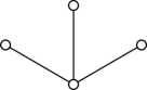
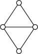
Figure 2.1: Claw and diamond

The claw and the diamond are the two graphs represented Figure 2.1.

Theorem 2.20 (Harary and Holzmann [52])

A graph $G$ is the line-graph of a triangle-free graph if and only if $G$ contains no claw and no diamond.

Proof.

Checking that a line-graph of a triangle-free graph contains no claw and no diamond is a routine matter. Conversely, let $G$ be graph with no claw and no diamond. The theorem of Beineke [3] states that there exists a list $\cal L$ of nine graphs such any graph that does not contain a graph from $\cal L$ is a line-graph. One of the nine graphs is the claw and the eight remaining ones all contain a diamond. So, $G=L(R)$ for some graph $R$. Let $R^{\prime}$ be the graph obtained from $R$ by replacing each connected component of $R$ isomorphic to a triangle by a claw. So, $L(R)=L(R^{\prime})=G$. We claim that $R^{\prime}$ is triangle-free. Else let $T$ be a triangle of $R^{\prime}$. From the construction of $R^{\prime}$, there is a vertex $v\notin T$ in the connected component of $R^{\prime}$ that contains $T$. So we may choose $v$ with a neighbor in $T$. Now the edges of $T$ and one edge from $v$ to $T$ induce a diamond of $G$, a contradiction. ∎

The Harary and Holzmann’s theorem is in a sense a decomposition theorem for graphs with no claw and no diamond. It states that all these graphs are basic. It is likely that no much deeper structural description can be found, because Whitney proved that except for the claw and the triangle (which have the same line-graph), two different graphs have different line-graphs. This yields the following corollary:

Theorem 2.21 (Whitney [108])

If $G$ is a line-graph of a triangle-free graph then there exists a unique graph $R$ such that $G=L(R)$.

So, being able to decompose line-graphs of triangle-free graphs would certainly imply a structural description of all triangle free graphs. Such a description is a well known difficult open question linked to difficult Ramsey Theory as suggested in Chapter 1. More generally, a statement on all line-graphs is likely to be translatable into a statement on all graphs. So, line-graphs behave a bit like sparse graphs of Section 2.3. Strangely, their generality make them basic, and once line-graphs are identified as a substantial subclass of a class, they are likely to form a basic class. This phenomenon occurs in the perhaps two deepest known decomposition theorems: the decomposition of Berge graphs by Chudnovsky, Robertson Seymour and Thomas and the decomposition of claw-free graphs by Chudnovsky and Seymour, see the next section.

2.5 Claw and coclaw

Chudnovsky and Seymour proved a deep structural description of claw-free graphs [19]. The statement is very long and we will not deal with this result in the rest of this work. Here we focus on something much simpler: graphs that are claw-free and whose complements are claw-free. As we will see, these graphs form a very restricted class.

The coclaw is the complement of the claw. The line-graph of $K_{3,3}$ is represented on Figure 2.2. We denote by $A_{6}$ the graph obtained from a triangle by adding for each edge of the triangle, a vertex complete to that edge. The following theorem is due to Pouzet and Si Kaddour but the proof is mine.

Theorem 2.22 (Pouzet and Si Kaddour)

The class ${\rm Forb}\{{\rm claw},$ ${\rm co\-claw}\}$ consists of $A_{6}$, of the induced subgraphs of $L(K_{3,3})$, of graphs whose connected components consist of cycles of length at least 4 and paths, and of the complements of all these graphs.

Proof.

Let $G$ be in the class.

(14) We may assume that $G$ and $\overline{G}$ are connected.

Else, up to symmetry, $G$ is disconnected. If $G$ contains a vertex $v$ of degree at least $3$, then $N(v)$ contains an edge (for otherwise there is a claw), so $G$ contains a triangle. This is a contradiction since by picking a vertex in another component we obtain a coclaw. So all vertices of $G$ are of degree at most 2. It follows that the components of $G$ are cycles (of length at least 4, or there is a coclaw) or paths, an outcome of the theorem. This proves (14).

(15) We may assume that $G$ contains no induced $P_{6}$.

Else $G$ has an induced subgraph $H$ that is either a path on at least 6 vertices or a cycle on at least 7 vertices. Assume $H$ maximal with respect to this property. If $G=H$, an outcome of the theorem is satisfied. Else, by (2.5), we pick a vertex $v$ in $G\setminus H$ with at least one neighbor in $H$. From the maximality of $H$, $v$ has a neighbor $p_{i}$ in the interior of some $P_{6}=p_{1}\!-\!p_{2}\!-\!p_{3}\!-\!p_{4}\!-\!p_{5}\!-\!p_{6}$ of $H$. Up to symmetry we assume that $v$ has a neighbor $p_{i}$ where $i\in\{2,3\}$. So $N(v)\cap\{p_{1},p_{2},p_{3},p_{4}\}$ contains an edge $e$ for otherwise $\{p_{i},p_{i-1},p_{i+1},v\}$ induces a claw. If $e=p_{1}p_{2}$ then $v$ must be adjacent to $p_{4},p_{5},p_{6}$ for otherwise there is a coclaw; so $\{v,p_{1},p_{4},p_{6}\}$ induces a claw. If $e=p_{2}p_{3}$ then $v$ must be adjacent to $p_{5},p_{6}$ for otherwise there is a coclaw, so from the symmetry between $\{p_{1},p_{2}\}$ and $\{p_{5},p_{6}\}$ we may rely on the previous case. If $e=p_{3}p_{4}$ then $v$ must be adjacent to $p_{1},p_{6}$ for otherwise there is a coclaw; so $\{v,p_{1},p_{3},p_{6}\}$ induces a claw. In all cases there is a contradiction. This proves (15).

(16) We may assume that $G$ contains no $A_{6}$ and no $\overline{A_{6}}$.

Else up to a complementation, let $aa^{\prime}$, $bb^{\prime}$, $cc^{\prime}$ be three disjoint edges of $G$ such that the only edges between them are $ab$, $bc$, $ca$. If $V(G)=\{a,a^{\prime},b,b^{\prime},c,c^{\prime}\}$, an outcome of the theorem is satisfied, so let $v$ be a seventh vertex of $G$. We may assume that $av\in E(G)$ (else there is a coclaw). If $a^{\prime}v\in E(G)$ then $vb^{\prime},vc^{\prime}\in E(G)$ (else there is a coclaw) so $\{v,a^{\prime},b^{\prime},c^{\prime}\}$ is a claw. Hence $a^{\prime}v\notin E(G)$. We have $vb\in E(G)$ (or $\{a,a^{\prime},v,b\}$ is a claw) and similarly $vc\in E(G)$. So $\{a^{\prime},v,b,c\}$ is a coclaw. This proves (16).

(17) We may assume that $G$ contains no diamond.

We prefer to think about this in the complement, so suppose for a contradiction that $G$ contains a co-diamond, that is four vertices $a,b,c,d$ that induce only one edge, say $ab$. By (2.5), there is a path $P$ from $\{c,d\}$ to some vertex $w$ that has a neighbor in $\{a,b\}$. We choose such a path $P$ minimal and we assume up to symmetry that the path is from $c$.

If $w$ is adjacent to both $a,b$ then $\{a,b,w,d\}$ induces a coclaw unless $w$ is adjacent to $d$. But in this case, $w$ is adjacent to $c$ from the minimality of $P$, so $\{w,a,c,d\}$ induces a claw. Hence $w$ is adjacent to exactly one of $a,b$, say to $a$. So, $P^{\prime}=c\!-\!P\!-\!w\!-\!a\!-\!b$ is a path and for convenience we rename its vertices $p_{1},\dots,p_{k}$. If $d$ has a neighbor in $P^{\prime}$ then, from the minimality of $P$, this neighbor must be $p_{2}$. So, $\{p_{2},p_{1},p_{3},d\}$ induces a claw. Hence, $d$ has no neighbor in $P^{\prime}$.

By (2.5), there is a path $Q$ from $d$ to some vertex $v$ that has a neighbor in $P^{\prime}$. We choose $Q$ minimal with respect to this property. From the paragraph above, $v\neq d$. Let $p_{i}$ (resp. $p_{j}$) be the neighbor of $v$ in $P^{\prime}$ with minimum (resp. maximum) index. If $i=j=1$ then $d\!-\!Q\!-\!v\!-\!p_{1}\!-\!P\!-\!p_{k}$ is a path on a at least 6 vertices a contradiction to (2.5). So, if $i=j$ then $i\neq 1$ and symmetrically, $i\neq k$, so $\{p_{i-1},p_{i},p_{i+1},v\}$ is a claw. Hence $i\neq j$. If $j>i+1$ then $\{v,v^{\prime},p_{i},p_{j}\}$, where $v^{\prime}$ is the neighbor of $v$ along $Q$, is a claw. So, $j=i+1$. So $vp_{i}p_{j}$ is a triangle. Hence $P^{\prime}=p_{1}\!-\!p_{2}\!-\!p_{3}\!-\!p_{4}$, $Q=d\!-\!v$ and $i=2$, for otherwise there is a coclaw. Hence, $P^{\prime}\cup Q$ form an induced $\overline{A_{6}}$ of $G$, a contradiction to (2.5). This proves (17).

Now $G$ is connected and contains no claw and no diamond. So, by Theorem 2.20, $G$ is the line-graph of some connected triangle-free graph $R$.

If $R$ contains a vertex $v$ of degree at least 4 then all edges of $R$ must be incident to $v$, for else an edge $e$ non-incident to $a$ together with three edges of $R$ incident to $a$ and non-incident to $e$ form a coclaw in $G$. So all vertices of $R$ have degree at most 3. We may assume that $R$ has a vertex $a$ of degree 3 for otherwise $G$ is a path or a cycle. Let $b,b^{\prime},b^{\prime\prime}$ be the neighbors of $a$. Since $a$ has degree 3, all edges of $R$ must be incident to $b,b^{\prime}$ or $b^{\prime\prime}$ for otherwise $G$ contains a coclaw.

If one of $b,b^{\prime},b^{\prime\prime}$, say $b$, is of degree 3, then $N(b)=\{a,a^{\prime},a^{\prime\prime}\}$ and all edges of $R$ are incident to one of $a,a^{\prime},a^{\prime\prime}$ (or there is a coclaw). So $R$ is a subgraph of $K_{3,3}$. So, $G=L(R)$ is an induced subgraph of $L(K_{3,3})$, an outcome of the theorem. Hence we assume that $b,b^{\prime},b^{\prime\prime}$ are of degree at most 2. If $|N(\{b,b^{\prime},b^{\prime\prime}\})\setminus\{a\}|\geq 3$, then $R$ contains the pairwise non-incident edges $bc,b^{\prime}c^{\prime},b^{\prime\prime}c^{\prime\prime}$ say, and the edges $ab,ab^{\prime},ab^{\prime\prime},bc,b^{\prime}c^{\prime},b^{\prime\prime}c^{\prime\prime}$ are vertices of $G$ that induce an $\overline{A_{6}}$, a contradiction to (2.5). So, $|N(\{b,b^{\prime},b^{\prime\prime}\})\setminus\{a\}|\leq 2$ which means again that $R$ is a subgraph of $K_{3,3}$. ∎

An interesting feature of the theorem above is the presence of sporadic graphs: basic graphs are almost all in quite regular classes (here paths and cycles) but there is a finite number of sporadic exceptions (here $A_{6}$ and $L(K_{3,3})$). How sporadic graphs pop up in decomposition theorems is something quite fascinating. In graph theory, these exceptions seem to be member a small club: the five platonic graphs ($K_{4}$, the cube, the octahedron, the dodecahedron and the icosahedron), the Wagner graph, the Petersen graph, the Heawood graph, graphs related to the Fano plane, $K_{3,3}$ and its line-graph, and several more. I wonder who put them here…

Figure 2.2: $L(K_{3,3})$ and its complement

Let me give an entertaining example (from my thesis) of how a sporadic graph appears in a completely unexpected context. On Figure 2.2 is represented $L(K_{3,3})$ with vertices naturally labeled. Next to it is represented its complement with the same labels on the vertices. Note that the two graphs are different: two vertices are adjacent in the first one if and only if they are not in the second. But as one can see, the two graphs are isomorphic, showing that $L(K_{3,3})$ is self-complementary. The entertaining fact is the following: when one sums up the numbers from one row, or one column, or one diagonal of the second square, the result is always 15. So, the nine numbers on the second graphs form what is usually called a magical square, something very famous in mathematical puzzles. This magical square was known by Chinese mathematicians as early as 650 BC (according to Wikipedia), but they certainly ignored that this was related to the biggest self-complementary line-graph…

Examples of sporadic graphs are present in this document: the Wagner graph plays an essential role in the proof of Lemma 1.16, the cube and $K_{4}$ with all edges subdivided are sporadic exceptions in Theorem 3.26, Petersen and Heawood graphs are sporadic in Theorem 4.1, the octahedron is present in Lemmas 4.21 and 4.19.

2.6 Weakly triangulated graphs

A hole or an antihole is said to be long if it contains at least 5 vertices. A graph is weakly triangulated if it contains no long hole and no long antihole. Weakly triangulated graphs were investigated by Chvátal and Hayward in the eighties and the aim of this section is to convince the reader that they can be considered today as one of the most interesting classes of perfect graphs. Because with them, one can understand several important concepts by just reading six pages: Roussel-and-Rubio-like Lemmas, how to deal with antiholes, how uncomfortable decompositions like skew partitions come into the game, why they are uncomfortable, how we can sometimes get rid of them with special vertices (namely even pairs) and thus obtain fast and simple coloring algorithms.

The Roussel and Rubio Lemma [96] is an important technical tool to prove the Strong Perfect Graph Theorem. The team who proved the Strong Perfect Graph Conjecture rediscovered it and called it at some step the “wonderful lemma” because of its many applications. It states that in a sense, any anticonnected set of vertices of a Berge graph behaves like a single vertex (where anticonnected means connected in the complement). How a vertex $v$ “behaves” in a Berge graph? If a path of odd length (at least 3) has both ends adjacent to $v$, then $v$ must have other neighbors in the path for otherwise there is an odd hole. An anticonnected set $T$ of vertices behaves similarly: if a path of odd length (at least 3) has both ends complete to $T$, then at least one interior vertex of the path is also complete to $T$. In fact, there are two exceptions to this statement, so the Roussel and Rubio Lemma is slightly more complicated, and we do not state it here (we do not need it the rest of the document). For more about Roussel and Rubio Lemma, in particular equivalent statements and short proofs, see Chapter 4 of [103].

Here is a lemma which can be seen as a version of the Roussel and Rubio Lemma [96] for weakly triangulated graphs.

Lemma 2.23 (with Maffray [79])

Let $G$ be a weakly triangulated graph. Let $P=x\!-\!\cdots\!-\!y$ be a path of $G$ of length at least 3 and $T\subseteq V(G)$ disjoint from $V(P)$ such that $G[T]$ is anticonnected and the ends of $P$ are $T$-complete. Then $P$ has an interior-vertex which is $T$-complete.

Proof.

Note that no vertex $t\in T$ can be non-adjacent to two consecutive vertices of $P$, for otherwise $V(P)\cup\{t\}$ contains a long hole. Let $z$ be an interior vertex of $P$ adjacent to a maximum number of vertices of $T$. Suppose for a contradiction that there exists a vertex $u\in T\setminus N(z)$. Let $x^{\prime}$ and $y^{\prime}$ be the neighbors of $z$ along $P$, so that $x,x^{\prime},z,y^{\prime},y$ appear in this order along $P$. Then, from the first sentence of this proof, $ux^{\prime},uy^{\prime}\in E(G)$. Up to a relabelling of $x$ and $y$, we assume $x^{\prime}\neq x$. From the choice of $z$, since $ux^{\prime}\in E(G)$ and $uz\notin E(G)$, there exists a vertex $v\in T$ such that $vz\in E(G)$ and $vx^{\prime}\notin E(G)$. Since $G[T]$ is anticonnected, there exists an antipath $Q$ of $G[T]$ from $u$ to $v$, and $u,v$ are chosen subject to the minimality of this antipath. From the first sentence, interior vertices of $Q$ are all adjacent to $x^{\prime}$ or $z$ and from the minimality of $Q$, interior vertices of $Q$ are all adjacent to $x^{\prime}$ and $z$. If $x^{\prime}x\notin E(G)$ then $V(Q)\cup\{x,x^{\prime},z\}$ induces a long antihole. So $x^{\prime}x\in E(G)$. If $zy\notin E(G)$ then $V(Q)\cup\{z,x^{\prime},y\}$ induces a long antihole. So $zy\in E(G)$ and $y=y^{\prime}$. But then, $V(Q)\cup\{x,x^{\prime},z,y\}$ induces a long antihole, a contradiction. ∎

When $T$ is a set of vertices, $C(T)$ denotes the set of these vertices that are complete to $T$.

Lemma 2.24

Let $G$ be a weakly triangulated graph and $T$ a set of vertices such that $G[T]$ is anticonnected and $C(T)$ contains at least two non-adjacent vertices. Suppose that $T$ is inclusion-wise maximal with respect to these properties. Then any path of $G\setminus T$ whose ends are in $C(T)$ has all its vertices in $C(T)$.

Proof.

Let $P$ be a path of $G\setminus T$ whose ends are in $C(T)$. If some vertex of $P$ is not in $C(T)$ then $P$ contains a subpath $P^{\prime}$ of length at least 2 whose ends are in $C(T)$ and whose interior is disjoint from $C(T)$. If $P^{\prime}$ is of length 2, say $P^{\prime}=a\!-\!t\!-\!b$ then $T\cup\{t\}$ is a set which contradicts the maximality of $T$. If $P$ is of length greater than 2, it contradicts Lemma 2.23. ∎

The following theorem is due to Hayward but the proof given here is mine. My proof is not really shorter than Hayward’s, but it shows how Roussel-and-Rubio-like lemmas can be used. A cutset of a graph is a set $S$ of vertices such that $G\setminus S$ is disconnected. A star of a graph is a set of vertices $S$ that contain a vertex $c$ such that $S\subseteq N[c]$. A star cutset is a star that is a cutset.

Theorem 2.25 (Hayward [54])

Let $G$ be a weakly triangulated graph. Then either:

• $G$ is a clique;

• $G$ is the complement of a perfect matching;

• $G$ admits a star cutset.

Proof.

If $G$ is a disjoint union of cliques (in particular when $|V(G)|\leq 2$) then the theorem holds trivially. So by Theorem 2.1, we may assume that $G$ contains a $P_{3}$. Hence, there exists a set $T$ of vertices such that $G[T]$ is anticonnected and $C(T)$ contains at least two non-adjacent vertices because the middle of a $P_{3}$ forms such a set. Let us assume $T$ maximal like in Lemma 2.24. Since $C(T)$ is not a clique, by induction we have two cases to consider:

Case 1: the graph induced by $C(T)$ has a star cutset $S$. From Lemma 2.24, $T\cup S$ is a star cutset of $G$.

Case 2: the graph induced by $C(T)$ is the complement of a perfect matching.

Suppose first that $V(G)=T\cup C(T)$. Then by induction, either $T=\{t\}$, of $T$ induces the complement of a perfect matching or $T$ has a star cutset $S$. But in the first case, $\{t\}\cup C(T)\setminus\{a,b\}$ where $a,b$ are non-adjacent in $C(T)$, is a star cutset of $G$. In the second case, $G$ itself is the complement of a perfect matching. In the third case, $S\cup C(T)$ is a star cutset of $G$.

So, we may assume that there exists a vertex $x\in V(G)\setminus(T\cup C(T))$. We choose $x$ with a neighbor $y$ in $C(T)$, this is possible otherwise $T$ together with any vertex of $C(T)$ forms a star cutset of $G$.

Recall that $C(T)$ is the complement of a perfect matching. So, let $y^{\prime}$ be the non-neighbor of $y$ in $C(T)$. Note that $xy^{\prime}\notin E(G)$ for otherwise $T\cup\{x\}$ would contradict the maximality of $T$. We claim that $S=T\cup C(T)\setminus\{y^{\prime}\}$ is a star cutset of $G$ separating $x$ from $y^{\prime}$. First it is a star centered $y$. And it is a cutset because if there a path in $G\setminus S$ from $x$ to $y^{\prime}$, then by appending $y$ to that path we see that $G\setminus T$ contains a path from $y$ to $y^{\prime}$ that is not included in $C(T)$, a contradiction to Lemma 2.24. ∎

From the theorem above and the following one, weakly triangulated graphs are perfect. To see this, consider a non-perfect weakly triangulated graph, and vertex-inclusionwise minimal with respect to this property. So, it is a minimally imperfect graph (that is a non-perfect graph whose all induced subgraphs are perfect). Since cliques and complement of perfect matchings are perfect, it must have a a star cutset by Theorem 2.25. So, it contradicts the following (proof is omitted here).

Theorem 2.26 (Chvátal [22])

A minimally imperfect graph has no star cutset.

Theorem 2.25 has a disease: it uses the star cutset which is the simplest example of what Kristina Vušković calls strong cutsets: kinds of cutsets that do not give much structure. To see this, note that a star cutset can be very big. For instance, it can be the whole vertex-set except two vertices. And since in the cutset itself, edges are quite unconstrained, knowing that the graph has a star cutset tells little about its structure. Another famous example of a strong cutset that we will meet and define is the skew partition, see Section 5.1.

Strong cutsets do not give structure theorems. To see this, try to see how to build a graph by gluing two smaller graphs along a star. This is likely to be unsatisfactory. Because finding the same star in two graphs is algorithmically quite difficult. It supposes that one can check whether two stars are isomorphic, a problem as difficult as the well known open isomorphism problem. Well, there is no formal notion of what is a structure theorem, so there can be endless discussions on this. But one can feel that gluing along star cutsets is less automatic than gluing along 2-cutsets like in Section 2.3.

Strong cutset are difficult to use in polynomial time algorithms. Because to build blocks of decomposition with them, in the unlucky case where the cutset is almost as big as the graph, one has to keep almost all the graph in both blocks of decomposition. So recursive algorithms using strong cutset typically take exponential time. A technically involved method invented by Conforti and Rao [29, 30], the so-called cleaning, allows to devise fast recognition algorithms for classes decomposed by strong cutsets. But for combinatorial optimization problems, it seems that no one knows how to use strong cutsets. Yet, when a class of graphs is complex enough so that strong cutsets seem unavoidable, there is still a hope. Indeed, several theorems replace cutsets with the existence of a vertex or a pair of vertices with very special properties. The oldest example is the following, to be compared with Theorem 2.4. A simplicial vertex is a vertex whose neighborhood is a clique.

Theorem 2.27 (Dirac, [39])

Any chordal graph contains a simplicial vertex.

For perfect graphs, the good notion of special vertices seems to be the even pair. An even pair of vertices is a pair of vertices such that all paths linking them are of even length. By the following theorem, even pairs are a good tool for proving perfectness.

Theorem 2.28 (Meyniel [86])

A minimally imperfect graph has no even pair.

Contracting an even pair $a,b$ means replacing $a,b$ by a single vertex complete to $N(a)\cup N(b)$. By the following theorem, even pairs are also a good tool for graph coloring.

Theorem 2.29 (Fonlupt and Uhry [42])

Contracting an even pair of a graph preserves its chromatic number and the size of a largest clique.

The following theorem was first proved by Hayward, Hoàng and Maffray but the proof given here was obtained jointly with Maffray in [79]. A 2-pair $a,b$ is a special kind of even pair: all paths from $a$ to $b$ are of length 2.

Theorem 2.30 (Hayward, Hoàng and Maffray [53])

A weakly triangulated graph either is a clique or admits a 2-pair.

Proof.

If $G$ is a disjoint union of cliques (in particular when $|V(G)|\leq 2$) then the theorem holds trivially. So we may assume that $G$ contains a $P_{3}$. So, there exists a set $T$ like in Lemma 2.24 (start with the middle of a $P_{3}$ to build $T$). Since $C(T)$ is not a clique, by induction we know that $C(T)$ admits a 2-pair of $G[C(T)]$. From Lemma 2.24 it is a 2-pair of $G$. ∎

The technique above to find an even pair can be backtracked to the seminal paper of Henri Meyniel [86], see Exercise 2.32 below. Using ideas of Cláudia Linhares Sales and Maffray [70], this technique can be extended to Artemis graphs [79], which are a generalization of several classes of perfect graphs known to have even pairs (weakly triangulated graphs, Meyniel graphs and perfectly orderable graphs etc; we shall not define all the classes, a reader who want to visit the zoo can read Chapter 3 of [103]). The technicalities in [79] together with new kinds of special vertices and complicated variations on the Roussel and Rubio Lemma are used by Chudnovsky and Seymour [18] to shorten significantly the proof of the Strong Perfect Graph Theorem.

From the Theorem 2.30, it is easy to deduce a polynomial time algorithm for coloring weakly triangulated graphs (by contracting 2-pairs as long as there are some). Hayward, Spinrad and Sritharan [55] could speed this algorithm up to $O(n^{3})$. Since the contraction of a 2-pair preserves both $\chi$ and $\omega$, the algorithm will transform any weakly triangulated graph $G$ into a clique $K$ of size $\omega(G)=\omega(K)=\chi(K)=\chi(G)$, thus proving the perfectness of $G$ (because all this can be done for all induced subgraphs of $G$). So, Theorem 2.30 gives in fact a much shorter proof of the perfectness of weakly triangulated graphs.

Berge graphs behave in a way like weakly triangulated graphs. The Roussel and Rubio Lemma is an important tool to prove their perfectness, a strong cutset is needed to decompose them (the so-called balanced skew partition), but by using even pairs, a shorter proof of perfectness can be found (this was done by Chudnovsky and Seymour [18]). A big difference of course is that for general Berge graphs all the proofs are much longer and highly technical. And up to now, no fast combinatorial coloring algorithm for Berge graphs is known. But it might be that even pairs become an ingredient of such an algorithm. A collection of theorems and conjectures supports this idea, but a heavy machinery is needed just to state all them, so we postpone this to Section 5.7.

Another important open question about Berge graphs is the existence of a structure theorem for them. The following is seemingly easier but remains open.

Question 2.31

Find a structure theorem for weakly triangulated graphs.

In fact, I would not be surprised that no structure theorem exists for Berge graphs. It would be great to have a tool like NP-completeness to get people convinced of such negative statements, or better to prove them. The non-existence of a polynomial time recognition algorithm could be an argument, but it does not work for Berge graphs that can be recognized in $O(n^{9})$ as mentioned in the introduction.

Another well known class was seminal to many ideas in the theory of perfect graphs: Meyniel graphs. A graph is Meyniel if all its odd cycles of length at least 5 admit at least two chords. Meyniel graphs were proved to be perfect very early by Meyniel [85], and were the first class after chordal and $P_{4}$-free graphs for which a decomposition theorem could be proved (by Burlet and Fonlupt [9]). With respect to even pairs, Meyniel graphs have behavior similar to weakly triangulated graphs. We leave this as an exercise.

Exercise 2.32

Give a version of the Roussel and Rubio lemma for Meyniel graphs. Deduce that a Meyniel graph either is a clique or has an even pair. For a solution, see [86].

Chapter 3 Detecting induced subgraphs

Recognizing a class of graph means giving an algorithm that decides whether an input graph is in the class. This can be of practical interest (does a network satisfy this or that condition, maybe an application of what follows can be cooked …). But for us, recognizing classes of graphs is mainly of a theoretical interest. It is a tool to classify classes: those that are NP-complete to recognize are unlikely to have a very precise decomposition theorem. This criterion is not to be taken too religiously. Some classes are trivial to recognize in polynomial time while their structure is unknown or highly non-trivial, for instance triangle-free graphs and claw-free graphs. Some classes have a decomposition theorem not precise enough to give a polynomial-time recognition algorithm (for instance odd hole-free graphs, see Theorem 5.1). But it is nice to have a general criterion about what class is “understood”. Together with $\chi$-boundness, the existence of a fast recognition algorithm is the only criterion applying to any class that we are aware of.

The classes we are working on are defined by forbidding a list of induced subgraphs. So recognizing one of them is equivalent to being able to decide whether a given graph contains one graph from the list. In its full generality, this problem is known to be difficult from the very beginning of Complexity Theory, even for lists of size one.

Theorem 3.1 (Cook [31])

The following problem is NP-complete.

Instance

Two graphs $G$ and $H$.

Question

Does $G$ contain an induced subgraph isomorphic to $H$?

On the other hand, the following is trivial by a brute force algorithm.

Theorem 3.2

Let $H$ be a graph. The following problem can be solved in time $O(n^{|V(H)|})$.

Instance

A graph $G$.

Question

Does $G$ contain an induced subgraph isomorphic to $H$?

The brute-force method above is the source of many algorithms with strange running times (the worst I will mention runs in time $O(n^{18})$, see the end of Section 3.2). These complexities are bad, but not as bad as one might expect. Suppose for instance that an algorithm uses as a subroutine an enumeration of all subsets on 18 vertices of an input graph. So, the complexity is very bad. It is sometimes said that $O(n^{18})$-algorithms are useless in practice and that an algorithm of complexity $O(2^{n})$ is better for any reasonable $n$ (because $2^{30}<30^{18}$ say). This can be true for some particular algorithms, but is completely false for some others. To see this, consider the brute-force algorithm to enumerate all subsets of size 18 from a set on $n$ elements (complexity $O(n^{18})$). Is it worse than enumerating all the subsets (complexity $O(2^{n})$)? Certainly not: there are many more subsets than subsets on 18 elements! Because the constant hidden in the $O$ matters, and it is a mistake to think that this constant can only bring trouble. In some situations, the constant is much smaller than 1, and enumerating subsets on $k$ elements is an example (because ${n\choose k}<n^{k}$). Anyway, comparing blindly big-$O$’s for practical reasons is not very wise. For practical applications, only the actual running time matters and complexity theory just gives a possibly misleading indication.

To produce something between trivial polynomiality and NP-completeness, we need to consider the problem of detecting an induced subgraph from a fixed infinite list. But this is far much too general. To see this, consider the following question that should not be too difficult. It should suffice to encode any Turing machine as a graph and to define $\cal L$ as something related to the halting problem.

Question 3.3

Define a list $\cal L$ of graphs such that deciding whether a graph contains an element of $\cal L$ as an induced subgraph is an undecidable problem.

So, to produce something interesting, we need to give some structure to the list of forbidden induced subgraphs. In many interesting problems, the list of forbidden induced subgraphs is obtained by subdividing prescribed edges of a prescribed graph. This lead Lévêque, Maffray and myself [68] to the following definitions.

A subdivisible graph (s-graph for short) is a triple $B=(V,D,F)$ such that $(V,D\cup F)$ is a graph and $D\cap F=\emptyset$. The edges in $D$ are said to be real edges of $B$ while the edges in $F$ are said to be subdivisible edges of $B$. A realisation of $B$ is a graph obtained from $B$ by subdividing edges of $F$ into paths of arbitrary length (at least one). The problem $\Pi_{B}$ is the decision problem whose input is a graph $G$ and whose question is ”Does $G$ contain a realisation of $B$ as an induced subgraph?”. On figures, we depict real edges of an s-graph with straight lines, and subdivisible edges with dashed lines.

$B_{1}$		$B_{2}$		$B_{3}$

Figure 3.1: Pyramids, prisms and thetas

We shall study several instances of $\Pi_{B}$ and survey the efficient methods to tackle them. Some $\Pi_{B}$’s are NP-complete, some are polynomial, and many remain open. As an appetizer, let us give now several examples. A pyramid (resp. prism, theta) is any realisation of the s-graph $B_{1}$ (resp. $B_{2}$, $B_{3}$) represented on Figure 3.1. Chudnovsky and Seymour [13] gave an $O(n^{9})$-time algorithm for $\Pi_{B_{1}}$ (or equivalently, for detecting a pyramid). As far as we know, that is the first example of a solution to a $\Pi_{B}$ whose complexity is non-trivial to settle. The method used is what we call shortest path detector, see Section 3.2. In contrast, we proved jointly with Maffray [78] that $\Pi_{B_{2}}$ (or detecting a prism) is NP-complete. The method relies on a construction due to Bienstock that has many applications, see Section 3.1. Chudnovsky and Seymour [20] gave an $O(n^{11})$-time algorithm for $P_{B_{3}}$ (or detecting a theta). Their algorithm relies on the solution of a problem called “three-in-a-tree”, that has many applications, see Section 3.3. In Section 3.4 we present several variations on three-in-a-tree.

Note that pyramids, prisms and thetas are sometimes called respectively 3PC($\Delta$, $\cdot$), 3PC($\Delta$, $\Delta$), 3PC($\cdot$, $\cdot$) where “3PC” means three paths configurations. This is sometimes a very convenient notation.

Often, forbidding 3PC’s yields interesting classes. Note for instance that Berge graphs contain no pyramid and even-hole-free graphs contain no prisms and no thetas.

From the examples above one can feel that strangely close s-graphs lead to drastically different complexities (as far as P$\neq$NP). Before going into the details, let us give a last example may be more striking than pyramid/prism/theta : $\Pi_{B_{4}},\Pi_{B_{6}}$ are polynomial and $\Pi_{B_{5}},\Pi_{B_{7}}$ are NP-complete, where $B_{4},\dots,B_{7}$ are the s-graphs represented on Figure 3.2, see Theorem 3.14.

$B_{4}$		$B_{5}$		$B_{6}$		$B_{7}$

Figure 3.2: Some s-graphs with pending edges

3.1 A tool for NP-completeness: Bienstock’s Construction

In 1991, Dan Bienstock published a paper [6] with an NP-completeness proof that can be applied in many situations (with slight variations). I am grateful to Bienstock because out of the ten accepted/published papers I have today, six contain results relying on Bienstock’s construction, and three more mention NP-completeness results relying on it.

Let $\cal S$ be a set of graphs and $d$ an integer. Let $\Gamma_{\cal S}^{d}$ be the problem whose instance is $(G,x,y)$ where $G$ is a graph such that $\Delta(G)\leq d$, with no induced subgraph in $\cal S$ and $x,y\in V(G)$ are two non-adjacent vertices of degree $2$. The question is “Does $G$ contain a hole passing through $x,y$?”. For simplicity, we write $\Gamma_{\cal S}$ instead of $\Gamma_{\cal S}^{+\infty}$ (so, the graph in the instance of $\Gamma_{\cal S}$ has unbounded degree). Also we write $\Gamma^{d}$ instead of $\Gamma^{d}_{\emptyset}$ (so the graph in the instance of $\Gamma^{d}$ has no restriction on its induced subgraphs). Bienstock [6] proved that $\Gamma=\Gamma_{\emptyset}$ is NP-complete. Here we give the simplest proof that we are aware of using Bienstock’s construction. This is from a paper with Maffray [78] and is slightly simpler than the original construction.

Theorem 3.4

Problem $\Gamma_{\{K_{3}\}}$ is NP-complete

Proof.

Let us give a polynomial reduction from the problem $3$-Satisfiability of Boolean functions to problem $\Gamma_{\{K_{3}\}}$. Recall that a Boolean function with $n$ variables is a mapping $f$ from $\{0,1\}^{n}$ to $\{0,1\}$. A Boolean vector $\xi\in\{0,1\}^{n}$ is a truth assignment for $f$ if $f(\xi)=1$. For any Boolean variable $x$ on $\{0,1\}$, we write $\overline{x}:=1-x$, and each of $x,\overline{x}$ is called a literal. An instance of $3$-Satisfiability is a Boolean function $f$ given as a product of clauses, each clause being the Boolean sum $\vee$ of three literals; the question is whether $f$ admits a truth assignment.

Let $f$ be an instance of $3$-Satisfiability, consisting of $m$ clauses $C_{1},\ldots,C_{m}$ on $n$ variables $x_{1},\ldots,x_{n}$. Let us build a graph $G_{f}$ with two specialized vertices $a,b$, such that there will be a hole containing both $a,b$ in $G$ if and only if there exists a truth assignment for $f$.

For each variable $x_{i}$ ($i=1,\ldots,n$), make a graph $G(x_{i})$ with eight vertices $a_{i},b_{i},t_{i},f_{i},a^{\prime}_{i},b^{\prime}_{i},t^{\prime}_{i},f^{\prime}_{i},$ and ten edges $a_{i}t_{i},a_{i}f_{i},b_{i}t_{i},b_{i}f_{i}$ (so that $\{a_{i},b_{i},t_{i},f_{i}\}$ induces a hole), $a^{\prime}_{i}t^{\prime}_{i},a^{\prime}_{i}f^{\prime}_{i},b^{\prime}_{i}t^{\prime}_{i},b^{\prime}_{i}f^{\prime}_{i}$ (so that $\{a^{\prime}_{i},b^{\prime}_{i},t^{\prime}_{i},f^{\prime}_{i}\}$ induces a hole) and $t_{i}f^{\prime}_{i},t^{\prime}_{i}f_{i}$. See Figure 3.3.

Figure 3.3: Graph $G(x_{i})$

Figure 3.4: Graph $G(C_{j})$

Figure 3.5: The two edges added to $G_{f}$ in the case $u_{j}^{p}=x_{i}$

Figure 3.6: Graph $G_{f}$

For each clause $C_{j}$ ($j=1,\ldots,m$), with $C_{j}=u_{j}^{1}\vee u_{j}^{2}\vee u_{j}^{3}$, where each $u_{j}^{p}$ ($p=1,2,3$) is a literal from $\{x_{1},\ldots,x_{n},\overline{x}_{1},\ldots,\overline{x}_{n}\}$, make a graph $G(C_{j})$ with five vertices $c_{j},d_{j},v_{j}^{1},v_{j}^{2},v_{j}^{3}$ and six edges so that each of $c_{j},d_{j}$ is adjacent to each of $v_{j}^{1},v_{j}^{2},v_{j}^{3}$. See Figure 3.4. For $p=1,2,3$, if $u_{j}^{p}=x_{i}$ then add two edges $u_{j}^{p}f_{i},u_{j}^{p}f^{\prime}_{i}$, while if $u_{j}^{p}=\overline{x}_{i}$ then add two edges $u_{j}^{p}t_{i},u_{j}^{p}t^{\prime}_{i}$. See Figure 3.5.

The graph $G_{f}$ is obtained from the disjoint union of the $G(x_{i})$’s and the $G(C_{j})$’s as follows. For $i=1,\ldots,n-1$, add edges $b_{i}a_{i+1}$ and $b^{\prime}_{i}a^{\prime}_{i+1}$. Add an edge $b^{\prime}_{n}c_{1}$. For $j=1,\ldots,m-1$, add an edge $d_{j}c_{j+1}$. Introduce the two specialized vertices $a,b$ and add edges $aa_{1},aa^{\prime}_{1}$ and $bd_{m},bb_{n}$. See Figure 3.6. Clearly the size of $G_{f}$ is polynomial (actually linear) in the size $n+m$ of $f$. Moreover, it is easy to see that $G_{f}$ contains no triangle, and that $a,b$ are non-adjacent and both have degree $2$.

Suppose that $f$ admits a truth assignment $\xi\in\{0,1\}^{n}$. We build a hole in $G$ by selecting vertices as follows. Select $a,b$. For $i=1,\ldots,n$, select $a_{i},b_{i},a^{\prime}_{i},b^{\prime}_{i}$; moreover, if $\xi_{i}=1$ select $t_{i},t^{\prime}_{i}$, while if $\xi_{i}=0$ select $f_{i},f^{\prime}_{i}$. For $j=1,\ldots,m$, since $\xi$ is a truth assignment for $f$, at least one of the three literals of $C_{j}$ is equal to $1$, say $u_{j}^{p}=1$ for some $p\in\{1,2,3\}$. Then select $c_{j},d_{j}$ and $v_{j}^{p}$. Now it is a routine matter to check that the selected vertices induce a cycle $Z$ that contains $a,b$, and that $Z$ is chordless, so it is a hole. The main point is that there is no chord in $Z$ between some subgraph $G(C_{j})$ and some subgraph $G(x_{i})$, for that would be either an edge $t_{i}v_{j}^{p}$ (or $t^{\prime}_{i}v_{j}^{p}$) with $u_{j}^{p}=x_{i}$ and $\xi_{i}=1$, or, symmetrically, an edge $f_{i}v_{j}^{p}$ (or $f^{\prime}_{i}v_{j}^{p}$) with $u_{j}^{p}=\overline{x}_{i}$ and $\xi_{i}=0$, in either case a contradiction to the way the vertices of $Z$ were selected.

Conversely, suppose that $G_{f}$ admits a hole $Z$ that contains $a,b$. Clearly $Z$ contains $a_{1},a^{\prime}_{1}$ since these are the only neighbours of $a$ in $G_{f}$.

(18) For $i=1,\ldots,n$, $Z$ contains exactly six vertices of $G_{i}$: four of them are $a_{i},a^{\prime}_{i},b_{i},b^{\prime}_{i}$, and the other two are either $t_{i},t^{\prime}_{i}$ or $f_{i},f^{\prime}_{i}$.

First we prove the claim for $i=1$. Since $a,a_{1}$ are in $Z$ and $a_{1}$ has only three neighbours $a,t_{1},f_{1}$, exactly one of $t_{1},f_{1}$ is in $Z$. Likewise exactly one of $t^{\prime}_{1},f^{\prime}_{1}$ is in $Z$. If $t_{1},f^{\prime}_{1}$ are in $Z$ then the vertices $a,a_{1},a^{\prime}_{1},t_{1},f^{\prime}_{1}$ are all in $Z$ and they induce a hole that does not contain $b$, a contradiction. Likewise we do not have both $t^{\prime}_{1},f_{1}$ in $Z$. Therefore, up to symmetry we may assume that $t_{1},t^{\prime}_{1}$ are in $Z$ and $f_{1},f^{\prime}_{1}$ are not. If a vertex $u_{j}^{p}$ of some $G(C_{j})$ ($1\leq j\leq m$, $1\leq p\leq 3$) is in $Z$ and is adjacent to $t_{1}$ then, since this $u_{j}^{p}$ is also adjacent to $t^{\prime}_{1}$, we see that the vertices $a,a_{1},a^{\prime}_{1},t_{1},t^{\prime}_{1},u_{j}^{p}$ are all in $Z$ and induce a hole that does not contain $b$, a contradiction. Thus the neighbour of $t_{1}$ in $Z\setminus a_{1}$ is not in any $G(C_{j})$ ($1\leq j\leq m$), so that neighbour is $b_{1}$. Likewise $b^{\prime}_{1}$ is in $Z$. So the claim holds for $i=1$. Since $b_{1}$ is in $Z$ and exactly one of $t_{1},f_{1}$ is in $Z$, and $b_{1}$ has degree $3$ in $G_{f}$, we obtain that $a_{2}$ is in $Z$, and similarly $b_{2}$ is in $Z$. Now the proof of the claim for $i=2$ is essentially the same as for $i=1$, and by induction the claim holds up to $i=n$. This proves (18).

(19) For $j=1,\ldots,m$, $Z$ contains $c_{j},d_{j}$ and exactly one of $v_{j}^{1},v_{j}^{2},v_{j}^{3}$.

First we prove this claim for $j=1$. By Claim 3.1, $b^{\prime}_{n}$ is in $Z$ and exactly one of $t^{\prime}_{n},f^{\prime}_{n}$ is in $Z$, so (since $b^{\prime}_{n}$ has degree $3$ in $G_{f}$) $c_{1}$ is in $Z$. Consequently exactly one of $u_{1}^{1},u_{1}^{2},u_{1}^{3}$ is in $Z$, say $u_{1}^{1}$. The neighbour of $u_{1}^{1}$ in $Z\setminus c_{1}$ cannot be a vertex of some $G(x_{i})$ ($1\leq i\leq n$), for that would be either $t_{i}$ (or $f_{i}$) and thus, by Claim 3.1, $t^{\prime}_{i}$ (or $f^{\prime}_{i}$) would be a third neighbour of $u_{1}^{1}$ in $Z$, a contradiction. Thus the other neighbour of $u_{1}^{1}$ in $Z$ is $d_{1}$, and the claim holds for $j=1$. Since $d_{1}$ has degree $4$ in $G_{f}$ and exactly one of $v_{1}^{1},v_{1}^{2},v_{1}^{3}$ is in $Z$, it follows that its fourth neighbour $c_{2}$ is in $Z$. Now the proof of the claim for $j=2$ is the same as for $j=1$, and by induction the claim holds up to $j=m$. This proves (19).

We can now make a Boolean vector $\xi$ as follows. For $i=1,\ldots,n$, if $Z$ contains $t_{i},t^{\prime}_{i}$ set $\xi_{i}=1$; if $Z$ contains $f_{i},f^{\prime}_{i}$ set $\xi_{i}=0$. By (3.1) this is consistent. Consider any clause $C_{j}$ ($1\leq j\leq m$). By (3.1) and up to symmetry we may assume that $v_{j}^{1}$ is in $Z$. If $u_{j}^{1}=x_{i}$ for some $i\in\{1,..,n\}$, then the construction of $G_{f}$ implies that $f_{i},f^{\prime}_{i}$ are not in $Z$, so $t_{i},t^{\prime}_{i}$ are in $Z$, so $\xi_{i}=1$, so clause $C_{j}$ is satisfied by $x_{i}$. If $u_{j}^{1}=\overline{x}_{i}$ for some $i\in\{1,..,n\}$, then the construction of $G_{f}$ implies that $t_{i},t^{\prime}_{i}$ are not in $Z$, so $f_{i},f^{\prime}_{i}$ are in $Z$, so $\xi_{i}=0$, so clause $C_{j}$ is satisfied by $\overline{x}_{i}$. Thus $\xi$ is a truth assignment for $f$. This completes the proof of the theorem. ∎

Now we can see how to use the Theorem above to prove the NP-completeness of a detection problem.

Theorem 3.5 (with Maffray [78])

Problem $\Pi_{B_{2}}$ (deciding whether a graph contains a prism) is NP-complete.

Proof.

Starting from from an instance ($G$, a, b) of $\Gamma_{K_{3}}$, build a graph $G^{\prime}$ as follows (see Figure 3.7): replace vertex $a$ by five vertices $a_{1},a_{2},a_{3},a_{4},a_{5}$ with five edges $a_{1}a_{2}$, $a_{1}a_{3}$, $a_{2}a_{3}$, $a_{2}a_{4}$, $a_{3}a_{5}$, and put edges $a_{4}a^{\prime}$ and $a_{5}a^{\prime\prime}$. Do the same with $b$, with five vertices named $b_{1},\ldots,b_{5}$ instead of $a_{1},\ldots,a_{5}$ and with the analogous edges. Add an edge $a_{1}b_{1}$. Since $G$ has no triangle, $G^{\prime}$ has exactly two triangles $\{a_{1},a_{2},a_{3}\}$ and $\{b_{1},b_{2},b_{3}\}$. Moreover we see that $G^{\prime}$ contains a prism if and only if $G$ contains a hole that contains $a$ and $b$. So every instance of $\Gamma_{\{K_{3}\}}$ can be reduced polynomially to an instance of $\Pi_{B_{2}}$, which proves that $\Pi_{B_{2}}$ is NP-complete. ∎

Figure 3.7: Detecting a prism: $G$ and $G^{\prime}$

Exercise 3.6

Deciding whether a graph contains the line-graph of a subdivision of $K_{4}$ is NP-complete.

Adapting the construction of Bienstock, the following can be proved (it is not so easy to eliminate simultaneously triangles and square, the proof is very tedious so we omit it). We denote by $I_{l}$ ($l\geq 1$) the tree on $l+5$ vertices obtained by taking a path of length $l$ with ends $a,b$, and adding four vertices, two of them adjacent to $a$, the other two to $b$; see Figure 3.8.

Figure 3.8: $I_{1}$

Theorem 3.7 (with Lévêque and Maffray [68])

Let $k\geq 5$ be an integer. Then $\Gamma_{\{C_{3},\dots,C_{k},K_{1,6}\}}$ and $\Gamma_{\{I_{1},\dots,I_{k},C_{5},\dots,C_{k},K_{1,4}\}}$ are NP-complete.

The theorem above will be proved in a sense best possible in Section 3.3 where a dichotomy criterion will be given for the problems $\Gamma_{\{H\}}$ where $H$ is a connected graph, see Theorem 3.15. It has several easy corollaries as the NP-completeness of $\Pi_{B_{5}},\Pi_{B_{7}}$ mentioned above (see Theorem 3.14 below for a proof). Also, it can be used to prove the NP-completeness of the detections of structures analogous to pyramids, prisms and theta but with four paths instead of three (this NP-completeness was in fact obtained jointly with Maffray and Vušković without Theorem 3.7 in [80]). In Section 4.1, an $O(nm)$ algorithm will be given to detect cycles with a unique chord. The Theorem above will then be used to prove the NP-completeness of quite similar detection problems.

The following was proved by David Lin during his Master Thesis, a very nice and surprising result. Since publishing NP-completeness results alone is no more fashionable, we invited Lin in our paper [68]. The Bienstock-like construction that Lin uses is so modified that we can say that Lin found a new construction.

Theorem 3.8 (Lin [68])

$\Gamma^{3}$ is NP-complete.

From Theorem 3.8 it is easy to see that detecting whether a graph contains a subdivision of $K_{5}$ is NP-complete, see [68]. This result is of interest because a major breakthrough of Robertson and Seymour in their Graph Minor Project is that detecting a subdivision of any graph as a possibly non-induced subgraph is a polynomial problem. So, the “induced” constraint really matters and causes trouble.

3.2 A tool for polynomiality (1): shortest path detectors

The shortest path detector is a method designed by Chudnovsky and Seymour [13] to decide whether a graph contains a pyramid. The motivation for detecting pyramids is that every pyramid contains an odd holes. So, when trying to recognize Berge graphs, it is interesting to first look for pyramids.

Theorem 3.9 (Chudnovsky and Seymour [13])

There exists an $O(n^{9})$ algorithm for Problem $\Pi_{B_{1}}$ (deciding whether a graph contains a pyramid).

To explain the method, we give here an algorithm that detects prisms in graphs with no pyramids (recall that in general graphs, the problem is NP-complete). This algorithm is very simple but is not published because a faster one exists, see [78]. A shortest path detector always relies on a Lemma stating in the smallest substructure of the kind that we are looking for, a path linking two particular vertices of the substructure can be replaced by any shortest path.

Lemma 3.10

Let $G$ be a graph with no pyramid. Let $K$ be a smallest prism in $G$. Suppose that $K$ is a prism, formed by paths $P_{1},P_{2},P_{3}$, with triangles $\{a_{1},a_{2},a_{3}\}$ and $\{b_{1},b_{2},b_{3}\}$, so that, for $i=1,2,3$, path $P_{i}$ is from $a_{i}$ to $b_{i}$. Then:

If $R_{i}$ is any shortest path from $a_{i}$ to $b_{i}$ whose interior vertices are not adjacent to $a_{i+1}$, $a_{i+2}$, $b_{i+1}$ or $b_{i+2}$, then $R_{i},P_{i+1},P_{i+2}$ form a prism on $|V(K)|$ vertices in $G$, with triangles $\{a_{1},a_{2},a_{3}\}$ and $\{b_{1},b_{2},b_{3}\}$ (the addition of subscripts is taken modulo 3).

Proof.

Suppose that the lemma fails for say $i=1$. So, some interior vertex of $R$ has neighbors in the interior of $P_{2}$ or $P_{3}$. Let $x$ be such a vertex, closest to $a_{1}$ along $R$. Let $a^{\prime}_{2}$ (resp. $a^{\prime}_{3}$) be the neighbor of $a_{2}$ (resp. $a_{3}$) along $P_{2}$ (resp. $P_{3}$). Let $Q=a^{\prime}_{2}\!-\!P_{2}\!-\!b_{2}\!-\!b_{3}\!-\!P_{3}\!-\!a^{\prime}_{3}$. Let $y$ (resp. $z$) be the neighbor of $x$ closest to $a^{\prime}_{2}$ (resp. $a^{\prime}_{3}$) along $Q$.

If $y=z$ then $y\!-\!x\!-\!R\!-\!a_{1}$, $y\!-\!Q\!-\!a^{\prime}_{2}\!-\!a_{2}$ and $y\!-\!Q\!-\!a^{\prime}_{3}\!-\!a_{3}$ form a pyramid, a contradiction. If $y\neq z$ and $yz\notin E(G)$ then $x\!-\!R\!-\!a_{1}$, $x\!-\!y\!-\!Q\!-\!a^{\prime}_{2}\!-\!a_{2}$ and $x\!-\!z\!-\!Q\!-\!a^{\prime}_{3}\!-\!a_{3}$ form a pyramid, a contradiction. If $yz\in E(G)$ then $x\!-\!R\!-\!a_{1}$, $y\!-\!Q\!-\!a^{\prime}_{2}\!-\!a_{2}$ and $z\!-\!Q\!-\!a^{\prime}_{3}\!-\!a_{3}$ form a prism on less vertices than $K$, a contradiction. ∎

Now detecting a prism in a graph with no pyramid can be performed as follows. For all 6-tuples $(a_{1},a_{2},a_{3},b_{1},b_{2},b_{3})$ compute three shortest paths $R_{i}$ in $G\setminus((N[a_{i+1}]\cup N[a_{i+2}]\cup N[b_{i+1}]\cup N[b_{i+2}])\setminus\{a_{i},b_{i}\})$ from $a_{i}$ to $b_{i}$. Check whether $R_{1},R_{2},R_{3}$ form a prism, and if so output it. If no triple of paths forms a prism, output that the graph contains no prism. If the algorithm outputs a prism, this is obviously a correct answer: the graph contains a prism. Suppose conversely that the graph contains a prism. Then it contains a smallest prism with triangles $\{a_{1},a_{2},a_{3}\}$ and $\{b_{1},b_{2},b_{3}\}$. At some step, the algorithm will check this 6-tuple (unless a prism is discovered before, but then the correctness is proved anyway). By three applications of Lemma 3.10, we see that the three paths $R_{1},R_{2},R_{3}$ form a prism that is output. All this take time $O(n^{8})$.

The method is very beautiful and simple; detecting pyramids in $O(n^{9})$ is more involved. With several tricks, the detection of prisms in graphs with no pyramids can be performed in $O(n^{5})$, see [78]. Shortest path detectors solve several other problems for graphs with no odd holes, see [78], such as the detection of line-graphs of bipartite subdivisions of $K_{4}$ in $O(n^{18})$, even prisms in $O(n^{9})$ and odd prisms in $O(n^{18})$ (where a prism is even (resp. odd) when the three path forming it are of even (resp. even) length). These problems are all of interest because these three substructures are used in the proof of the Strong Perfect Graph Conjecture, so detecting them could help to read the proof as an algorithm. Such an algorithm would take any non-basic graph as input and would output either and odd hole or and odd antihole or some decomposition (here basic and decomposition is to be understood with respect to some decomposition theorem for Berge graphs, see Chapter 5). Also, classes of graphs of interest exclude prism or odd prisms, such as Artemis graphs, see [78, 103].

3.3 A tool for polynomiality (2): three-in-a-tree

Chudnovsky and Seymour proved the following, referred as three-in-a-tree.

Theorem 3.11 (Chudnovsky and Seymour [20])

Let $G$ be a graph and $a,b,c$ three vertices. Deciding whether $G$ contains a tree that goes through $a,b,c$ can be performed in time $O(n^{4})$.

This might seem trivial to people familiar with basics in Graph Theory, because of a famous theorem stating that any connected graph admits a spanning tree. But this theorem has no “induced constraint” and instances where the answer to three-in-tree is “no” can be obtained by gluing three paths to a triangle. To see that all this is not trivial, the reader can try the following exercises (of course the solution relies on Bienstock’s construction).

Exercise 3.12

Three-in-a-path is NP-complete.

Exercise 3.13

Three-in-the-line-graph-of-a-tree is NP-complete.

To solve three-in-a-tree, Chudnovsky and Seymour describe these graphs where no tree covers three vertices $a,b,c$. The main ingredient of their quite complicated description is line-graphs. Because since line-graphs contain no claws, any induced tree of a line-graph must be a path. So, by adding three pending vertices to a line-graph, we obtain easily many instance of three-in-a-tree for which the answer is no. Three-in-a-tree can be used to solve many problems: detecting a theta in time $O(n^{11})$ (this was the original motivation of Chudnovsky and Seymour, related to the recognition of even-hole-free graphs), detecting a pyramid (this is slower than with shorter path detectors, $O(n^{10})$) and also $\Pi_{B_{4}}$ and $\Pi_{B_{6}}$. Here below we give an example of how three-in-a-tree can be applied, together with an NP-completeness proof.

Theorem 3.14 (with Lévêque and Maffray [68])

There is an $O(n^{13})$-time algorithm for $\Pi_{B_{4}}$ but $\Pi_{B_{5}}$ is NP-complete.

Proof.

A realisation of $B_{4}$ has exactly one vertex of degree 3 and one vertex of degree 4. Let us say that the realisation $H$ is short if the distance between these two vertices in $H$ is at most 3. Detecting short realisations of $B_{4}$ can be done in time $n^{9}$ as follows: for every 6-tuple $F=(a,b,x_{1},x_{2},x_{3},x_{4})$ such that $G[F]$ has edge-set $\{x_{1}a,ax_{2},x_{2}b,bx_{3},bx_{4}\}$ and for every 7-tuple $F=(a,b,x_{1},x_{2},x_{3},x_{4},x_{5})$ such that $G[F]$ has edge-set $\{x_{1}a,ax_{2},x_{2}x_{3},x_{3}b,bx_{4},bx_{5}\}$, delete $x_{1},\dots,x_{5}$ and their neighbors except $a,b$. In the resulting graph, check whether $a$ and $b$ are in the same component. The answer is YES for at least one 7-or-6-tuple if and only if $G$ contains at least one short realisation of ${B_{4}}$.

Here is an algorithm for $\Pi_{B_{4}}$, assuming that the entry graph $G$ has no short realisation of $B_{4}$. For every 9-tuple $F=(a,b,c,x_{1},\dots,x_{6})$ such that $G[F]$ has edge-set $\{x_{1}a,bx_{2},x_{2}x_{3},x_{3}x_{4},cx_{5},x_{5}x_{3},x_{3}x_{6}\}$ delete $x_{1},\dots,x_{6}$ and their neighbors except $a,b,c$. In the resulting graph, run three-in-a-tree for $a,b,c$. It is easily checked that the answer is YES for some 9-tuple if and only if $G$ contains a realisation of $B_{4}$.

Let us prove that $\Pi_{B_{5}}$ is NP-complete by a reduction of $\Gamma^{3}$ to $\Pi_{B_{5}}$. Since by Theorem 3.8, $\Gamma^{3}$ is NP-complete, this will complete the proof. Let $(G,x,y)$ be an instance of $\Gamma^{3}$. Prepare a new graph $G^{\prime}$: add four vertices $x^{\prime},x^{\prime\prime},y^{\prime},y^{\prime\prime}$ to $G$ and add four edges $xx^{\prime},xx^{\prime\prime},yy^{\prime},yy^{\prime\prime}$. Since $\Delta(G)\leq 3$, it is easily seen that $G$ contains a hole passing through $x,y$ if and only if $G^{\prime}$ contains a realisation of $B_{5}$. ∎

From the proof above, it is easy to see that three-in-tree can be applied to any situation where the three subdivisible edges of an s-graph have a common end. Here is a dichotomy theorem which is a further evidence of the generality of three-in-a-tree.

Theorem 3.15 (with Lévêque and Maffray [68])

Let $H$ be a connected graph. Then one of the following holds:

• $H$ is a path or a subdivision of a claw and $\Gamma_{\{H\}}$ is polynomial.

• $H$ contains one of $K_{1,4}$, $I_{k}$ for some $k\geq 1$, or $C_{l}$ for some $l\geq 3$ as an induced subgraph and $\Gamma_{\{H\}}$ is NP-complete.

Proof.

Let us first prove the following.

(20) Let $H$ be a graph on $k$ vertices that is either a path or a subdivision of a claw. There is an $O(n^{k})$-time algorithm for $\Gamma_{\{H\}}$.

Here is an algorithm for $\Gamma_{\{H\}}$. Let $(G,x,y)$ be an instance of $\Gamma_{H}$. If $H$ is a path on $k$ vertices then every hole in $G$ is on at most $k$ vertices. Hence, by a brute-force search on every $k$-tuple, we will find a hole through $x,y$ if there is any. Now we suppose that $H$ is a subdivision of a claw. So $k\geq 4$. For convenience, we put $x_{1}=x$, $y_{1}=y$. Let $x_{0},x_{2}$ (resp. $y_{0},y_{2}$) be the two neighbors of $x_{1}$ (resp. $y_{1}$).

First check whether there is in $G$ a hole $C$ through $x_{1},y_{1}$ such that the distance between $x_{1}$ and $y_{1}$ in $C$ is at most $k-2$. If $k=4$ or $k=5$ then $\{x_{0},x_{1},x_{2},y_{0},y_{1},y_{2}\}$ either induces a hole (that we output) or a path $P$ that is contained in every hole through $x,y$. In this last case, the existence of a hole through $x,y$ can be decided in linear time by deleting the interior of $P$, deleting the neighbors in $G\setminus P$ of the interior vertices of $P$ and by checking the connectivity of the resulting graph. Now suppose $k\geq 6$. For every $l$-tuple $(x_{3},\dots,x_{l+2})$ of vertices of $G$, with $l\leq k-5$, test whether $P=x_{0}\!-\!x_{1}\!-\!\cdots\!-\!x_{l+2}\!-\!y_{2}\!-\!y_{1}\!-\!y_{0}$ is an induced path, and if so delete the interior vertices of $P$ and their neighbors except $x_{0},y_{0}$, and look for a shortest path from $x_{0}$ to $y_{0}$. This will find the desired hole if there is one, after possibly swapping $x_{0},x_{2}$ and doing the work again. This takes time $O(n^{k-3})$.

Now we may assume that in every hole through $x_{1},y_{1}$, the distance between $x_{1},y_{1}$ is at least $k-1$.

Let $k_{i}$ be the length of the unique path of $H$ from $u$ to $v_{i}$, $i=1,2,3$. Note that $k=k_{1}+k_{2}+k_{3}+1$. Let us check every $(k-4)$-tuple $z=(x_{3},\dots,x_{k_{1}+1},y_{3},\dots,y_{k_{2}+k_{3}})$ of vertices of $G$. For such a $(k-4)$-tuple, test whether $x_{0}\!-\!x_{1}\!-\!\cdots\!-\!x_{k_{1}+1}$ and $P=y_{0}\!-\!y_{1}\!-\!\cdots\!-\!y_{k_{2}+k_{3}}$ are induced paths of $G$ with no edge between them except possibly $x_{k_{1}+1}y_{k_{2}+k_{3}}$. If not, go to the next $(k-4)$-tuple, but if yes, delete the interior vertices of $P$ and their neighbors except $y_{0},y_{k_{2}+k_{3}}$. Also delete the neighbors of $x_{2},\dots,x_{k_{1}}$, except $x_{1},x_{2},\dots,x_{k_{1}},x_{k_{1}+1}$. Call $G_{z}$ the resulting graph and run three-in-a-tree in $G_{z}$ for the vertices $x_{1},y_{k_{2}+k_{3}},y_{0}$. We claim that the answer to three-in-a-tree is YES for some $(k-4)$-tuple if and only if $G$ contains a hole through $x_{1},y_{1}$ (after possibly swapping $x_{0},x_{2}$ and doing the work again).

To prove this, first assume that $G$ contains a hole $C$ through $x_{1},y_{1}$ then up to a symmetry this hole visits $x_{0},x_{1},x_{2},y_{2},y_{1},y_{0}$ in this order. Let us name $x_{3},\dots,x_{k_{1}+1}$ the vertices of $C$ that follow after $x_{1},x_{2}$ (in this order), and let us name $y_{3},\dots,y_{k_{2}+k_{3}}$ those that follow after $y_{1},y_{2}$ (in reverse order). Note that all these vertices exist and are pairwise distinct since in every hole through $x_{1},y_{1}$ the distance between $x_{1},y_{1}$ is at least $k-1$. So the path from $y_{0}$ to $y_{k_{2}+k_{3}}$ in $C\setminus y_{1}$ is a tree of $G_{z}$ passing through $x_{1},y_{k_{2}+k_{3}},y_{0}$, where $z$ is the $(k-4)$-tuple $(x_{3},\dots,x_{k_{1}+1},y_{3},\dots,y_{k_{2}+k_{3}})$.

Conversely, suppose that $G_{z}$ contains a tree $T$ passing through $x_{1},y_{k_{2}+k_{3}},y_{0}$, for some $(k-4)$-tuple $z$. We suppose that $T$ is vertex-inclusion-wise minimal. If $T$ is a path visiting $y_{0},x_{1},y_{k_{2}+k_{3}}$ in this order, then we obtain the desired hole of $G$ by adding $y_{1},y_{2},\dots,y_{k_{2}+k_{3}-1}$ to $T$. If $T$ is a path visiting $x_{1},y_{0},y_{k_{2}+k_{3}}$ in this order, then we denote by $y_{k_{2}+k_{3}+1}$ the neighbor of $y_{k_{2}+k_{3}}$ along $T$. Note that $T$ contains either $x_{0}$ or $x_{2}$. If $T$ contains $x_{0}$, then there are three paths in $G$: $y_{0}\!-\!T\!-\!x_{0}\!-\!x_{1}\!-\!\cdots\!-\!x_{k_{1}}$, $y_{0}\!-\!T\!-\!y_{k_{2}+k_{3}+1}\!-\!\cdots\!-\!y_{k_{3}+2}$ and $y_{0}\!-\!y_{1}\!-\!\cdots\!-\!y_{k_{3}}$. These three paths form a subdivision of a claw centered at $y_{0}$ that is long enough to contain an induced subgraph isomorphic to $H$, a contradiction. If $T$ contains $x_{2}$ then the proof works similarly with $y_{0}\!-\!T\!-\!x_{k_{1}+1}\!-\!x_{k_{1}}\!-\!\cdots\!-\!x_{1}$ instead of $y_{0}\!-\!T\!-\!x_{0}\!-\!x_{1}\!-\!\cdots\!-\!x_{k_{1}}$. If $T$ is a path visiting $x_{1},y_{k_{2}+k_{3}},y_{0}$ in this order, the proof is similar, except that we find a subdivision of a claw centered at $y_{k_{2}+k_{3}}$. If $T$ is not a path, then it is a subdivision of a claw centered at a vertex $u$ of $G$. We obtain again an induced subgraph of $G$ isomorphic to $H$ by adding to $T$ sufficiently many vertices of $\{x_{0},\dots x_{k_{1}+1},y_{0},\dots,y_{k_{2}+k_{3}}\}$. This proves (20).

If $H$ contains one of $K_{1,4}$, $I_{k}$ for some $k\geq 1$, or $C_{l}$ for some $l\geq 3$ as an induced subgraph then $\Gamma_{\{H\}}$ is NP-complete by Theorem 3.7. Else, $H$ is a tree since it contains no $C_{l}$, $l\geq 3$. If $H$ has no vertex of degree at least $3$, then $H$ is a path and $\Gamma_{\{H\}}$ is polynomial by (3.3). If $H$ has a single vertex of degree at least $3$, then this vertex has degree 3 because $H$ contains no $K_{1,4}$. So, $H$ is a subdivision of a claw and $\Gamma_{\{H\}}$ is polynomial by (3.3). If $H$ has at least two vertices of degree at least 3 then $H$ contains an $I_{l}$, where $l$ is the minimum length of a path of $H$ joining two such vertices. This is a contradiction. ∎

Interestingly, the following analogous result for finding maximum stable sets in $H$-free graphs was proved by Alekseev:

Theorem 3.16 (Alekseev, [2])

Let $H$ be a connected graph that is not a path nor a subdivision of a claw. Then the problem of finding a maximum stable set in $H$-free graphs is NP-hard.

But the complexity of the maximum stable set problem is not known in general for $H$-free graphs when $H$ is a path or a subdivision of a claw. See [57] for a survey.

Three-in-a-tree seems to be more general than shortest path detectors. For instance, shortest path detectors seem to be useless for detecting a theta or to prove the dichotomy Theorem 3.15. But when there are parity constraints, shortest path detectors are often the only known method to solve a problem (like these mentioned at the end of Section 3.2). This leads us to the following question.

Question 3.17

Is there a variant on three-in-a-tree with parity constraints?

A natural question now is whether three-in-a-tree and Bienstock’s construction can decide the complexity of any problem $\Pi_{B}$ where $B$ is an s-graph. With Lévêque and Maffray [68], we tried to check all instances on four vertices. After eliminating symmetries and trivial instances, we found twelve interesting s-graphs.

For the following two s-graphs, there is a polynomial algorithm using three-in-a-tree. The two algorithms are essentially similar to those for thetas and pyramids (see Figure 3.1).

 

The next two s-graphs yield NP-complete problems:

(by $\Gamma_{\{C_{4}\}}$)   (by $\Gamma_{\{K_{3}\}}$)

For the next seven s-graphs on four vertices, we could not get an answer, so they are open problems. We tried quite hard for the last one, but we could obtain only partial results, see Section 4.2.

           

For the last graph represented below, we could not obtain an answer by three-in-a-tree or Bienstock’s construction. But with Vušković [105], we could prove that the problem can be solved in time $O(nm)$, using a method based on decomposition. See Section 4.1.

 

3.4 Generalizing three-in-a-tree

Because of the power and deepness of three-in-a-tree, it would be interesting to generalise it. The obvious extension would be four-in-a-tree, or better, $k$-in-a-tree. But this seems quite involved. Most of the trouble comes from small cycles as suggested by the following exercise.

Exercise 3.18

Let $G$ be graph of girth at least $k+1$ and let $x_{1},\dots,x_{k}$ be vertices of $G$. Let $H$ be an induced subgraph of $G$ that contains $x_{1},\dots,x_{k}$ and that is inclusion-wise minimal with respect to this property. Show that $H$ is a tree.

So, jointly with Dehry and Picouleau, and later jointly with Liu Wei, we tried to see whether we could get results by excluding small cycles. Finally, we investigated something slightly more general than the exercise above, $k$-in-a-tree in graphs of girth at least $k$. For $k=3$, this is a rephrasing of three-in-a-tree, so from here on, we assume $k\geq 4$. Our approach is similar to that of Chudnovsky and Seymour for three-in-a-tree. We give a structural answer to the following question: what does a graph of girth at least $k$ look like if no induced tree covers $k$ given vertices $x_{1},\dots,x_{k}$? We were expecting very regular and easy structures, but interestingly, for $k=4$ and $k=6$, sporadic structures popped up from the proofs. On Figures 3.9, 3.10, 3.11 and 3.12 five examples of graphs with no tree covering the “$x$” vertices are represented. The sequel will show that in a sense, any graph of girth at least $k$ where no induced tree covers $k$ given vertices $x_{1},\dots,x_{k}$ looks like one of these five examples.

 

Figure 3.9: Two examples of cubic structure

Figure 3.10: The smallest square structure

Figure 3.11: a $K_{4}$-structure

Figure 3.12: a $k$-structure ($k=7)$

We call terminal of a graph any vertex of degree one. Solving $k$-vertices-in-a-tree or $k$-terminals-in-a-tree are equivalent problems. Because if $k$ vertices $x_{1},\dots,x_{k}$ of graph $G$ are given, we build the graph $G^{\prime}$ obtained from $G$ by adding a pending neighbor $y_{i}$ to $x_{i}$, $i=1,\dots,k$. An induced tree of $G$ covers $x_{1},\dots,x_{k}$ if and only an induced tree of $G^{\prime}$ covers $y_{1},\dots,y_{k}$. So, in the rest of the section we assume for convenience that the vertices to be covered are all terminals. A branch-vertex is a vertex of degree at least 3. The following is a basic fact whose proof is omitted.

Lemma 3.19

A tree $T$ with $k$ terminals contains at most $k-2$ branch-vertices. Moreover if $T$ contains exactly $k-2$ branch-vertices then every branch-vertex is of degree 3.

The key lemma to our results is the following.

Lemma 3.20 (with Liu Wei [71])

Let $k,l$ be integers such that $k\geq 3$ and $2\leq l\leq k$. Let $G$ be a graph of girth at least $k$ and $x_{1},\dots,x_{l}$ be $l$ distinct terminals of $G$. Let $T$ be an induced tree of $G$ whose terminals are $x_{1},\dots,x_{l-1}$. Let $Q$ be a path from $x_{l}$ to $w$ such that $w$ has at least one neighbor in $T$ and no vertex of $Q\setminus w$ has neighbors in $T$. Then one and only one of the following outcomes holds:

• $T\cup Q$ contains a tree of $G$ that covers $x_{1},\dots,x_{l}$.

• $k=l$. Moreover, $T$ and $Q$ can be described as follows (up to a relabelling of $x_{1},\dots,x_{k-1}$):

  1. $T$ is the union of $k-1$ vertex-disjoint paths $s_{1}\!-\!\cdots\!-\!x_{1}$, $s_{2}\!-\!\cdots\!-\!x_{2}$, …, $s_{k-1}\!-\!\cdots\!-\!x_{k-1}$;

  2. the only edges between these paths are such that $s_{1}\!-\!s_{2}\!-\!\cdots\!-\!s_{k-1}$ is a path;

  3. $N_{T}(w)=\{s_{1},s_{k-1}\}$.

This is algorithmic in the sense that when $T$ and $Q$ are given, the tree of the first outcome or the relabelling of the second can be computed in time $O(n^{3})$.

Proof.

Clearly, at most one of the outcomes holds (because if the second holds then no tree of $T\cup Q$ can cover $x_{1},\dots,x_{l}$). Let us prove that at least one of the outcomes holds.

Let $W=\{w_{1},\dots,w_{i}\}$ be the set of the neighbors of $w$ in $T$. If $i=1$ then $T\cup Q$ is a tree that covers $x_{1},\dots,x_{l}$ so let us suppose that $i\geq 2$. Let us call basic path any subpath of $T$ linking two distinct vertices of $W$ and with no interior vertices in $W$. All the basic paths are on at least $k-1$ vertices because the girth of $G$ is at least $k$. Now we consider two cases:

Case 1: for all basic paths $R$ of $T$ there exists an interior vertex $v_{R}$ of $R$ that has degree two in $T$. Then, let $S\leftarrow T\cup Q$. For all basic paths $R$, if $R\subseteq S$, then let $v_{R}$ be a vertex of degree two (in $T$) of $R$, let $S\leftarrow S\setminus\{v_{R}\}$ and go the next path $R$. At the end of this loop, one vertex of degree two is deleted from all basic paths. So, $S$ contains no more cycle, but is still connected because the deleted vertices have all degree 2 and exactly one is deleted in each basic path. Hence, we obtain a tree $S$ that covers $x_{1},\dots,x_{l}$. This takes time $O(n^{3})$ because we enumerate all the pairs $w_{i},w_{j}$ to find the basic paths.

Case 2: we are not in Case 1, so there exists a basic path $R$ whose interior vertices are all of degree at least 3 in $T$. Then, since $T$ has $l-1$ terminals, Lemma 3.19 says that it has at most $l-3$ branch-vertices. On the other hand, since a basic path is on at least $k-1$ vertices (because the girth is at least $k$), $R$ contains at least $k-3$ branch-vertices of $T$. So in fact, because $l\leq k$, we have $k=l$ and $R$ contains all the $k-3$ branch-vertices of $T$. Since $R$ has no interior vertex of degree 2, in fact $R$ contains $k-1$ vertices. We name $s_{1},\cdots,s_{k-1}$ the vertices of $R$. Note that $w$ is adjacent to $s_{1}$ and $s_{k-1}$ because $R$ is a basic path. In particular, $s_{1}$ and $s_{k-1}$ are not terminals of $G$.

For all $1\leq i\leq k-1$, $s_{i}$ is a cutvertex of $T$ that isolates one terminal among $x_{1},\dots,x_{k-1}$ from all the other terminals. Up to a relabelling, we suppose that this terminal is $x_{i}$. We name $P_{i}$ the unique path of $T$ between $x_{i}$ and $s_{i}$.

Note that $w$ is not adjacent to $s_{2},\dots,s_{k-2}$ (because $R$ is a basic path). So the second outcome of our lemma holds, unless $w$ has at least one neighbor in some $P_{i}\setminus s_{i}$. For $i=1,\dots,k-1$ , we let $s^{\prime}_{i}$ be the neighbor of $s_{i}$ along $P_{i}$, if $w$ has a neighbor in $P_{i}$ then we name $w_{i}$ the neighbor of $w$ closest to $x_{i}$ along $P_{i}$ and if no such neighbor exists, we put $w_{i}=s_{i}$.

Suppose that for all $i=1,\dots,k-1$ we have $w_{i}\neq s^{\prime}_{i}$. Then, the paths $x_{i}\!-\!P_{i}\!-\!w_{i}$, $i=1,\dots,k-1$ together with $Q$ and $s_{1},\dots,s_{k-1}$ form a graph with a unique cycle: $ws_{1}\dots s_{k-1}w$. By deleting a vertex $s_{j}$ such that $w_{j}\neq s_{j}$, we obtain a tree that covers $x_{1},\dots,x_{k}$.

So, we may assume that for some $i$, $w_{i}=s^{\prime}_{i}$ and up to symmetry we suppose $i\leq k/2$. Then $ws_{1}\dots s_{i}s^{\prime}_{i}w$ is a cycle on $i+2$ vertices, so $i+2\geq k$ because of the girth. So, $k-2\leq k/2$, so $k\leq 4$. Then the paths $x_{i}\!-\!P_{i}\!-\!w_{i}$, $i=1,\dots,k-1$, together with $Q$ form a tree that covers $x_{1},\dots,x_{k}$. ∎

A graph is a $k$-structure with respect to $k$ distinct terminals $x_{1},\dots,x_{k}$ if it is made of $k$ vertex-disjoints paths of length at least one $P_{1}=x_{1}\!-\!\cdots\!-\!s_{1}$, …, $P_{k}=x_{k}\!-\!\cdots\!-\!s_{k}$ such that the only edges between them are $s_{1}s_{2}$, $s_{2}s_{3}$, …, $s_{k-1}s_{k}$, $s_{k}s_{1}$.

Lemma 3.21 (with Liu Wei [71])

Let $k\geq 3$ be an integer. Let $G$ be a connected graph of girth at least $k$ and $x_{1},\dots,x_{l}$ be $l$ terminals where $1\leq l\leq k$. Then either $G$ contains a tree that covers the $l$ terminals or $l=k$ and $G$ contains a $k$-structure with respect to $x_{1},\dots,x_{k}$.

This is algorithmic in the sense that we provide an $O(n^{4})$ algorithm that finds the tree or the $k$-structure.

Proof.

We suppose that $k$ is fixed and we prove the statement by induction on $l$. For $l=1$ and $l=2$, the lemma is clear: a tree exists (for instance, a shortest path linking the two terminals). Suppose the lemma holds for some $l-1<k$ and let us prove it for $l$. By the induction hypothesis there exists an induced tree $T$ of $G$ that covers $x_{1},\dots,x_{l-1}$. Let $Q$ be a path from $x_{l}$ to some vertex $w$ that has neighbors in $T$, and suppose that $Q$ is minimal with respect to this property. Then, no vertex of $Q\setminus w$ has a neighbor in $T$.

We apply Lemma 3.20. If the first outcome holds, we have our tree. Else, $T\cup Q$ is a $k$-structure. All this can be implemented in time $O(n^{4})$ because terminals are taken one by one, there are at most $n$ of them and for each of them we rely on basic subroutines like BFS (Breadth First Search, see [44]) to find $Q$ and on the $O(n^{3})$ algorithm of Lemma 3.20. ∎

Now, the idea to solve $k$-in-a-tree is the following. Run the algorithm described in the Lemma above. This gives either the desired tree or a $k$-structure. In this last case, take all the remaining vertices, and add them one by one. In a series of four lemmas, we show that these vertices attach in way that grows a kind of structure certifying that no tree exists, or gives a tree. We omit the proofs of the three first lemmas because they are of the same kind: classical attachment lemmas (we leave the fourth one which the shortest).

The four structures that we need correspond to the four figures 3.9, 3.10, 3.11 and 3.12. They are respectively cubic structure, square structure, $K_{4}$-structure that decomposes the graph and $k$-structure that decomposes the graph.

Cubic structure

A graph that has the same structure as the graph represented on Fig 3.9 is what we call a cubic structure: a graph $G$ is said to be a cubic structure with respect to a 4-tuple of distinct terminals $(x_{1},x_{2},x_{3},x_{4})$ if there exist sets $A_{1},\dots A_{4},$ $B_{1},\dots B_{4}$, $S_{1},\dots,S_{8}$ and $R$ such that:

1. $A\cup B\cup S\cup R=V(G)$;

2. $A_{1},\dots,A_{4},B_{1},\dots,B_{4},S_{1},\dots,S_{8},R$ are pairwise disjoint;

3. $x_{i}\in A_{i}$, $i=1,\dots,4$;

4. $S_{i}$ is a stable set, $i=1,\dots,8$;

5. $S_{i}$ is non-empty, $i=1,\dots,4$;

6. at most one of $S_{5},S_{6},S_{7},S_{8}$ is empty;

7. $S_{i}$ is complete to $(S_{5}\cup S_{6}\cup S_{7}\cup S_{8})\setminus S_{i+4}$, $i=1,2,3,4$;

8. $S_{i}$ is anticomplete to $S_{i+4}$, $i=1,2,3,4$;

9. $S_{i}$ is anticomplete to $S_{j}$, $1\leq i<j\leq 4$;

10. $S_{i}$ is anticomplete to $S_{j}$, $5\leq i<j\leq 8$;

11. $N(A_{i})=S_{i}$, $i=1,2,3,4$;

12. $N(B_{i})\subseteq S_{i}\cup N_{S}(S_{i})$, $i=1,2,3,4$;

13. $N(R)\subseteq S_{5}\cup S_{6}\cup S_{7}\cup S_{8}$;

14. $G[A_{i}]$ is connected, $i=1,2,3,4$.

A 17-tuple $(A_{1},\dots A_{4},$ $B_{1},\dots B_{4}$, $S_{1},\dots,S_{8},R)$ of sets like in the definition above is a split of the cubic structure. On Figure 3.9, two cubic structures are represented. It is a routine matter to check that a cubic structure contains no tree covering $x_{1}$, $x_{2}$, $x_{3}$ and $x_{4}$. A cubic structure of a graph $G$ is a subset $Z$ of $V(G)$ such that $G[Z]$ is a cubic structure. The following lemma whose proof is omitted shows that if a cubic structure is discovered in a triangle-free graph, then one can repeatedly add vertices to it, unless at some step a tree covering $x_{1},x_{2},x_{3},x_{4}$ is found.

Lemma 3.22 (with Dehry and Picouleau [37])

There is an algorithm with the following specification:

Input: a triangle-free graph $G$, four terminals $x_{1},x_{2},x_{3},x_{4}$, a split of a cubic structure $Z$ of $G$, and a vertex $v\notin Z$.

Output: a tree of $G[Z\cup\{v\}]$ that covers $x_{1},x_{2},x_{3},x_{4}$ or a split of the cubic structure $G[Z\cup\{v\}]$.

Complexity: $O(m)$.

Square structure

A graph that has the same structure as the graph represented on Figure 3.10 is what we call a square structure: a graph $G$ is said to be a square structure with respect to a 4-tuple $(x_{1},x_{2},x_{3},x_{4})$ of distinct terminals if there are sets $A_{1},A_{2},A_{3},A_{4},S_{1},S_{2},S_{3},S_{4},R$ such that:

1. $A\cup S\cup R=V(G)$;

2. $A_{1},A_{2},A_{3},A_{4},S_{1},S_{2},S_{3},S_{4},R$ are pairwise disjoint;

3. $x_{i}\in A_{i}$, $i=1,\dots,4$;

4. $S_{i}$ is a stable set, $i=1,\dots,4$;

5. $S_{1},S_{2},S_{3},S_{4}\neq\emptyset$;

6. $S_{i}$ is complete to $S_{i+1}$, where the addition of subscripts is taken modulo 4, $i=1,2,3,4$;

7. $S_{i}$ is anticomplete to $S_{i+2}$, $i=1,2$;

8. $N(A_{i})=S_{i}$ , $i=1,2,3,4$;

9. $N(R)\subseteq S_{1}\cup S_{2}\cup S_{3}\cup S_{4}$;

10. $G[A_{i}]$ is connected, $i=1,\dots,4$.

A 9-tuple $(A_{1},\dots A_{4},S_{1},\dots,S_{4},R)$ of sets like in the definition above is a split of the square structure. On Figure 3.10, the smallest square structure is represented. A square structure contains no tree covering $x_{1}$, $x_{2}$, $x_{3}$ and $x_{4}$. A square structure of a graph $G$ is a subset $Z$ of $V(G)$ such that $G[Z]$ is a square structure. The following lemma, whose proof is omitted, shows that if a square structure is discovered in a triangle-free graph, then one can repeatedly add vertices to it, unless at some step a cubic structure or a tree covering $x_{1},x_{2},x_{3},x_{4}$ is found:

Lemma 3.23 (with Dehry and Picouleau [37])

There is an algorithm with the following specification:

Input: a triangle-free graph $G$, four terminals $x_{1},x_{2},x_{3},x_{4}$, a split of a square structure $Z$ of $G$, and a vertex $v\notin Z$.

Output: a tree of $G[Z\cup\{v\}]$ that covers $x_{1},x_{2},x_{3},x_{4}$ or a split of some cubic structure of $G$ or a split of the square structure $G[Z\cup\{v\}]$.

Complexity: $O(m)$.

$K_{4}$-structure that decomposes a graph

A graph is a $K_{4}$-structure with respect to 6 distinct terminals $x_{ab},x_{ac},x_{ad},x_{bc},x_{bd},x_{cd}$ if it is made of 6 vertex-disjoints path of length at least one $P_{ab}=x_{ab}\!-\!\cdots\!-\!s_{ab}$, $P_{ac}=x_{ac}\!-\!\cdots\!-\!s_{ac}$, $P_{ad}=x_{ad}\!-\!\cdots\!-\!s_{ad}$, $P_{bc}=x_{bc}\!-\!\cdots\!-\!s_{bc}$, $P_{bd}=x_{bd}\!-\!\cdots\!-\!s_{bd}$, $P_{cd}=x_{cd}\!-\!\cdots\!-\!s_{cd}$ and four vertices $a,b,c,d$ such that the only edges between them are $as_{ab}$, $as_{ac}$, $as_{ad}$, $bs_{ab}$, $bs_{bc}$, $bs_{bd}$, $cs_{ac}$, $cs_{bc}$, $cs_{cd}$, $ds_{ad}$, $ds_{bd}$, $ds_{cd}$. See Figure 3.11. We put $X=\{x_{ab},x_{ac},x_{ad},x_{bc},x_{bd},x_{cd}\}$.

We use the following ordering of the letters $a$, $b$, $c$, $d$: $a<b<c<d$. We say that a $K_{4}$-structure $K$ in a graph $G$ decomposes $G$ if the two following conditions hold:

1. for all $i,j$ such that $a\leq i<j\leq d$, $\{i,j\}$ is a cutset of $G$ that separates $x_{ij}$ from $X\setminus\{x_{ij}\}$;

2. for all $i,j$ such that $a\leq i<j\leq d$, $\{s_{ij}\}$ is a cutset of $G$ that separates $x_{ij}$ from $X\setminus\{x_{ij}\}$.

When a $K_{4}$-structure decomposes a graph, then the graph contains no tree covering $X$. Because suppose that $H$ is a connected induced subgraph of $G$ covering $X$. Then $H$ must contain at least three vertices among $a,b,c,d$, because if it fails to contain two of them, say $a,b$, then $x_{ab}$ is isolated from the rest of the graph because of Condition 1. So, we may assume that $H$ contains $a,b,c$. Also, because of Condition 2, $H$ must contain $s_{ab}$, $s_{bc}$ and $s_{ac}$. So, $H$ contains the cycle $as_{ab}bs_{bc}cs_{ac}a$. Hence, $H$ cannot be a tree.

Lemma 3.24 (with Liu Wei [71])

If a graph $G$ of girth 6 contains a $K_{4}$-structure $K$ with respect to 6 terminals $x_{ab},x_{ac},x_{ad},x_{bc},x_{bd},x_{cd}$ then one and only one of the following outcomes holds:

• $K$ decomposes $G$;

• $G$ contains a tree that covers $x_{ab},x_{ac},x_{ad},x_{bc},x_{bd},x_{cd}$.

This is algorithmic in the sense that if $K$ is given, testing whether $K$ decomposes $G$ or outputting the tree can be performed in time $O(n^{4})$.

$k$-structure that decomposes the graph

For $k$-structures, we assume that notation like in the definition is used. We put $X=\{x_{1},\dots,x_{k}\}$. We say that a $k$-structure $K$ in a graph $G$ decomposes $G$ if for all $i$ such that $1\leq i\leq k$, $\{s_{i}\}$ is a cutset of $G$ that separates $x_{i}$ from $X\setminus\{x_{i}\}$. When a $k$-structure decomposes a graph, it is clear that the graph contains no tree covering $X$.

Lemma 3.25 (with Liu Wei [71])

Let $k\geq 5$ be an integer. If a graph $G$ of girth at least $k$ contains a $k$-structure $K$ with respect to $k$ terminals $x_{1},\dots,x_{k}$ then one of the following outcomes holds:

• $K$ decomposes $G$;

• $k=6$ and there exists a vertex $v$ of $G\setminus K$ such that $K\cup\{v\}$ is a $K_{4}$-structure with respect to $x_{1},\dots,x_{6}$;

• $G$ contains a tree that covers $X$.

This is algorithmic in the sense that testing whether $K$ decomposes $G$ or outputting the tree or outputting a relabelling showing that $K\cup\{v\}$ is a $K_{4}$-structure can be performed in time $O(n^{4})$.

Proof.

Let $H$ be an induced subgraph of $G$ that contains $K$ and such that $K$ decomposes $H$ ($H$ exists since $K$ decomposes $K$). We show that for any vertex $v$ of $G\setminus H$, $H\cup\{v\}$ either is decomposed by $K$ or is a $K_{4}$-structure or contains a tree covering $X$. This will prove the theorem by induction and be the description of an $O(n^{4})$ algorithm since for each $v$, the proof gives the way to actually build the tree or the relabelling by calling the algorithm of Lemma 3.20 and searching the graph (with BFS for instance). Note also that testing whether $K$ decomposes some graph can be performed in time $O(km)$, or $O(nm)$ since $k\leq n$, by $k$ checks of connectivity.

Suppose that $H\cup\{v\}$ is not decomposed by $K$. Let $Y$ (resp. $Z$) be the connected component of $H\setminus\{s_{1}\}$ that contains $x_{1}$ (resp. that contains $K^{\prime}=K\setminus P_{1}$). Up to symmetry, we may assume that $v$ has a neighbor in $Y$ and a neighbor in $Z$. Let $Q$ be a shortest path in $Y\cup Z\cup\{v\}$ from $x_{1}$ to some vertex $w$ that has a neighbor in $K^{\prime}$. Note that $Q$ must go through $v$. Because $K^{\prime}$ is a tree that covers $X\setminus\{x_{1}\}$, we may apply Lemma 3.20 to $K^{\prime}$ and $Q$ in $Q\cup K^{\prime}$. So, either we find the tree or $w$ has exactly two neighbors in $K^{\prime}$ and $N_{K^{\prime}}(w)$ must be one of the following: $\{s_{2},s_{k}\}$, $\{s_{2},s^{\prime}_{k-1}\}$, $\{s^{\prime}_{3},s_{k}\}$, $\{s^{\prime}_{3},s^{\prime}_{k-1}\}$ where $s^{\prime}_{i}$ denotes the neighbor of $s_{i}$ along $P_{i}$.

When $N_{K^{\prime}}(w)=\{s_{2},s_{k}\}$, we observe that $s_{2}s_{1}s_{k}w$ is a square, contradicting our assumption on the girth.

When $N_{K^{\prime}}(w)=\{s_{2},s^{\prime}_{k-1}\}$ (or symmetrically $\{s^{\prime}_{3},s_{k}\}$) then $w$ is not adjacent to $s^{\prime}_{1}$ (else $s^{\prime}_{1}s_{1}s_{2}w$ is a square). If $w$ has a neighbor in $P_{1}$, we let $P$ be a shortest path from $w$ to $x_{1}$ in $P_{1}\cup\{w\}$. Else, we let $P=P_{1}$. We observe that $\{w\}\cup P\cup(K^{\prime}\setminus\{s_{k-1}\})$ is a tree that covers $X$.

We are left with the case when $N_{K^{\prime}}(w)=\{s^{\prime}_{3},s^{\prime}_{k-1}\}$. Suppose first that $w$ has no neighbor in $P_{1}$. Then $\{w\}\cup K\setminus\{s_{3}\}$ is a tree that covers $X$. Suppose now that $w$ has a neighbor in $P_{1}\setminus\{s_{1},s^{\prime}_{1}\}$. We let $P$ be a shortest path from $w$ to $x_{1}$ in $\{w\}\cup(P_{1}\setminus\{s_{1},s^{\prime}_{1}\})$. If $ws_{1}\notin E(G)$ then $P\cup\{s_{1}\}\cup(K\setminus(P_{1}\cup\{s_{3}\}))$ induces a tree that covers $X$. If $ws_{1}\in E(G)$ then we observe that $P\cup\{s_{1}\}\cup(K\setminus(P_{1}\cup\{s_{3},s_{k-1}\}))$ induces a tree that covers $X$.

So we may assume that $N_{P_{1}}(w)$ is one of $\{s_{1}\}$, $\{s^{\prime}_{1}\}$. If $N_{P_{1}}(w)=\{s_{1}\}$ then $s_{1}ws^{\prime}_{3}s_{3}s_{2}$ is a $C_{5}$ so $k=5$ because of the girth assumption. Hence $\{w\}\cup K\setminus\{s_{3},s_{4}\}$ is a tree that covers $X$. So we are left with the case when $N_{P_{1}}(w)=\{s^{\prime}_{1}\}$. Then $ws^{\prime}_{1}s_{1}s_{2}s_{3}s^{\prime}_{3}$ is a $C_{6}$, so $k=5$ or $6$ because of the girth. If $k=5$ then $\{w\}\cup K\setminus\{s_{3},s_{4}\}$ is a tree that covers $X$. If $k=6$ then $K\cup\{w\}$ is a $K_{4}$-structure as shown by the following relabelling: $x_{ab}\leftarrow x_{1}$, $x_{ac}\leftarrow x_{3}$, $x_{ad}\leftarrow x_{5}$, $x_{bc}\leftarrow x_{2}$, $x_{bd}\leftarrow x_{6}$, $x_{cd}\leftarrow x_{4}$, $a\leftarrow w$, $b\leftarrow s_{1}$, $c\leftarrow s_{3}$, $d\leftarrow s_{5}$, $s_{ab}\leftarrow s^{\prime}_{1}$, $s_{ac}\leftarrow s^{\prime}_{3}$, $s_{ad}\leftarrow s^{\prime}_{5}$, $s_{bc}\leftarrow s_{2}$, $s_{bd}\leftarrow s_{6}$, $s_{cd}\leftarrow s_{4}$. ∎

The main theorem

Theorem 3.26 (with Dehry and Picouleau [37] and Liu Wei [71])

Let $k\geq 4$ be an integer. Let $G$ be a connected graph of girth at least $k$ and $x_{1},\dots,x_{k}$ be terminals of $G$. Then one and only one of the following outcomes holds:

• $G$ contains $k$-structure $K$ with respect to $x_{1},\dots,x_{k}$ and $K$ decomposes $G$;

• $k=4$ and $G$ is a square structure or a cubic structure with respect to $x_{1},x_{2},x_{3},x_{4}$;

• $k=6$, $G$ contains a $K_{4}$-structure $K$ with respect to $x_{1},\dots,x_{6}$ and $K$ decomposes $G$;

• $G$ contains a tree covering $x_{1},\dots,x_{k}$.

This is algorithmic in the sense that we provide an algorithm that output the tree or the structure certifying that no such tree exists in time $O(n^{4})$.

Proof.

It is easy to check that at most one of the outcomes holds. The description of the algorithm will show that at least one of the outcomes holds. By Lemma 3.21, we can output a tree covering $X$ or a $k$-structure of $G$ in time $O(n^{4})$.

When $k=4$, the 4-structure is in fact a square structure $Z$ of $G$. While there exists a vertex $v$ not in $Z$, we use the algorithm of Lemma 3.23 to add $v$ to $Z$, keeping a square structure. If we manage to put every vertex of $G$ in $Z$ then we have found that $G$ is a square structure that we output. Else, Lemma 3.23 says that at some step we have found either a tree covering $x_{1},x_{2},x_{3},x_{4}$ that we output, or a cubic structure $Z^{\prime}$, together with a split for it. In this last case, we go to the next step: while there exists a vertex $v$ not in $Z^{\prime}$, we use the algorithm of Lemma 3.22 to add $v$ to $Z^{\prime}$, keeping a cubic structure. If we manage to put every vertex of $G$ in $Z^{\prime}$ then we have found that $G$ is a cubic structure that we output. Else, Lemma 3.22 says that at some step we have found a tree covering $x_{1},x_{2},x_{3},x_{4}$ that we output.

When $k\geq 5$, if a $k$-structure $K$ is output then by Lemma 3.25, we can check whether $K$ decomposes $G$ (in which case no tree exists) or find a tree, or find a $K_{4}$-structure $K^{\prime}$. In this last case, by Lemma 3.24, we can check whether $K^{\prime}$ decomposes $G$ or find a tree. ∎

Theorem 3.27

Let $k\geq 3$ be an integer. Let $G$ be a connected graph of girth at least $k$ and $x_{1},\dots,x_{k}$ be vertices of $G$. Deciding whether $G$ contains an induced tree covering $x_{1},\dots,x_{k}$ can be performed in time $O(n^{4})$.

Proof.

Follows from three-in-a-tree for $k=3$, from and from Theorem 3.26 for $k\geq 4$. ∎

The condition on the girth in this section is artificial. It is here only to help the proof to go smoothly. It seems that the nastiest cycles are these on 3, 4 and 6 vertices. Indeed, these cycles can be glued in ways that create no tree: triangles into line-graphs, squares into a cube and hexagons into a $K_{4}$-structure. Interestingly, triangles, squares and hexagons are precisely these polygons that yield regular tessellations of the plane (where a regular tessellation is made up of congruent regular polygons). Is this coincidental? Unfortunately, I know little about combinatorial geometry, so I have no idea. Anyway, a step toward an understanding of $k$-in-a-tree could be the following.

Question 3.28

Give a polynomial time algorithm for $k$-in-a-tree in graphs of girth at least 7.

An NP-complete generalization of three-in-a-tree

Another generalisation of three-in-a-tree would be interesting. Let us call centered tree any tree that contains at most one vertex of degree greater than two. Note that any minimal tree covering three vertices of a graph is centered. Hence, three-in-a-tree and three-in-a-centered-tree are in fact the same problem. So four-in-a-centered-tree is also an interesting generalisation of three-in-a-tree. But with Derhy and Picouleau, we proved that it is NP-complete, even when restricted to several classes of graphs, including triangle-free graphs. The proof (slightly simplified by Seymour) is by a simple reduction from $\Gamma_{K_{3}}$, see [37].

Chapter 4 Two decomposition theorems

At the end of Section 3.3, twelve detection problems are given, each coming from an s-graph on 4 vertices. Four of these problems are easily proved to be polynomial by three-in-a-tree or NP-complete by Bienstock’s construction. I was hoping that by studying the eight remaining ones, some general method would appear to approach detection problems, but it turned out instead that as shown by this chapter, each problem has its own flavour. This was bad in a sense, but the good news is that on two s-graphs, interesting results were obtained:

  .

The first one yields a detection problem that can be rephrased as the detection of cycles with a unique chord. After discussing the eight problems with Maffray, we identified it as the potentially easiest. So, at the Oberwolfach meeting of march 2007, we discussed it further with Chudnovsky, Seymour and Vušković. After a few minutes, we thought we have solved it using a theorem of Conforti, Cornuéjols, Kapoor and Vušković on a related class, cap-free graphs [25]. I was a bit disappointed that a problem I was thinking of for a while was so easy, but several weeks later I started to write the easy proof anyway, just to see whether this could be the start of something. It turned out that we were completely mistaken: we were assuming that the graph contains a triangle, a very easy subcase that can be done directly (see Lemma 4.3 below). So, I emailed Vušković to see whether she could work on that, since we were looking for a good subject to work together. Six months later, we had a structure theorem for graphs with no cycle with a unique chord, a recognition algorithm, and results on coloring. All this is explained in Section 4.1.

The second s-graph yields a detection problem that can be rephrased as the detection of induced subdivision of $K_{4}$. We call ISK4-free graphs these graphs that do not contain a subdivision of $K_{4}$. In the discussion with Maffray on the eight s-graphs, this one was identified as the most interesting one for many reasons. First, it looks more natural than the others because of its symmetries. Moreover, detecting subdivisions of $K_{3}$ is trivial, and detecting induced subdivisions of $K_{5}$ is NP-complete as mentioned in Section 3.1, so $K_{4}$ is in the middle of something. Also, ISK4-free graphs generalize series-parallel graphs, so bounding their chromatic number would be a kind of generalisation of Hajos and Hadwiger conjectures which are the same easy statements for $K_{4}$-minors. But my main interest for ISK4-free graphs was something less obvious. They contain no pyramid just like Berge graphs, so some ideas from the decomposition of Berge graphs can be applied to them. Moreover, line-graphs of graph of maximum degree 3 form a basic class. So, ideas from the decomposition of claw-free graphs can be applied also. These remarks was a real motivation for me because the decomposition of Berge graphs and claw-free graph are very difficult results. Instead of spending months reading the papers from the first line to the last one, it is sometimes better to work on easier problems of the same flavour, trying to apply the ideas by your own. ISK4-free graphs seemed to be a nice playground for that.

So, with Lévêque and Maffray, we started to work on ISK4-free graphs. We have been less lucky than I was with Vušković for cycles with a unique chord: we did find a decomposition theorem but because of strong cutsets, we could not find a recognition algorithm or a nice bound for $\chi$. Yet, if we exclude wheels, that are holes plus a vertex adjacent to at least three vertices of the hole, we obtain a very precise structure theorem. Also, Alex Scott noticed that our work implies a proof of Conjecture 2.3 for $K_{4}$. All this is explained Section 4.2.

The last section is devoted to the wheel-free graphs, a class on which we have open problems that could generalise results of the two first sections.

4.1 Cycles with a unique chord

In this section we call $\cal C$ the class of graphs that do not contain cycles with a unique chord. The decomposition theorem that we give now for $\cal C$ is a generalisation of Theorem 2.16 since all chordless graphs are clearly in $\cal C$. It has two sporadic basic graphs: the Petersen and Heawood graphs. Both these graphs were discovered at the end of the XIXth century in the research on the four color conjecture, see [89] and [56]. It was very nice and surprising to discover these as basic graphs. They share several properties (as being cages that are smallest cubic graphs of a given girth), but in a sense we still do not understand why they are in our theorem (maybe there is nothing to understand).

The Petersen graph is the graph on $\{a_{1},\dots a_{5},b_{1},\dots,b_{5}\}$ so that $\{a_{1},\dots,a_{5}\}$ and $\{b_{1},\dots,b_{5}\}$ both induce a $C_{5}$ with vertices in their natural order, and such that the only edges between the $a_{i}$’s and the $b_{i}$’s are $a_{1}b_{1}$, $a_{2}b_{4}$, $a_{3}b_{2}$, $a_{4}b_{5}$, $a_{5}b_{3}$. See Fig. 4.1.

 

 

Figure 4.1: Four ways to draw the Petersen graph

The Heawood graph is the graph on $\{a_{1},\dots,a_{14}\}$ so that $\{a_{1},\dots,a_{14}\}$ is a Hamiltonian cycle with vertices in their natural order, and such that the only other edges are $a_{1}a_{10}$, $a_{2}a_{7}$, $a_{3}a_{12}$, $a_{4}a_{9}$, $a_{5}a_{14}$, $a_{6}a_{11}$, $a_{8}a_{13}$. See Fig. 4.2.

It can be checked that both Petersen and Heawood graph are in $\cal C$. Note that since the Petersen graph and the Heawood graph are both vertex-transitive, and are not themselves a cycle with a unique chord, to check that they are in ${\cal C}$, it suffices to delete one vertex, and then check that there is no cycle with a unique chord. Also the Petersen graph has girth 5 so a cycle with a unique chord in it must contain at least 8 vertices. The Heawood graph has girth 6 so a cycle with a unique chord in it must contain at least 10 vertices. For the Petersen graph, deleting a vertex yields an Hamiltonian graph, and it is easy to check that it does not contain a cycle with a unique chord. For the Heawood graph, it is useful to notice that deleting one vertex yields the Petersen graph with edges $a_{1}b_{1},b_{3}b_{4},a_{3}a_{4}$ subdivided.

 

 

Figure 4.2: Four ways to draw the Heawood graph

Our last basic graphs are sparse graphs, already defined Section 2.3. Recall that a graph is sparse if for all pairs $u,v$ of vertices of degree at least 3, $uv\notin E(G)$. A sparse graph is clearly in $\cal C$ because any chord of a cycle is an edge linking two vertices of degree at least three.

We now define cutsets used in our decomposition theorem:

• A 1-cutset of a connected graph $G$ is a vertex $v$ such that $V(G)$ can be partitioned into non-empty sets $X$, $Y$ and $\{v\}$, so that there is no edge between $X$ and $Y$. We say that $(X,Y,v)$ is a split of this 1-cutset.

• A special 2-cutset of a connected graph $G$ is a pair of non-adjacent vertices $a,b$, both of degree at least three, such that $V(G)$ can be partitioned into non-empty sets $X$, $Y$ and $\{a,b\}$ so that: $|X|\geq 2$, $|Y|\geq 2$; there are no edges between $X$ and $Y$; and both $G[X\cup\{a,b\}]$ and $G[Y\cup\{a,b\}]$ contain an $ab$-path. We say that $(X,Y,a,b)$ is a split of this special 2-cutset.

• A 1-join of a graph $G$ is a partition of $V(G)$ into sets $X$ and $Y$ such that there exist sets $A,B$ satisfying:

  • $\emptyset\neq A\subseteq X$, $\emptyset\neq B\subseteq Y$;

  • $|X|\geq 2$ and $|Y|\geq 2$;

  • there are all possible edges between $A$ and $B$;

  • there are no other edges between $X$ and $Y$.

  We say that $(X,Y,A,B)$ is a split of this 1-join. The sets $A,B$ are special sets with respect to this 1-join.

  1-Joins were first introduced by Cunningham [33]. Here we will use a special type of a 1-join called a proper 1-join: a 1-join such that $A$ and $B$ are stable sets of $G$ of size at least two. Note that a square admits a proper 1-join.

The main result of this section is the following decomposition theorem:

Theorem 4.1 (with Vušković [105])

Let $G$ be a connected graph that does not contain a cycle with a unique chord. Then either $G$ is sparse, or $G$ is a clique, or $G$ is an induced subgraph of the Petersen or the Heawood graph, or $G$ has a 1-cutset, a special 2-cutset, or a proper 1-join.

Note that in [105], the so-called strongly 2-bipartite graphs are used instead of sparse graphs. This is because sparse graphs can have special 2-cutsets, so they can be decomposed further into these strongly 2-bipartite graphs (not worth defining here) and cycles (that do not appear in this version of the theorem because they are sparse). But let us forget these technicalities. Let us sketch the proof of the theorem. We first need a lemma:

Lemma 4.2

Let $G$ be a graph in $\cal C$, $H$ a hole of $G$ and $v$ a vertex of $G\setminus H$. Then $v$ has at most two neighbors in $H$, and these two neighbors are not adjacent.

Proof.

If $v$ has at least three neighbors in $H$, then $H$ contains a subpath $P$ with exactly three neighbors of $v$ and $V(P)\cup\{v\}$ induces a cycle of $G$ with a unique chord, a contradiction. If $v$ has two neighbors in $H$, they must be non-adjacent for otherwise $H\cup\{v\}$ is a cycle with a unique chord. ∎

If $H$ is any induced subgraph of $G$ and $D$ is a subset of vertices of $G\setminus H$, the attachment of $D$ over $H$ is the set of all vertices of $H$ that have at least one neighbor in $D$. The first step of the proof is to get rid of triangles.

Lemma 4.3

If $G$ is a graph of $\cal C$ that contains a triangle then either $G$ is a clique or $G$ admits a 1-cutset.

Proof.

Suppose that $G$ contains a triangle, and let $C$ be a maximal clique of $G$ that contains this triangle. If $G\neq C$ and if no vertex of $C$ is a 1-cutset of $G$ then let $D$ be a connected induced subgraph of $G\setminus C$, whose attachment over $C$ contains at least two vertices, and that is minimal with respect to this property. So, $D$ is a path with one end adjacent to $a\in C$, the other end adjacent to $b\in C\setminus\{a\}$ and $D\cup\{a,b\}$ induces a chordless cycle. If $D$ has length zero, then its unique vertex (say $u$) must have a non-neighbor $c\in C$ since $C$ is maximal. Hence, $\{u,a,b,c\}$ induces a diamond, a contradiction. If $D$ has length at least one then let $c\neq a,b$ be any vertex of $C$. Then the hole induced by $D\cup\{a,b\}$ and vertex $c$ contradict Lemma 4.2. ∎

The second step is to get rid of squares.

Lemma 4.4

If a graph $G$ of $\cal C$ that contains a square then either $G$ is clique or $G$ admits a 1-cutset or $G$ admits a proper 1-join.

Proof.

By Lemma 4.3, we may assume that $G$ contains no triangle. Assume $G$ contains a square. Then $G$ contains disjoint sets of vertices $A$ and $B$ such that $G[A]$ and $G[B]$ are both stable graphs, $|A|,|B|\geq 2$ and every vertex of $A$ is adjacent to every vertex of $B$. Let us suppose that $A\cup B$ is chosen to be maximal with respect to this property. If $V(G)=A\cup B$ then $(A,B)$ is a proper 1-join of $G$, so we may assume that there are vertices in $G\setminus(A\cup B)$.

(21) Every component of $G\setminus(A\cup B)$ has neighbors only in $A$ or only in $B$.

Else, let us take a connected induced subgraph $D$ of $G\setminus(A\cup B)$, whose attachment over $A\cup B$ contains vertices of both $A$ and $B$, and that is minimal with respect to this property. So $D=u\!-\!\cdots\!-\!v$ is a path, no interior vertex of which has a neighbor in $A\cup B$ and there exists $a\in A$, $b\in B$ such that $ua,vb\in E(G)$. Since $G$ is triangle-free, $u\neq v$, $u$ has no neighbor in $B$ and $v$ has no neighbor in $A$. By maximality of $A\cup B$, $u$ has a non-neighbor $a^{\prime}\in A$ and $v$ has a non-neighbor $b^{\prime}\in B$. Now, $D\cup\{a,b,a^{\prime},b^{\prime}\}$ is a cycle with a unique chord (namely $ab$), a contradiction. This proves (21).

From (4.1), it follows that $G$ has a proper 1-join with special sets $A,B$. ∎

The next step is to get rid of the Petersen graph, but the reader could get tired of these steps since there are about ten more of them. So let us sum them up. It is easy to see after some checking that if a graph of $\cal C$ with no triangle and no square contains the Petersen or the Heawood graph as an induced subgraph $K$ then any component of $G\setminus K$ must attach to a single vertex of $K$. So, containing $K$ implies being basic or having a 1-cutset.

The next steps all follow from the Petersen-or-Heawood graph. To see how, let us say that a graph $H$ arises from a graph $G$ if $H$ is obtained from $G$ by repeatedly applying the following: deleting a vertex of degree 3 and subdividing any number of times edges incident to at least one vertex of degree 2. It is easy to see that if $G$ is in $\cal C$ then so is $H$. A graph that arises from the Petersen-or-Heawood graph is made of vertices of degree 3 linked either by edges or by flat paths, that are paths of length at least 2 whose ends are non-adjacent and whose interior vertices are all of degree 2. Up to symmetries, there are 5 types of 2-connected graphs that arise from the Petersen-or-Heawood graphs. For each of them, (taken in the order in which they appear when eliminating vertices of degree 3), it can be proved that a connected component of what remains attaches either to single vertex (so there is a 1-cutset), or to a flat path (so the ends of the flat path form a special 2-cutset), or in a way that gives a previously studied configuration. All this is a bit tedious because each of the five cases needs about 2 pages of checking.

The next steps are less tedious: eliminating cycles with exactly three chords, and finally all cycles with at least one chord. After this, the graph is chordless, so we may rely on Theorem 2.16 (be careful, special and proper 2-cutsets are different, but this is a technical detail). In [105], things are presented slightly differently, because we did not identify Theorem 2.16 as a separate result.

Applications

Theorem 4.1 has several applications. First, it is easily seen to be a structure theorem. We do not give the list of the reverse operations, see [105] for all details.

From Theorem 4.1, it is easy to derive a recognition algorithm for Class $\cal C$. An ${O}(n^{5})$ or a slightly more involved ${O}(n^{4})$ algorithm could be obtained from first principles, but in [105], sophisticated algorithms from other authors, namely Dahlhaus [35], Hopcroft and Tarjan [58, 102, 59] get our algorithm to run in ${O}(nm)$-time. In view of Chapter 3, it would be nice to have a recognition algorithm that relies on something like three-in-a-tree. Here are NP-completeness results supporting the idea that no such approach exists.

Let $H_{1|1}$ be the s-graph on vertices $a,b,c,d$ with real edges $ab$, $ac$, $ad$ and subdivisible edges $bd$, $cd$. We also define for $k,l\geq 1$ the s-graph $H_{k|l}$ obtained from $H_{1|1}$ by subdividing the edge $ab$ into a path of length $k$ and the edge $ac$ into a path of length $l$. See Fig. 4.3. Problem $\Pi_{H_{1|1}}$ can be rephrased as “Does $G$ contain a cycle with a unique chord?” or “Is $G$ not in $\cal C$?”.

$H_{1|1}$		$H_{2|1}$		$H_{3|1}$
$H_{2|2}$		$H_{3|2}$		$H_{3|3}$

Figure 4.3: Some s-graphs

We claim that our polynomial time algorithm for $\Pi_{H_{1|1}}$ exists not because of some hidden general method but thanks to what we call degeneracy. Let us explain this. Degeneracy has to deal with the following question: does putting bounds on the lengths of the paths in realisations of an s-graph affects the complexity of the related detection problem? First, putting upper bounds may turn the complexity from NP-complete to polynomial. This follows from a simple observation: let $B$ be any s-graph. A realisation of $B$, where the lengths of the paths arising from the subdivisions of subdivisible edges are bounded by an integer $N$, has a number of vertices bounded by a fixed integer $N^{\prime}$ (that depends only on $N$ and the size of $B$). So, such a realisation can be detected in time ${O}(n^{N^{\prime}})$ by a brute force enumeration. But surprisingly, putting upper bounds in another way may also turn the complexity from polynomial to NP-complete: in [13], a polynomial time algorithm for $\Pi_{K}$ is given, while in [80] it is proved that $\Pi_{K^{\prime}}$ is NP-complete, where $K,K^{\prime}$ are the s-graphs represented in Figure 4.4.

$K$		$K^{\prime}$

Figure 4.4: Some s-graphs

Can putting lower bounds turn the complexity from polynomial to NP-complete? Our recognition algorithm for $\cal C$ shows that the answer is yes since we also prove that the problem $\Pi_{H_{3|3}}$ is NP-complete (this relies on Bienstock’s construction, see [105] for a proof). A realisation of $H_{3|3}$ is simply a realisation of $H_{1|1}$ where every subdivisible edge is subdivided into a path of length at least three. A “general” approach (like three-in-a-tree) that would recognize class $\cal C$ would perhaps solve also $\Pi_{H_{3|3}}$ and therefore should not exist.

We also believe that a satisfactory structural description of the class $\cal C^{\prime}$ of graphs that do not contain a realisation of $H_{3|3}$ is hopeless because $\Pi_{H_{3|3}}$ is NP-complete. So why is there a decomposition theorem for $\cal C$? Simply because degenerate small graphs like the diamond (that is the cycle on four vertices with exactly one chord) are forbidden in $\cal C$, not in $\cal C^{\prime}$, and this helps a lot in our proof of Theorem 4.1. This is what we call the degeneracy of the class $\cal C$. It is clear that degeneracy can help in solving detection problems, and our results give a first example of this phenomenon.

Note that we do not know the answer to the following: can putting lower bounds turn the complexity from NP-complete to polynomial? Also $\Pi_{H_{2|1}}$, $\Pi_{H_{3|1}}$, $\Pi_{H_{2|2}}$ and $\Pi_{H_{3|2}}$ are open problems. The related classes of graphs are not degenerate enough to allow us to decompose, and they are too degenerate to allow us to find an NP-completeness proof.

Theorem 4.1 has consequences on combinatorial optimization problems. The fact that triangles entail 1-cutsets gives easily a linear-time algorithm for the maximum clique problem. The presence of sparse graphs in $\cal C$ shows that computing maximum stable sets is NP-hard by a very useful construction of Poljak [90] that is worth recalling. A 2-subdivision is a graph obtained from any graph by subdividing twice every edge. More precisely, every edge $uv$ of a graph $G$ is replaced by an induced path $uabv$ where $a$ and $b$ are of degree two. Let $F$ be the resulting graph. It is easy to see that $\alpha(F)=\alpha(G)+|E(G)|$. So, computing maximum stable sets in 2-subdivisions is NP-hard. Since a 2-subdivision is sparse, our NP-hardness result follows.

Coloring graphs from $\cal C$ is more difficult. If the graph to be colored contains a triangle, there is a 1-cutset so coloring can be performed recursively on blocks. The difficult case is when there is no triangle. Because coloring recursively along 1-joins and 2-cutsets is not direct (as already mentioned in Section 2.3). The first idea we had is to use an extreme decomposition: a decomposition such that one of the block is a basic graph. But we soon realised that some graphs in $\cal C$ do not admit an extreme decomposition. The graph in Fig. 4.5 has no special 2-cutset and a unique 1-join. No block with respect to this proper 1-join is basic, but both blocks have a special 2-cutset (in a block with respect to a 1-join, one side is replaced by a vertex).

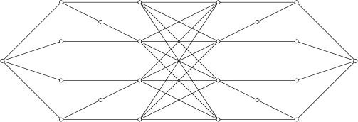
Figure 4.5: A graph in $\cal C$ with no extreme decomposition

So, we tried to prove that every triangle-free graph from $\cal C$ is 3-colorable directly by induction. To do this, we had to prove something stronger, and finding the right induction hypothesis had been quite painful. Let us call third color of a graph any stable set that contains at least one vertex of every odd cycle. Finding a third color is equivalent to 3-color a graph: give color 3 to the third color; since $G\setminus S$ contains no odd cycle, it is bipartite: color it with colors 1, 2.

Let us call strong third color of a graph any stable set that contains at least one vertex of every cycle (odd or even). Recall that $N[v]$ denotes $\{v\}\cup N(v)$. When $v$ is a vertex of a graph $G$, a pair of disjoint subsets $(R,T)$ of $V(G)$ is admissible with respect to $G$ and $v$ if one of the following holds (see Fig. 4.6):

• $T=N(v)$ and $R=\{v\}$;

• $T=\emptyset$ and $R=N[v]$;

• $v$ is of degree two, $N(v)=\{u,w\}$, $T=\{u\}$, $R=\{v,w\}$;

• $v$ is of degree two, $N(v)=\{u,w\}$, $T=\{u\}$, $R=N[w]$;

• $v$ is of degree two, $N(v)=\{u,w\}$, $T=\emptyset$, $R=\{u\}\cup N[w]$.

       

Figure 4.6: Five examples of admissible pairs (vertices of $T$ are white, vertices of $R$ are black)

We say that a pair of disjoint subsets $(R,T)$ is an admissible pair of $G$ if for some $v\in V(G)$, $(R,T)$ is admissible with respect to $G,v$. An admissible pair $(R,T)$ should be seen as a constraint for coloring: we will look for third colors (sometimes strong, sometimes not, we have to do this) that must contain every vertex of $T$ and no vertex of $R$. We do this first in basic graphs, and then by induction in all triangle-free graphs of $\cal C$, thus proving that they are 3-colorable. We give here the main statements but we omit the proofs.

Lemma 4.5

Let $G$ be a non-basic, connected, triangle-free, square-free and Petersen-free graph in $\cal C$ that has no 1-cutset and no proper 1-join. Let $(R,T)$ be an admissible pair of $G$. Then $G$ admits a strong third color $S$ such that $T\subseteq S$ and $S\cap R=\emptyset$.

In the proof of the lemma above we really need to find strong third colors for the sake of induction. But we cannot do this for all graphs in $\cal C$ because it is false in general that triangle-free graphs from $\cal C$ admit strong third colors. A counter-example is the graph $G$ obtained as follows: take four disjoint copies $\Pi_{1},\dots,\Pi_{4}$ of the Petersen graph minus one vertex. So $\Pi_{i}$ contains a set $X_{i}$ of three vertices of degree two ($i=1,\dots,4$). We add all edges between $X_{1},X_{2}$, between $X_{2},X_{3}$, between $X_{3},X_{4}$ and between $X_{4},X_{1}$. Note that $G$ can be obtained by gluing one square $S=s_{1}s_{2}s_{3}s_{4}$ and four disjoint copies of the Petersen graph along 1-joins, so it is a graph from $\cal C$.

We claim now that $G$ does not contain a stable set that intersects every cycle. Indeed, if $S$ is such a stable set then $S$ must contain all vertices in one of the $X_{i}$’s for otherwise we build a $C_{4}$ of $G\setminus S$ by choosing a vertex in every $X_{i}$. So $X_{1}\subseteq S$ say. We suppose that $\Pi_{1}$ has vertices $\{a_{2},\dots,a_{5},b_{1},\dots,b_{5}\}$ with our usual notation. So $X_{1}=\{b_{1},a_{2},a_{5}\}\subseteq S$ and we observe that every vertex in $C=V(\Pi_{1}\setminus S)$ has a neighbor in $X_{1}$. Hence $C\cap S=\emptyset$ while $G[C]$ is a cycle on six vertices, a contradiction.

Yet, we can prove that all graphs from $\cal C$ admit a third color.

Lemma 4.6

Let $G$ be a non-basic connected triangle-free graph in $\cal C$ and $(R,T)$ be an admissible pair of $G$. Then $G$ admits a third color $S$ such that $T\subseteq S$ and $S\cap R=\emptyset$.

All this shows that graphs in $\cal C$ have the best $\chi$-bounding function that one may expect for a class not included in perfect graphs: $f(2)=3$ and $f(x)=x$ for $x\geq 3$.

Theorem 4.7 (with Vušković [105])

Let $G$ be a graph that does not contain a cycle with a unique chord. Then either $\chi(G)=3$ or $\chi(G)=\omega(G)$.

The question of characterizing these graphs that are $\chi$-bounded with this function $f$ is widely open and Section 4.3 gives a conjecture about them.

4.2 Induced subdivision of $K_{4}$

Graphs with no subdivision of $K_{4}$ as a possibly non-induced subgraph are called series-parallel graphs. The structure of series-parallel graphs is well-known.

Theorem 4.8 (Duffin [40], Dirac [38])

Series-parallel graphs are graphs that arise from a forest by repeatedly applying the following operations:

• add a parallel edge to an existing edge and subdivide this new edge (this is the parallel extension);

• subdivide an edge (this is the series extension).

Exercise 4.9

Let $G$ be a 2-connected triangle-free series-parallel graph. Then either $G$ is isomorphic to $C_{4}$, to $C_{5}$ or to $K_{2,3}$, or $G$ contains at least 4 vertices of degree 2.

Of course, series-parallel graphs form an obvious basic class for ISK4-free graphs. So, an ISK4-free graph that is not basic should contain a subdivision $H$ of $K_{4}$ that has chords. Assuming that $H$ has a minimum number of vertex, we obtain the following. Recall that a wheel is obtained by taking a hole and adding a vertex with at least three neighbors in the hole.

Lemma 4.10 (with Lévêque and Maffray [69])

Let $G$ be an ISK4-free graph. Then either $G$ is a series-parallel graph, or $G$ contains a prism, or $G$ contains a wheel or $G$ contains $K_{3,3}$.

This lemma gives an obvious way to find a decomposition theorem for ISK4-free graphs: by proving attachment lemmas for prisms, wheels and $K_{3,3}$, and hoping that containing one of these entails a decomposition. The key question is the order in which the subgraphs should be considered. Hopefully, $K_{3,3}$ is quite easy. The following is not very difficult to prove.

Lemma 4.11 (with Lévêque and Maffray [69])

Let $G$ be an ISK4-free graph that contains $K_{3,3}$. Then either $G$ is a bipartite complete graph, or $G$ is a tripartite complete graph, or $G$ has a clique-cutset of size at most 3.

The Lemma above already gives us something. Since Scott’s Conjecture 2.3 is known to be true for $K_{3,3}$-free graphs by a theorem of Kühn and Osthus [66], we easily prove the following.

Theorem 4.12 (Scott [98])

${\rm Forb}^{*}(K_{4})$ is $\chi$-bounded.

The next question is to decide whether we should consider prisms or wheels first. Here, knowing a bit about Berge and claw-free graphs helps a lot to decide something (foolish or wise, but we have to decide). Because from them, we know that prisms are line-graphs that are likely to grow into bigger line-graphs while wheels are more messy. Indeed, if one attaches a vertex to a prism, it is very likely that a kind of pyramid (which is an ISK4) is created, there are only few exceptions to this and most of them actually give some bigger line-graphs. So, considering an inclusion-wise maximal induced subgraph isomorphic to a line-graph should give something. Note that the idea of considering a maximal line-graph in such a context is one of the key steps that lead to the proof of the Strong Perfect Graph Conjecture, but it was used before by Conforti and Cornuéjols [24].

Precise statements are postponed because we need long definitions. Let us say now that one attachment to a prism is pathological. Suppose that a prism contains a square and add a vertex complete to this square. This gives an ISK4-free graph, which is in fact a line-graph. But, add again another vertex complete to the same square. Then, no ISK4 is created, and the graph obtained is not a line-graph. So, some prisms are likely to grow in other directions than just line-graphs. It has been quite long to figure out that in fact, a single basic class arises from these pathological attachments, the so-called rich-squares. The smallest example of a rich-square is $L(K_{4})$, more famous as the octahedron. Even if it does not appear too much in the statements below, it behaves a bit as a sporadic ISK4-free graph.

Definitions

A separation of a graph $H$ is a pair $(A,B)$ of subsets of $V(H)$ such that $A\cup B=V(H)$ and there are no edges between $A\setminus B$ and $B\setminus A$. It is proper if both $A\setminus B$ and $B\setminus A$ are non-empty. The order of the separation is $|A\cap B|$. A $k$-separation is a separation $(A,B)$ such that $|A\cap B|\leq k$. A separation $(A,B)$ is cyclic if both $H[A]$ and $H[B]$ has cycles. A graph $H$ is cyclically 3-connected if it is 2-connected, not a cycle, and there is no cyclic 2-separation. Note that a cyclic 2-separation of any graph is proper. The reader might prefer to think about cyclically 3-connected graphs as follows.

Exercise 4.13

A graph $H$ is a cyclically 3-connected graph if and only if it is either a theta or a subdivision of a 3-connected graph.

Recall that a branch-vertex is a vertex of degree at least 3. A branch is a path whose ends are branch-vertices and whose interior vertices are not. A basic branch in a graph is branch such that no two vertices in it are members of a triangle. Note that a branch in a graph is either basic, or is an edge $uv$ and there is a common neighbor of $u,v$.

A triangular subdivision of $K_{4}$ is a subdivision of $K_{4}$ that contains a triangle. Note that a pyramid is a triangular ISK4. A square theta is a theta that contains a square. Rephrased: a theta with two branches of length two. A square prism is a prism that contains a square. Rephrased, a prism with two basic branches of length one. Rephrased again, the line-graph of a square theta. A square subdivision of $K_{4}$ is a subdivision of $K_{4}$ such that the four vertices of degree three in it lie in a possibly non-induced square. Rephrased: a subdivision of $K_{4}$ where only two edges with no common ends are possibly subdivided. An induced square in a graph is basic if an even number of edges in it lie in a triangle of the graph. It easily checked that the line-graph of a subdivision $H$ of $K_{4}$ contains a basic square if and only if $H$ is a square subdivision of $K_{4}$, and that the vertices in any basic square of $L(H)$ arise from the edges of a square on the branch-vertices of $H$. It is easily checked that a prism contains only basic squares.

If $X,Y$ are two basic branches of a graph $G$, a connection between $X$, $Y$ is a path $P=p\!-\!\cdots\!-\!p^{\prime}$ such that $p$ has neighbors in $X$, $p^{\prime}$ has neighbors in $Y$, no interior vertex of $P$ has neighbors in $X\cup Y$, and if $p\neq p^{\prime}$ then $p$ has no neighbor in $Y$ and $p^{\prime}$ has no neighbor in $X$.

When $S$ = $\{u_{1},u_{2},u_{3},u_{4}\}$ induces a square in a graph $G$ with $u_{1},u_{2},u_{3},u_{4}$ in this order along the square, a connection of $S$ is an induced path of $G$, no interior vertex of which has a neighbor in $S$, with ends $p,p^{\prime}$ such that either $p=p^{\prime}$ and $N_{S}(p)=S$; or $N_{S}(p)=\{u_{1},u_{2}\}$ and $N_{S}(p^{\prime})=\{u_{3},u_{4}\}$; or $N_{S}(p)=\{u_{1},u_{4}\}$ and $N_{S}(p^{\prime})=\{u_{2},u_{3}\}$.

The line-graph of $K_{4}$ is isomorphic to $K_{2,2,2}$. It is usually called the octahedron. It contains three basic squares. For every basic square $S$ of an octahedron $G$, the two vertices of $G\setminus S$ are both connexions of $S$. Note also that when $K$ is a square prism with a square $S$, then $V(K)\setminus S$ is a connection of $S$.

When $G$ is a graph, $H$ is a graph such that $L(H)$ is an induced subgraph of $G$, and $C$ is a connected induced subgraph of $V(G)\setminus L(H)$, we define several types that $C$ can have, according to its attachment over $L(H)$:

• $C$ is of type branch if the attachment of $C$ over $L(H)$ is included in a basic branch of $L(H)$;

• $C$ is of type triangle if the attachment of $C$ over $K$ is included in a triangle of $L(H)$;

• $C$ is of type augmenting if $C$ contains a connection $p\!-\!\cdots\!-\!p^{\prime}$ of two distinct basic branches $X,Y$ of $L(H)$, $N_{X}(p)$ is an edge of $X$ and $N_{Y}(p^{\prime})$ is an edge of $Y$. Moreover, there are no edges between $L(H)\setminus(X\cup Y)$ and $P$.

• $C$ is of type square if $L(H)$ contains a basic square $S$, and $C$ contains a connection $P$ of $S$. Moreover, there are no edges between $L(H)\setminus S$ and $P$.

Note that the types may overlap: a subgraph $C$ can be of more than one type. Since we view a vertex of $G$ as a connected induced subgraph of $G$, we may speak about the type of vertex with respect to $L(H)$.

Getting rid of prisms

Now the idea to decompose ISK4-free graphs further is the following: suppose that an ISK4-free graph $G$ contains a prism. So, $G$ contains a maximal line-graph $L(H)$. If there is nothing else in the graph, then $G$ itself is a line graph, so it is basic. Else, we are going to prove that any component $C$ of $G\setminus H$ is of one of the type defined above. Type branch gives a proper 2-cutset, type triangle gives a clique cutset and type augmenting gives a bigger line-graph, so a contradiction to the maximality of $L(H)$.

Type square is slightly more tricky. Sometimes, it gives a bigger line-graphs (when it is the only type square attachment to a given square). When used a second time, it often gives an ISK4, with two degenerate exceptions: when $L(H)$ is a square prisms or the line-graphs of a square subdivision of $K_{4}$. These two exceptions give the basic class of rich-squares: a rich square is a graph $K$ that contains a square $S$ as an induced subgraph, and such that $K\setminus S$ has at least two components and every component of $K\setminus S$ is a connection of $S$.

We give now the sequence of attachments lemmas that we need to show that when an ISK4-free graphs contains a prism then it is either basic or admits a decomposition. We give all the statements without proofs so that the readers feels the fun of trying to decompose a class, which is a bit like getting out of a maze. The slight problem is that trying a direction or another costs a lot of time, for instance, the proof of the Lemma 4.15 is 6 pages long despite efforts towards avoiding symmetric cases. But the next one is not so long and is a good exercise.

Lemma 4.14

Let $G$ be a graph that contains no triangular ISK4. Let $K$ be a prism that is an induced subgraph of $G$ and let $C$ be a connected induced subgraph of $G\setminus K$. Then $C$ is either of type branch, triangle, augmenting or square with respect to $K$.

Lemma 4.15

Let $G$ be a graph that contains no triangular ISK4. Let $H$ be a subdivision of $K_{4}$ such that $L(H)$ is an induced subgraph of $G$. Let $C$ be a connected induced subgraph of $G\setminus L(H)$. Then $C$ is either of type branch, triangle, augmenting or square with respect to $L(H)$.

A graph $H$ is substantial if it is cyclically 3-connected and neither a square theta nor a square subdivision of $K_{4}$. Note that in the next lemma, the type square is not needed.

Lemma 4.16

Let $G$ be a graph that contains no triangular ISK4. Let $H$ be a substantial graph such that $L(H)$ is an induced subgraph of $G$. Let $C$ be a component of $G\setminus L(H)$. Then $C$ is either of type branch, triangle or augmenting with respect to $L(H)$.

The next lemmas are not attachment lemmas, but decomposition results that use the lemmas above.

Lemma 4.17

Let $G$ be a graph that contains no triangular ISK4. Let $H$ be a substantial graph such that $L(H)$ is an induced subgraph of $G$. Suppose $L(H)$ inclusion-wise maximum with respect to that property.

Then either $G=L(H)$ or $G$ has a clique-cutset of size at most three, or $G$ has a proper 2-cutset.

The next two lemmas sort out which prisms give line-graphs and which prisms give rich-squares.

Lemma 4.18

Let $G$ be an ISK4-free graph that contains no line-graph of a substantial graph. Let $K$ be a rich square that is an induced subgraph of $G$, and maximal with respect to this property. Then either $G=K$ or $G$ has a clique-cutset of size at most three or $G$ has a proper 2-cutset.

Lemma 4.19

Let $G$ be an ISK4-free graph that contains no line-graph of a substantial graph and no rich square as an induced subgraph. Let $K$ be a prism that is an induced subgraph of $G$. Then either $G=K$ or $G$ has a clique-cutset of size at most three or $G$ has a proper 2-cutset.

The next theorem was our goal. It is easy to prove with all the lemmas above. Thanks to it, we “get rid of prisms”.

Theorem 4.20 (with Lévêque and Maffray [69])

Let $G$ be an ISK4-free graph that contains a prism or an octahedron. Then either $G$ is the line-graph of a graph with maximum degree three, or $G$ is a rich square, or $G$ has a clique-cutset of size at most three or $G$ has a proper 2-cutset.

Getting rid of wheels

In view of Lemma 4.10, our next to goal is to produce something like Theorem 4.20 with “wheel” instead of “prism”. The only result we could prove is the following.

A double star cutset of a graph is a set $S$ of vertices such that $G\setminus S$ is disconnected and such that $S$ contains two vertices $u,v$ and every vertex of $G$ is adjacent at least one of $u,v$. In particular $u$ and $v$ are adjacent. Note that a star-cutset is either a double star cutset or consists of one vertex.

Lemma 4.21 (with Lévêque and Maffray [69])

Let $G$ be an ISK4-free graph that does not contain a prism or an octahedron. If $G$ contains a wheel, then $G$ has a star-cutset or a double star cutset.

Thanks to the lemma above, we can easily devise a decomposition theorem for ISK4-free graphs that uses double-star cutsets, but I do not want even to state this here because it is useless. These double star cutsets are strong cutsets. In some situations, they are very useful: they are the best known cutsets for odd hole-free graphs (Theorem 5.1) and they are used by Cornuéjols, Liu and Vušković [13] to give an interesting recognition algorithm of Berge graphs based on decomposition. But from a bunch examples, we feel that ISK4-free graphs should be decomposable with better cutsets, as star cutset or perhaps 3-cutsets. This research is still in progress. We are not very optimistic for the recognition algorithm, but we hope to prove the following.

Conjecture 4.22

Any ISK4-free graph is 4-colorable.

4.3 Graphs with no wheels

The previous section suggests that wheels are annoying. Also in the original proof of the Strong Perfect Graph Theorem, the most difficult part was devoted to wheel systems, a very complicated construction to decompose a Berge graph containing a wheel. So, perhaps nice things happen if we exclude wheels? Indeed, from the lemmas in the section above, we obtain easily a very precise decomposition theorem.

Theorem 4.23 (with Lévêque and Maffray [69])

Let $G$ be an ISK4-free graph with no wheel. Then either:

• $G$ is series-parallel;

• $G$ is the line-graph of a graph with maximum degree three;

• $G$ is a rich square;

• $G$ is a complete bipartite graph;

• $G$ is a complete tripartite graph;

• $G$ has a clique-cutset of size at most three;

• $G$ has a proper 2-cutset.

In several simple classes, we also obtain results.

Lemma 4.24 (with Lévêque and Maffray [69])

Let $G$ be a rich square that contains no wheel. Then $G$ is $3$-colorable.

It is easy to check that a line-graph $G=L(R)$ contains a wheels if and only if $R$ contains a cycle with at least one chord. So, a line-graph with no wheel is the line-graph of a chordless graph. In fact, with Lévêque and Maffray this was our motivation to study chordless graphs, and it was lucky that a few months before they were studied implicitly in the paper [105] with Vušković on cycles with a unique chord. From this remark and Theorem 2.16 we get the following.

Lemma 4.25 (with Lévêque and Maffray [69])

Let $G$ be a graph that contains no ISK4, no wheel and such that $G$ is a line-graph. Then $G$ is $3$-colorable.

Exercise 4.26

Prove or disprove that for all line-graphs $G$ with no wheel $\chi(G)=3$ or $\chi(G)=\omega(G)$.

Finally, by combining all the results above, we obtain the following.

Theorem 4.27 (with Lévêque and Maffray [69])

Let $G$ be a graph that contains no ISK4 and no wheel. Then $G$ is $3$-colorable.

This suggests that some bounds on $\chi$ could be obtained for graphs with no wheels. We have no counter-example to the following.

Conjecture 4.28 (with Lévêque and Maffray [69])

A graph $G$ with no wheel satisfies $\chi(G)=3$ or $\chi(G)=\omega(G)$.

In fact, a wheel always contains a cycle with a unique chord. So, Theorem 4.7 is a weaker form of the conjecture. The following also could be a not so difficult weaker form.

Question 4.29

A planar graph with no wheel as a subgraph (possibly non-induced) admits a vertex of degree at most 2.

The following is certainly very difficult and Theorems 4.1 and 4.23 can be seen as weaker forms of an answer to it.

Question 4.30

Find a decomposition theorem for wheel-free graphs.

Chapter 5 Berge graphs

Berge graphs is perhaps the most studied class of graphs closed under taking induced subgraphs, especially if one takes into account that many works on other classes are motivated by their inclusion in Berge graphs. Writing a survey about Berge graphs is uncomfortable because a long list of definitions is needed just to state the results. If these definitions are skipped, the survey becomes fuzzy. Let us try both approaches by keeping the fuzziness for this short introduction and postponing the formal definitions to the next section.

In the eighties, the idea of proving the Strong Perfect Graph Conjecture by decomposing Berge graphs started to be advocated by researchers around Vašek Chvátal. During a talk given in July 2004 at the conference held in Paris honoring the memory of Claude Berge, Chvátal said that as far as he remembered, Sue Whitesides was the first researcher who told him about that. Guessing the right decomposition statement has been a long process. Inventing operations that preserve perfectness started from the very beginning of the study of perfect graphs with the clique cutset, continued with Lovász’ replication of vertices, Fonlupt and Urhy’s contraction of even pairs, Burlet and Fonlupt’s amalgam and finally Cornuéjols and Cunningham’s 2-join and Chvátal and Sbihi’s homogeneous pair. But keeping the focus on these operations means in fact looking for a structure theorem. So, a key step toward a more realistic decomposition statement applying to all Berge graphs was the introduction of strong cutsets by Chvátal: star cutsets and skew partitions. So, at the end of the eighties, most of the ingredients to state a decomposition theorem for Berge graphs were present. But as any cooker knows, having the ingredients does not mean having your dinner ready.

Interesting attempts to state reasonable decomposition theorems were done by Bruce Reed and later disproved by Irena Rusu. All this is explained in the introduction of [15]. Finally, what seems today to be the good statement was guessed around 2000 by Michele Conforti, Gérard Cornuéjols and Kristina Vušković. Thanks to their experience on the decomposition of balanced matrices (arising from integer programming), they had a good intuition of what was going on. But more than just guessing the statement, they provided realistic plans toward a proof: a thorough study of a similar class (even-hole-free graphs, that they studied with Ajai Kapoor) and a serie of papers proving special cases of the Strong Perfect Graph Conjecture. These papers give an extremely useful tool-box: attachment to prisms, how to deal with line-graphs, attempts to use the cleaning which lead naturally to Roussel-and-Rubio-like lemmas… Also, they point out a theorem of Truemper on signing the edges of a graph and the related key-role played by the Truemper configurations which are 3PC’s (a.k.a. prisms, pyramids and thetas) and wheels. All this culminated with a decomposition theorem for square-free Berge graphs and a decomposition theorem for odd-hole-free graphs, that does not imply the Strong Perfect Graph Conjecture but is interesting in its own right.

The methods used in the group of Gérard Cornuéjols were precisely the kind of things where the group around Paul Seymour was very good at. So, it was natural for him to try to decompose Berge graphs. Robertson and Seymour got a grant for that (this story is interesting, see [100]), and they were joined by Robin Thomas and later Maria Chudnovsky. Finally, thanks to an impressive list of brilliant technicalities (found in only 2 years) and after a very long proof, they could settle the Strong Perfect Graph Conjecture in May 2002. The decomposition theorem of Chudnovsky et al. states that every Berge graph is either basic or decomposable. Here basic means bipartite, line-graph of bipartite, or complement of these. There is another class, double split graphs, whose definition is postponed to the next section. Decomposable means having a 2-join, a homogeneous pair or a balanced skew partition. A balanced skew partition is a skew partition with parity constraints on the paths and antipaths linking the different boxes of the partition. Note that all basic classes are really basic for many questions. In particular, they are easy to recognize and fast algorithms exist to optimize them. The 2-join and the homogeneous pairs are known to be good decompositions, in the sense that they are reversible and possibly useful for optimization algorithms. But as the sequel will show, very few researches are devoted to optimize with them. In contrast, so far, no one seems to know how skew partitions (balanced or not) could be used in optimization algorithms.

Let me now explain how the work I did takes place in the story summed up above. I did my thesis in 2001–2004, during the exciting time where all these results were presented in several conferences that I was lucky to attend to. I was lucky also to be supervised by Frédéric Maffray who had a broad knowledge of perfect graphs and spent hours passing it on to me. He was wise enough to be confident that structural methods could finally settle the Conjecture; he experienced this himself by proving a structural description of claw-free perfect graphs [77]. So, he was paying a very careful attention to the work done in the two leading teams. In the same time, he was trying to use even pairs and in November 2002, during the conference on perfect graphs of Palo Alto, we could prove together the existence of even pairs in Artemis graphs, something conjectured by Hazel Everett and Bruce Reed. Our method was something Maffray already used with Cláudia Linhares Sales for square-free Artemis graphs, and what we did was using Roussel-and-Rubio-like lemmas to handle squares. The same method has been used recently by Chudnovsky and Seymour to shorten the proof of the Strong Perfect Graph Theorem.

This was nice, but at the end of my thesis, I had a little problem: how to find a good research direction in such a field and after all this? Giving up perfect graphs and doing something else was an option, but after spending so many hours reading difficult papers, I felt it would be a kind of waste. Pushing further the method that worked for Artemis graphs was something we already tried quite hard with Maffray. The last important open question on perfect graphs, coloring them by a combinatorial algorithm, was too difficult. Among the list of outcomes of the decomposition theorem for Berge graphs, all were testable in polynomial time except one: the presence of a balanced skew partition. But there was a polynomial time algorithm for skew partition (balanced or not) due to de Figueiredo, Klein, Kohayakawa and Reed. Also, algorithms for partitioning graphs into boxes with prescribed adjacencies in various ways was a subject with interesting recent progress, see for instance [41]. So, the detection of balanced skew partitions seemed to be a problem of reasonable interest and difficulty.

The obvious way to attack the problem was to see how the people working on the partition of vertices into boxes solve their problems, and then see how to handle the “balanced” constraint on the parity of paths. But this was likely to be a dead end (or to be too difficult), because the main result of the paper of Bienstock [6] is that deciding whether there exists a path of odd length between two given vertices of a graph is NP-complete. So, it was clear to me that detecting balanced skew partitions should be NP-hard, and indeed, it is easy to prove this with Bienstock’s construction, see Theorem 5.5.

After attending a talk of Celina de Figueiredo in Grenoble (in June 2004), I realised that the problem could be solved by decomposition methods for Berge graphs. If the graph is basic, there is a hope to detect balanced skew partitions directly. If the graph has a 2-join, there is a hope to decompose and to solve the question recursively. If a graph is not basic and has no 2-join, just answer “there is a balanced skew partition”, the correct answer because of a theorem of Chudnovsky stating that homogeneous pairs are in fact useless to decompose Berge graphs. This blind use of decomposition is a kind of cheating, but is formally correct. All this could have been easy, and I was planning to write something short about that. But it was more difficult than expected. Building the blocks of a 2-join in the usual way does not preserve balanced skew partitions because of the so-called path 2-joins; this issue and how to bypass it is explained Section 5.2. Finally, a structure theorem for graphs with no balanced skew partitions was needed and resulted into 50 pages of proof sketched in Section 5.3. The detection of balanced skew partition in Berge graphs was solved but the intermediate structure theorem to solve it was more interesting than the result itself.

A natural next step was trying to use the structure theorem to optimize Berge graphs with no balanced skew partitions. I tried alone, with Gautier Stauffer, with Sulamita Klein and discussed this a bit with Maffray and Vušković. But all these attempts failed. I discussed this again in November 2008 in Rio, with Simone Dantas, Sulamita Klein and Celina de Figueiredo. I explained them that homogeneous pairs were in fact a problem despite the theorem of Chudnovsky. Then, Celina suggested to work on Berge graphs with no balanced skew partitions and no homogeneous pairs. This was a very good hint, since with Vušković we could in fact color these graphs, see Sections 5.4 devoted to the structure of the class, 5.5 devoted to the computation of maximum cliques and stable set, and 5.6 devoted to coloring the class.

Before explaining all this, let me say that I am grateful to Celina de Figueiredo because she gave me good hints for the two papers I wrote on decomposing Berge graphs.

5.1 Decomposing Berge graphs: main results

Skew partitions were first introduced by Chvátal [22]. A complete pair in a graph is a pair $(A,B)$ made of two disjoint sets of vertices with all possible edges between them. An anticomplete pair is a pair that is complete in the complement of the graph. A skew partition of a graph $G=(V,E)$ is a partition of $V$ into two sets $A$ and $B$ such that $A$ induces a graph that is not connected, and $B$ induces a graph that is not anticonnected. When $A_{1},A_{2},B_{1},B_{2}$ are non-empty sets such that $(A_{1},A_{2})$ partitions $A$, $(A_{1},A_{2})$ is an anticomplete pair, $(B_{1},B_{2})$ partitions $B$, and ($B_{1},B_{2}$) is a complete pair, we say that $(A_{1},A_{2},B_{1},B_{2})$ is a split of the skew partition $(A,B)$. A balanced skew partition (first defined in [15]) is a skew partition $(A,B)$ with the additional property that every induced path of length at least 2 with ends in $B$, interior in $A$ has even length, and every antipath of length at least 2 with ends in $A$, interior in $B$ has even length. If $(A,B)$ is a skew partition, we say that $B$ is a skew cutset. If $(A,B)$ is balanced we say that the skew cutset $B$ is balanced. Note that Chudnovsky et al. [15] proved that no minimum counter-example to the strong perfect graph conjecture has a balanced skew partition.

Call double split graph (first defined in [15]) any graph $G$ that can be constructed as follows. Let $m,n\geq 2$ be integers. Let $A=\{a_{1},\dots,a_{m}\}$, $B=\{b_{1},\dots,b_{m}\}$, $C=\{c_{1},\dots,c_{n}\}$, $D=\{d_{1},\dots,d_{n}\}$ be four disjoint sets. Let $G$ have vertex set $A\cup B\cup C\cup D$ and edges in such a way that:

• $a_{i}$ is adjacent to $b_{i}$ for $1\leq i\leq m$. There are no edges between $\{a_{i},b_{i}\}$ and $\{a_{i^{\prime}},b_{i^{\prime}}\}$ for $1\leq i<i^{\prime}\leq m$;

• $c_{j}$ is non-adjacent to $d_{j}$ for $1\leq j\leq n$. There are all four edges between $\{c_{j},d_{j}\}$ and $\{c_{j^{\prime}},b_{j^{\prime}}\}$ for $1\leq j<j^{\prime}\leq n$;

• there are exactly two edges between $\{a_{i},b_{i}\}$ and $\{c_{j},d_{j}\}$ for $1\leq i\leq m$, $1\leq j\leq n$ and these two edges are disjoint.

Note that $C\cup D$ is a non-balanced skew cutset of $G$ and that $\overline{G}$ is a double split graph. Note that in a double split graph, vertices in $A\cup B$ all have degree $n+1$ and vertices in $C\cup D$ all have degree $2n+m-2$. Since $n\geq 2,m\geq 2$ implies $2n-2+m>1+n$, it is clear that given a double split graph the partition $(A\cup B,C\cup D)$ is unique.

A graph is said to be basic if one of $G,\overline{G}$ is either a bipartite graph, the line-graph of a bipartite graph or a double split graph.

The 2-join was first defined by Cornuéjols and Cunningham [32]. A partition $(X_{1},X_{2})$ of the vertex set is a 2-join when there exist disjoint non-empty $A_{i},B_{i}\subseteq X_{i}$ ($i=1,2$) satisfying:

• every vertex of $A_{1}$ is adjacent to every vertex of $A_{2}$ and every vertex of $B_{1}$ is adjacent to every vertex of $B_{2}$;

• there are no other edges between $X_{1}$ and $X_{2}$.

The sets $X_{1},X_{2}$ are the two sides of the 2-join. When sets $A_{i}$’s $B_{i}$’s are like in the definition we say that $(X_{1},X_{2},A_{1},B_{1},A_{2},B_{2})$ is a split of $(X_{1},X_{2})$. Implicitly, for $i=1,2$, we will denote by $C_{i}$ the set $X_{i}\setminus(A_{i}\cup B_{i})$.

A 2-join $(X_{1},X_{2})$ in a graph $G$ is said to be connected when for $i=1,2$, every component of $G[X_{i}]$ meets both $A_{i}$ and $B_{i}$. A 2-join $(X_{1},X_{2})$ is said to be substantial when for $i=1,2$, $|X_{i}|\geq 3$ and $X_{i}$ is not a path of length 2 with an end in $A_{i}$, an end in $B_{i}$ and its unique interior vertex in $C_{i}$. A 2-join $(X_{1},X_{2})$ in a graph $G$ is said to be proper when it is connected and substantial.

A 2-join is said to be a path 2-join if it has a split $(X_{1},X_{2},A_{1},B_{1},A_{2},B_{2})$ such that $G[X_{1}]$ is a path with an end in $A_{1}$, an end in $B_{1}$ and interior in $C_{1}$. Implicitly we will then denote by $a_{1}$ the unique vertex in $A_{1}$ and by $b_{1}$ the unique vertex in $B_{1}$. We say that $X_{1}$ is the path-side of the 2-join. Note that when $G$ is not a hole then only one of $X_{1},X_{2}$ is a path side of $(X_{1},X_{2})$. A non-path 2-join is a 2-join that is not a path 2-join.

The homogeneous pair was first defined by Chvátal and Sbihi [23]. The definition that we give here is a slight variation used in [15]. A homogeneous pair is a partition of $V(G)$ into six non-empty sets $(A,B,C,D,E,F)$ such that:

• every vertex in $A$ has a neighbor in $B$ and a non-neighbor in $B$, and vice versa;

• the pairs $(C,A)$, $(A,F)$, $(F,B)$, $(B,D)$ are complete;

• the pairs $(D,A)$, $(A,E)$, $(E,B)$, $(B,C)$ are anticomplete.

A graph $G$ is path-cobipartite if it is a Berge graph obtained by subdividing an edge between the two cliques that partitions a cobipartite graph. More precisely, a graph is path-cobipartite if its vertex set can be partitioned into three sets $A,B,P$ where $A$ and $B$ are non-empty cliques and $P$ consists of vertices of degree 2, each of which belongs to the interior of a unique path of odd length with one end $a$ in $A$, the other one $b$ in $B$. Moreover, $a$ has neighbors only in $A\cup P$ and $b$ has neighbors only in $B\cup P$. Note that a path-cobipartite graph such that $P$ is empty is the complement of bipartite graph. Note that our path-cobipartite graphs are simply the complement of the path-bipartite graphs defined by Chudnovsky in [11]. For convenience, we prefer to think about them in the complement as we do.

A double star in a graph is a subset $D$ of the vertices such that there is an edge $ab$ in $G[D]$ satisfying: $D\subset N(a)\cup N(b)$.

Now we can state the known decomposition theorems of Berge graphs. The first decomposition theorem for Berge graph ever proved is the following:

Theorem 5.1 (Conforti, Cornuéjols and Vušković, 2001, [28])

Every graph with no odd hole is either basic or has a proper 2-join or has a double star cutset.

It could be thought that this theorem is useless to prove the Strong Perfect Graph Theorem since there are minimal imperfect graphs that have double star cutsets: the odd antiholes of length at least 7. However, by the Strong Perfect Graph Theorem, we know that the following fact is true: for any minimal non-perfect graph $G$, one of $G,\overline{G}$ has no double star cutset. A direct proof of this — of which we have no idea — would yield together with Theorem 5.1 a new proof of the Strong Perfect Graph Theorem.

The following theorem was first conjectured in a slightly different form by Conforti, Cornuéjols and Vušković, who proved it in the particular case of square-free graphs [27]. A corollary of it is the Strong Perfect Graph Theorem.

Theorem 5.2 (Chudnovsky, Robertson, Seymour and Thomas, 2002, [15])

Let $G$ be a Berge graph. Then either $G$ is basic or $G$ has a homogeneous pair, or $G$ has a  balanced  skew partition or one of $G,\overline{G}$ has a proper 2-join.

The two theorems that we state now are due to Chudnovsky who proved them from scratch, that is without assuming Theorem 5.2. Her proof uses the notion of trigraph. The first theorem shows that homogeneous pairs are not necessary to decompose Berge graphs. Thus it is a result stronger than Theorem 5.2. The second one shows that path 2-joins are not necessary to decompose Berge graphs, but at the expense of extending balanced skew partitions to general skew partitions and introducing a new basic class. Note that a third theorem can be obtained by viewing the second one in the complement of $G$.

Theorem 5.3 (Chudnovsky, 2003, [12, 11])

Let $G$ be a Berge graph. Then either $G$ is basic, or one of $G,\overline{G}$ has a proper 2-join or $G$ has a  balanced  skew partition.

Theorem 5.4 (Chudnovsky, 2003, [11])

Let $G$ be a Berge graph. Then either $G$ is basic, or one of $G,\overline{G}$ is path-bipartite, or $G$ has a proper non-path 2-join, or $\overline{G}$ has a proper 2-join, or $G$ has a homogeneous pair or $G$ has a skew partition.

5.2 Detection of balanced skew partitions

Before explaining Theorem 5.10, a new decomposition for Berge graphs that is a generalization of Theorems 5.2, 5.3 and 5.4, let us explain its initial motivation: the detection of balanced skew partitions. De Figueiredo, Klein, Kohayakawa and Reed devised an algorithm that given a graph $G$ computes in polynomial time a skew partition if $G$ has one [36]. See also a recent work by Kennedy and Reed [62]. Let us call BSP the decision problem whose input is a graph and whose answer is YES if the graph has a balanced skew partition and NO otherwise. Using a construction due to Bienstock [6], we can prove the following.

Theorem 5.5 ([104])

BSP is NP-hard.

Note that we are not able to prove that BSP is in NP or in coNP. But using Theorem 5.10, we give an $O(n^{9})$-time algorithm for BSP restricted to Berge graphs. Let us explain how.

In 2002, Chudnovsky, Cornuéjols, Liu, Seymour and Vušković [13] gave an algorithm that recognizes Berge graphs in time $O(n^{9})$. This algorithm may be used to prove that, when restricted to Berge graphs, BSP is in NP. Indeed, a  balanced  skew partition is a good certificate for BSP: given a Berge graph and a partition $(A,B)$ of its vertices, one can easily check that $(A,B)$ is a skew partition; to check that it is balanced, it suffices to add a vertex adjacent to every vertex of $B$, to no vertex of $A$, and to check that this new graph is still Berge.

Proving that BSP is actually in P by a decomposition theorem uses a classical idea, used for instance in [26] to check whether a given graph has or not an even hole. First, solve BSP for each class of basic graph. This can be done in time $O(n^{5})$. Note that bipartite graphs are the most difficult to handle efficiently. For them, we use an algorithm due to Reed [95] for general skew partitions; and since balanced and general skew partitions are the same thing in bipartite graphs (see below), an algorithm follows.

Lemma 5.6 ([104])

Let $G$ be a bipartite graph. Then $(A,B)$ is a skew partition of $G$ if and only if it is a balanced skew partition of $G$.

The following two lemmas show how to handle the other basic classes. Note that the balanced skew partition is a self-complementary notion, so the complements of the classes need no special treatment.

Lemma 5.7 ([104])

A double split graph $G$ has exactly one skew partition and this skew partition is not balanced.

Lemma 5.8 ([104])

Let $G$ be the line-graph of a bipartite graph. Suppose that $G$ has at least one edge and at least 5 vertices. Then $G$ has a  balanced  skew partition if and only if $G$ has a star cutset.

For a graph $G$ such that one of $G,\overline{G}$ has a 2-join, we try to break $G$ into smaller blocks in such a way that $G$ has a balanced skew partition if and only if one of the blocks has one, allowing us to run recursively the algorithm. And when a graph is not basic and has no 2-join, we simply answer “the graph has a balanced skew partition”, which is the correct answer because of the Decomposition Theorem 5.3. This blind use of decomposition is not safe from criticism, but this will be discussed later.

Let us now explain why without further work, this idea fails to solve BSP. Building the blocks of a 2-join preserves existing balanced skew partitions, but some 2-joins can create balanced skew partitions when building the blocks carelessly. For non-path 2-join, there is no problem: sides of the 2-join can be replaced safely by sufficiently long paths. But for path 2-joins, there is a problem. In the graph represented in Fig. 5.1 on the left, we have to simplify somehow the left part of the obvious path 2-join to build one of the blocks. The most reasonable way to do so seems to be replacing $X_{1}$ by a path of length 1. But this creates a skew cutset: the black vertices on the right. Of course, this graph is bipartite but one can find more complicated examples based on the same template, and another template exists. These bad 2-joins will be described in more details in Section 5.3 and called cutting 2-joins. All of them are path 2-joins.

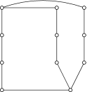
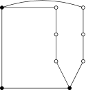
Figure 5.1: Contracting a path creates a skew cutset

Theorem 5.10 shows that cutting 2-joins are not necessary to decompose Berge graphs. A more general statement is proved, that makes use of a new basic class and of a new kind of decomposition that are quite long to describe. But an interesting corollary can be stated with no new notions. By contracting a path $P$ that is the side of a proper path 2-join of a graph we mean delete the interior vertices of $P$, and link the ends of $P$ with a path of length 1 or 2 according to the original parity of the length of $P$.

Theorem 5.9 ([104])

Let $G$ be a Berge graph. Then either:

• $G$ is basic;

• one of $G,\overline{G}$ has a non-path proper 2-join;

• $G$ has no balanced skew partition and exactly one of $G,\overline{G}$ (say $G$) has a proper path 2-join. Moreover, for every proper path 2-join of $G$, the graph obtained by contracting its path-side has no balanced skew partition;

• $G$ has a  balanced  skew partition.

The algorithm for detecting balanced skew partitions is now easy to sketch. Since the balanced skew partition is a self-complementary notion, we may switch from the graph to its complement as often as needed. First check whether the input graph is basic, and if so look directly for a balanced skew partition. Else, try to decompose along non-path 2-joins (they preserve the existence of balanced skew partitions). If there are none of them, try to decompose along path 2-joins (possibly, this creates balanced skew partitions but does not destroy them). At the end of this process, one of the leaves of the decomposition tree has a balanced skew partition if and only if the root has one. Note that a balanced skew partition in a leaf may have been created by the contraction of a cutting 2-join since such 2-joins do exist (we are not able to recognize all of them, it seems to be a difficult task). But Theorem 5.9 shows that when such a bad contraction occurs, the graph has anyway a balanced skew cutset somewhere.

All this runs in time $O(n^{9})$. The complexity is the same as the recognition of Berge graphs but this is purely coincidental. The complexity bottleneck of our algorithm is the routine to search for a non-path 2-join. This takes $O(n^{8})$, and speed it up to $O(n^{5})$ would speed up the algorithm. Speed it up further would be useless because of the second bottleneck which is detecting a skew partition in a bipartite graph in time $O(n^{5})$.

Let us come back to the weak point of our recognition algorithm, which is when it answers “the graph has a balanced skew-partition” using blindly some decomposition theorem. This weakness is the reason why we are not able to find explicitly a balanced skew partition when there is one. However, our result suggests that an explicit algorithm might exist. The proof of Theorem 5.2 or Theorem 5.3 might contain its main steps. However, we would like to point out that if someone manage to read algorithmically the proof of Theorem 5.2 or of Theorem 5.3, (s)he will probably end up with an algorithm that given a graph, either finds an odd hole/antihole, or certifies that the graph is basic, or finds some decomposition. If the decomposition found is not a balanced skew partition, the algorithm will probably not certify that there is no balanced skew partition in the graph, and thus BSP will not be solved entirely. To solve it, one will have to think about the detection of balanced skew partitions in basic graphs, and in graphs having a 2-join: this is what we are doing here. Thus an effective algorithm might have to use much of the present work.

5.3 A new decomposition theorem for Berge graphs

As stated in Section 5.2, our main problem for the detection of balanced skew partitions is the possibility of path 2-joins in Berge graphs. One could hope that these 2-joins are actually not necessary to decompose Berge graphs. Theorem 5.4 indicates that such a hope is realistic, but this theorem allows non-balanced skew partitions, so it is useless for our purpose. What we would like is to prove something like Theorem 5.3 with “non-path 2-join” instead of “2-join”. Let us call this statement our conjecture. A simple idea to prove the conjecture would be to consider a minimum counter-example $G$, that is: a Berge graph, non-basic, with no balanced skew partition, and no non-path 2-join. Such a graph must have a path 2-join by Theorem 5.3 (possibly after taking the complement). Here is why we need Theorem 5.3 in our proof. The idea is now to use this path 2-join to build a smaller graph $G^{\prime}$ that is also a counter-example, and this is a contradiction which proves the conjecture.

So, given $G$ with its path 2-join, how can we build a smaller graph that will have “almost” the same structure as $G$ ? Obviously, this can be done by contracting the path-side of the 2-join. Let us call $G_{c}$ the graph that we obtain. It has to be proved that $G_{c}$ is still a counter-example to the conjecture. But we know that this can be false. Indeed, if the path 2-join of $G$ is cutting, a balanced skew partition can be created in $G_{c}$, so $G_{c}$ is not a counter-example. We need now to be more specific and to define cutting 2-joins.

$G$	$G_{c}$	$G^{\prime}$

Figure 5.2: A graph $G$ with a cutting 2-join of type 1 and the associated graph $G^{\prime}$

A 2-join is said to be cutting of type 1 if it has a split $(X_{1},$ $X_{2},$ $A_{1},$ $B_{1},$ $A_{2},$ $B_{2})$ such that:

1. $(X_{1},X_{2})$ is a path 2-join with path-side $X_{1}$;

2. $G[X_{2}\setminus A_{2}]$ is disconnected.

In Fig. 5.2 the structure of a graph $G$ with a cutting 2-join of type 1 is represented. Obviously, after contracting the path-side into an edge $a_{1}b_{1}$, we obtain a graph $G_{c}$ with a potentially-balanced skew cutset $\{a_{1},b_{1}\}\cup A_{2}$ that separates $C_{3}\cup B_{3}$ from $C_{4}\cup B_{4}$. So, how can we find a graph smaller than $G$ that is still a counter-example to the conjecture? Our idea is to build the graph $G^{\prime}$, also represented in Fig. 5.2. If we count vertices, $G^{\prime}$ is not “smaller” than $G$, but in fact, by “minimum counter-example” we mean counter-example with a minimum number of path 2-joins. We can prove that $G^{\prime}$ is smaller in this sense (this is not trivial because we have to prove that path 2-joins cannot be created in $G^{\prime}$, but clearly, one path 2-join is destroyed in $G^{\prime}$). We can also prove that $G^{\prime}$ is a counter-example which gives the desired contradiction. This is the first case of the proof of Theorem 5.10. Note that finding the right graph $G^{\prime}$ has been long and painful (in particular the strange little hat $b_{1}$ that is so useful). But once $G^{\prime}$ is found, the proof is not really difficult. Yet, it is quite long (about 10 pages) and relies on many easy lemmas on parities of various paths and antipaths. Proving that $G^{\prime}$ has no non-path 2-join is the main difficulty and is very tedious. A good exercise is to prove that $G^{\prime}$ is Berge.

$G$	$G_{c}$	$G^{\prime}$

Figure 5.3: A graph $G$ with a cutting 2-join of type 2 and the associated graph $G^{\prime}$

Unfortunately, there is another kind of path 2-join that can create balanced skew partitions when contracting the path-side. A 2-join is said to be cutting of type 2 if it has a split $(X_{1},$ $X_{2},$ $A_{1},$ $B_{1},$ $A_{2},$ $B_{2})$ such that there exist sets $A_{3}$, $B_{3}$ satisfying:

1. $(X_{1},X_{2})$ is a path 2-join with path-side $X_{1}$;

2. $A_{3}\neq\emptyset$, $B_{3}\neq\emptyset$, $A_{3}\subset A_{2}$, $B_{3}\subset B_{2}$;

3. $A_{3}$ is complete to $B_{3}$;

4. every outgoing path from $B_{3}\cup\{a_{1}\}$ to $B_{3}\cup\{a_{1}\}$ (resp. from $A_{3}\cup\{b_{1}\}$ to $A_{3}\cup\{b_{1}\}$) has even length;

5. every antipath of length at least 2 with its ends outside $B_{3}\cup\{a_{1}\}$ (resp. $A_{3}\cup\{b_{1}\}$) and its interior in $B_{3}\cup\{a_{1}\}$ (resp. $A_{3}\cup\{b_{1}\}$) has even length;

6. $G\setminus(X_{1}\cup A_{3}\cup B_{3})$ is disconnected.

In Fig. 5.3, the structure of a graph $G$ with a cutting 2-join of type 2 is represented. After contracting the path-side into an edge $a_{1}b_{1}$, we obtain a graph $G_{c}$ with a balanced skew cutset $\{a_{1},b_{1}\}\cup A_{3}\cup B_{3}$. It is “skew” because $a_{1}\cup B_{3}$ is complete to $b_{1}\cup A_{3}$, and it is balanced by the parity constraints in the definition. How can we find a graph smaller than $G$ that is still a counter-example to the conjecture ? Again, we find a graph $G^{\prime}$, also represented in Fig. 5.3. Again, we prove that $G^{\prime}$ is a smaller counter-example, a contradiction. This is the second case of the proof of Theorem 5.10.

Note that we are not able to prove something like Theorem 5.9 with “skew partition” instead of “balanced skew partition”. Following our frame, we would have to give up the conditions on the parity of paths in the definition of cutting 2-joins of type 2. But then we would not be able to prove that $G^{\prime}$ is Berge, making the whole proof collapse. Also we would like to explain a little twist in our proof. In fact Case 2 is not “the 2-join is cutting of type 2”, but something slightly more general: “the 2-join is such that there are sets $A_{3}$, $B_{3}$ satisfying the items 1–5 of the definition of cutting 2-joins of type 2”. Indeed, in Case 2, we do not need to use the last item. And this has to be done, since in Case 3, at some place where we need a contradiction, we find a 2-join that is almost of type 2, that satisfies items 1–5, and not the last one.

A 2-join is said to be cutting if it is either cutting of type 1 or cutting of type 2. So, in our main proof we can get rid of cutting 2-joins as explained above. In [104], we also study how a 2-join and a balanced skew partition can overlap in a Berge graph. The main result of this study says that when contracting the path side of a non-cutting 2-join, no balanced skew partition is created. So if we come back to our main proof, we can at last build $G^{\prime}$ “naturally”, that is by contracting the path-side of the 2-join in $G$. This is the third case of the proof. Transforming $G$ into $G^{\prime}$ will not create a balanced skew partition as just mentioned. We need to prove also that no 2-join is created. This might happen but then, an analysis of the adjacencies in $G$ shows that $G$ has a 2-join that is almost cutting of type 2 (“almost” because the last item of the definition of cutting 2-joins of type 2 does not hold). This is a contradiction since we are in Case 3. But the contraction may create other nasty things.

For instance suppose that $G$ is obtained by subdividing an edge of the complement of a bipartite graph. Then, contracting the path-side of the path 2-join of $G$ yields the complement of a bipartite graph. This is why we have to view path-cobipartite graphs as basic in our main theorem. Note that Chudnovsky also has to consider these graphs as basic in her Theorem 5.4.

Suppose now that $G$ is obtained from a double split graph $H$ by subdividing matching edges of $H$ into paths of odd length. Such a graph has a path 2-join whose contraction may yield a basic graph, namely a double split graph. Let us define this more precisely.

We call flat path of a graph $H$ any path whose interior vertices all have degree 2 in $H$ and whose ends have no common neighbors outside the path. A path-double split graph is any graph $H$ that may be constructed as follows. Let $m,n\geq 2$ be integers. Let $A=\{a_{1},\dots,a_{m}\}$, $B=\{b_{1},\dots,b_{m}\}$, $C=\{c_{1},\dots,c_{n}\}$, $D=\{d_{1},\dots,d_{n}\}$ be four disjoint sets. Let $E$ be another possibly empty set disjoint from $A$, $B$, $C$, $D$. Let $H$ have vertex set $A\cup B\cup C\cup D\cup E$ and edges in such a way that:

• for every vertex $v$ in $E$, $v$ has degree 2 and there exists $i\in\{1,\dots m\}$ such that $v$ lies on a path of odd length from $a_{i}$ to $b_{i}$;

• for $1\leq i\leq m$, there is a unique path of odd length (possibly 1) between $a_{i}$ and $b_{i}$ whose interior is in $E$. There are no edges between $\{a_{i},b_{i}\}$ and $\{a_{i^{\prime}},b_{i^{\prime}}\}$ for $1\leq i<i^{\prime}\leq m$;

• $c_{j}$ is non-adjacent to $d_{j}$ for $1\leq j\leq n$. There are all four edges between $\{c_{j},d_{j}\}$ and $\{c_{j^{\prime}},b_{j^{\prime}}\}$ for $1\leq j<j^{\prime}\leq n$;

• there are exactly two edges between $\{a_{i},b_{i}\}$ and $\{c_{j},d_{j}\}$ for $1\leq i\leq m$, $1\leq j\leq n$ and these two edges are disjoint.

Let us come back to our main proof. Adding path-cobipartite graphs and path-double split graphs as basic graphs in our conjecture is not enough. Because we need to prove that when contracting a path 2-join, no 2-join in the complement is created, and that the counter-example is not transformed into the complement of the line-graph of a bipartite graph. And, unfortunately, both things may happen. But a careful analysis of these phenomenons shows that such graphs have a special structure that we must add to our conjecture: a homogeneous 2-join is a partition of $V(G)$ into six non-empty sets $(A,$ $B,$ $C,$ $D,$ $E,$ $F)$ such that:

• $(A,B,C,D,E,F)$ is a homogeneous pair;

• every vertex in $E$ has degree 2 and belongs to a flat path of odd length with an end in $C$, an end in $D$ and whose interior is in $E$;

• every flat path outgoing from $C$ to $D$ and whose interior is in $E$ is the path-side of a non-cutting proper 2-join of $G$.

Now, we have defined all the new basic classes and decompositions that we need. Our main result is the following.

Theorem 5.10 ([104])

Let $G$ be a Berge graph. Then either $G$ is basic, or one of $G,\overline{G}$ is a path-cobipartite graph, or one of $G,\overline{G}$ is a path-double split graph, or one of $G,\overline{G}$ has a homogeneous 2-join, or one of $G,\overline{G}$ has a non-path proper 2-join, or $G$ has a  balanced  skew partition.

Of course, in the proof sketched above, the graph $G$ is a counter-example to Theorem 5.10, not to the original conjecture: “Theorem 5.3 where path 2-joins are not allowed”. So we need to be careful that our construction of graphs $G^{\prime}$ in cases 1, 2, 3 does not create a homogeneous 2-join and does not yield a path-double split graph or a path-cobipartite graph. This might have happened, and we would then have had to classify the exceptions by defining new basic classes and decompositions, and this would have lead us to a perhaps endless process. Luckily this process ends up after just one step.

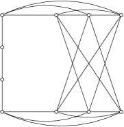
Figure 5.4: A path-cobipartite graph

Figure 5.5: A path-double split graph

Figure 5.6: A graph that has a homogeneous 2-join $(\{a_{1},a_{2}\},$ $\{b_{1},b_{2}\},$ $\{c\},\{d\},$ $\{e_{1},e_{2}\},$ $\{f_{1},f_{2},$ $f_{3},f_{4}\})$

Theorem 5.10 generalizes Theorems 5.2, 5.3 and 5.4: path-cobipartite graphs may be seen either as graphs having a proper path 2-join (Theorems 5.2 and 5.3) or as a new basic class (Theorem 5.4). Path-double split graphs may be seen as graphs having a proper path 2-join (Theorems 5.2 and 5.3) or as graphs having a non-balanced skew partition (Theorem 5.4). And graphs having a homogeneous 2-join may be seen as graphs having a homogeneous pair (Theorems 5.4 and perhaps 5.2) or as graphs having a proper path 2-join (Theorems 5.3 and perhaps 5.2). Formally all these remarks are not always true: it may happen in special cases that path-cobipartite graphs and path-double split graphs have no proper 2-join because the “proper” condition fails. But such graphs are easily established to be basic or to have a balanced skew partition.

Note also that our new basic classes and decomposition yield counter-examples to reckless extensions of Theorems 5.3 and 5.4. The three graphs represented in Fig. 5.4, 5.5, 5.6 are counter-examples to our original conjecture, that is the extension of Theorem 5.3 where path 2-joins are not allowed. Path-double split graphs yield counter-examples to Theorem 5.4 with “balanced skew partition” instead of “skew partition” (see Fig. 5.5). Graphs with a homogeneous 2-join yield counter-examples to Theorem 5.4 where homogeneous pairs are not allowed (see Fig. 5.6). This shows that Theorems 5.3, 5.4 are in a sense best possible, and that to improve them, we need to do what we have done: add more basic classes and decomposition. The three graphs represented in Fig. 5.4, 5.5, 5.6 also show that path cobipartite graphs, path-double split graphs and homogeneous 2-join must somehow appear in our theorem, that is also in a sense best possible.

This work suggests an algorithm for BSP with no reference to a new decomposition theorem. Indeed, the graph $G^{\prime}$ represented in Fig. 5.2 (resp. in Fig. 5.3) is a good candidate to serve as a block of a cutting 2-joins of type 1 (resp. of type 2). The fact that $G^{\prime}$ is bigger than $G$ is not really a problem, since the number of path 2-joins in a graph can be an ingredient of a good notion of size. So, an algorithm might try to deal with path 2-joins by constructing the appropriate block when the 2-join is recognized to be cutting. In fact this was our original idea but it fails: we are not able to recognize cutting 2-joins of type 2. To do this, we would have to guess somehow the sets $A_{3},B_{3}$. But this seems to be exactly the problem of detecting balanced skew partitions, so we are sent back to our original question. Perhaps an astute recursive call to the algorithm would finally bypass this difficulty, at the possible expense of a worse running time. Anyway, we prefer to proceed as we have done, since a new decomposition for Berge graphs is valuable in itself.

Theorem 5.9 gives a structural description of Berge graphs that have no balanced skew partitions: these graphs can be decomposed along 2-joins (and complements of 2-join) till reaching basic graphs. This could be used to solve algorithmic problems for the class of Berge graphs with no balanced skew partitions (together with the Berge graphs recognition algorithm [13], our work solves the recognition in $O(n^{9})$). This class has an unusual feature in the field of perfect graphs: it is not closed under taking induced subgraphs. Theorem 5.9 also gives a structural information on every Berge graph: it can be decomposed in a first step by using only balanced skew partitions, and in a second step by using only 2-joins, possibly in the complement.

A strange feature of the algorithm is that it does not work for general skew partitions in Berge graphs. Because as explained above, we are not able to prove Theorem 5.9 with “skew partition” instead of “balanced skew partition”. Rather than a failure, we consider this as a further indication that balanced skew partition is a relevant decomposition for Berge graphs.

5.4 Decomposing Berge graphs with no skew partitions and no homogeneous pairs

Theorem 5.10 could be used to devise optimization algorithms for Berge graphs with no balanced skew partitions. But these graphs may have homogeneous 2-joins; recall that they are a mixture of path 2-joins and homogeneous pairs, both decompositions that we do not know how to handle. Note that the graph represented in Figure 5.6 is uniquely decomposable by a path 2-join or a homogeneous pair. The aim of this section is to show that excluding homogeneous pairs gives a class with a very useful structure theorem. So, call ${\cal C}^{\text{\scriptsize\sc Berge}}_{\text{\scriptsize\sc no cutset}}$ the class of Berge graphs with no balanced skew partition and no homogeneous pair.

The following theorem is an obvious corollary of Theorem 5.10. This theorem uses non-path 2-joins and, thanks to them, allow to solve the four classical optimization problems: maximum clique, maximum stable set, coloring and coloring of the complement. Note that using 2-joins for optimization seems to be something new, despite folklore rumors saying that it should be possible. The sequel shows that to use 2-joins, many technicalities have to be dealt with.

Call ${\cal C}^{\text{\scriptsize\sc Berge}}_{\text{\scriptsize\sc basic}}$ the class of bipartite, line-graphs of bipartite, path-cobipartite, path-double split graphs and the complements of all these graphs.

Theorem 5.11

If $G$ is in ${\cal C}^{\text{\scriptsize\sc Berge}}_{\text{\scriptsize\sc no cutset}}$, then either $G$ is in ${\cal C}^{\text{\scriptsize\sc Berge}}_{\text{\scriptsize\sc basic}}$ or one of $G,\overline{G}$ has a proper non-path 2-join.

Let ${\cal C}^{\text{\scriptsize\sc parity}}_{\text{\scriptsize\sc}}$ the class of these graphs such that all holes have same parity. We need to define the blocks of decomposition with respect to a 2-join. They are built by replacing each side of the 2-join by a path and the lemma below shows that for graphs in ${\cal C}^{\text{\scriptsize\sc parity}}_{\text{\scriptsize\sc}}$ there exists a unique way to choose the parity of that path.

Lemma 5.12

Let $G$ be a graph in ${\cal C}^{\text{\scriptsize\sc parity}}_{\text{\scriptsize\sc}}$ and $(X_{1},X_{2},A_{1},B_{1},A_{2},B_{2})$ be a split of a proper 2-join of $G$. Then for $i=1,2$, all the paths with an end in $A_{i}$, an end in $B_{i}$ and interior in $C_{i}$ have the same parity.

Let $G$ be a graph and $(X_{1},X_{2},A_{1},B_{1},A_{2},B_{2})$ be a split of a proper 2-join of $G$. Let $k_{1},k_{2}\geq 1$ be integers. The blocks of decomposition of $G$ with respect to $(X_{1},X_{2})$ are the two graphs $G^{k_{1}}_{1},G^{k_{2}}_{2}$ that we describe now. We obtain $G^{k_{1}}_{1}$ by replacing $X_{2}$ by a marker path $P_{2}$, of length $k_{1}$, from a vertex $a_{2}$ complete to $A_{1}$, to a vertex $b_{2}$ complete to $B_{1}$ (the interior of $P_{2}$ has no neighbor in $X_{1}$). The block $G_{2}^{k_{2}}$ is obtained similarly by replacing $X_{1}$ by a marker path $P_{1}$ of length $k_{2}$. We say that $G^{k_{1}}_{1}$ and $G^{k_{2}}_{2}$ are parity-preserving if $G$ is in ${\cal C}^{\text{\scriptsize\sc parity}}_{\text{\scriptsize\sc}}$, for $i=1,2$ and for a path $Q_{i}$ from $A_{i}$ to $B_{i}$ whose intermediate vertices are in $C_{i}$ (and such a path exists since $(X_{1},X_{2})$ is connected), the marker path $P_{i}$ has the same parity as $Q_{i}$. Note that by Lemma 5.12, our definition does not depend on the choice of a particular $Q_{i}$.

The following lemma shows that when decomposing a graph in ${\cal C}^{\text{\scriptsize\sc Berge}}_{\text{\scriptsize\sc no cutset}}$, a unique complementation is possibly needed at the beginning of the process.

Lemma 5.13 (with Vušković [106])

Let $G\in{\cal C}^{\text{\scriptsize\sc Berge}}_{\text{\scriptsize\sc no cutset}}$ and let $(X_{1},X_{2})$ be a proper non-path 2-join of $G$. Let $G^{k_{1}}_{1}$ and $G^{k_{2}}_{2}$ be parity-preserving blocks of decomposition of $G$ w.r.t. $(X_{1},X_{2})$ where $3\leq k_{1},k_{2}\leq 4$. Then $G^{k_{1}}_{1}$ and $G^{k_{2}}_{2}$ are in ${\cal C}^{\text{\scriptsize\sc Berge}}_{\text{\scriptsize\sc no cutset}}$. Moreover, $\overline{G^{k_{1}}_{1}}$ and $\overline{G^{k_{2}}_{2}}$ have no proper 2-join.

But we need more. Indeed, when trying to solve an optimization problem with 2-joins, the idea is to build the 2 blocks and to ask questions recursively to the blocks. Usually, for at least one block, two questions have to be asked (see for instance how we handle maximum cliques in the next section). So, even with a linear number of steps, the number of questions to ask becomes exponential. A classical idea to bypass this problem is the notion of extreme 2-join.

We say that $(X_{1},X_{2})$ is an extreme 2-join if for some $i\in\{1,2\}$ and all $k\geq 3$ the block of decomposition $G_{i}^{k}$ has no proper non-path 2-join. We say that $X_{i}$ is an extreme side of such a 2-join. Figure 5.4 shows that graphs in general do not have an extreme 2-join, but as we now show, graphs with no star cutset do. Having a star-cutset implies having a balanced skew partition (there are a few trivial exceptions: graphs with no edges and graphs on less than 5 vertices). This was noticed by Zambelli [109], a proof can be found in [104]. So, what follows applies to ${\cal C}^{\text{\scriptsize\sc Berge}}_{\text{\scriptsize\sc no cutset}}$ since graphs from this class have no star cutste.

Figure 5.7: Graph $G$ that has a star cutset, but does not have an extreme proper non-path 2-join. $G$ has a proper non-path 2-join represented with bold lines, and all proper non-path 2-joins are equivalent to this one. Both of the blocks of decomposition are isomorphic to graph $H$, and $H$ has a proper non-path 2-join whose edges are represented with bold lines.