Using ILP/SAT to determine pathwidth, visibility representations, and other grid-based graph drawings

Abstract

We present a simple and versatile formulation of grid-based graph representation problems as an integer linear program (ILP) and a corresponding SAT instance. In a grid-based representation vertices and edges correspond to axis-parallel boxes on an underlying integer grid; boxes can be further constrained in their shapes and interactions by additional problem-specific constraints. We describe a general $d$-dimensional model for grid representation problems. This model can be used to solve a variety of NP-hard graph problems, including pathwidth, bandwidth, optimum $st$-orientation, area-minimal (bar-$k$) visibility representation, boxicity-$k$ graphs and others. We implemented SAT-models for all of the above problems and evaluated them on the Rome graphs collection. The experiments show that our model successfully solves NP-hard problems within few minutes on small to medium-size Rome graphs.

1 Introduction

Integer linear programming (ILP) and Boolean satisfiability testing (SAT) are indispensable and widely used tools in solving many hard combinatorial optimization and decision problems in practical applications [2, 8]. In graph drawing, especially for planar graphs, these methods are not frequently applied. A few notable exceptions are crossing minimization [9, 7, 21, 18], orthogonal graph drawing with vertex and edge labels [3] and metro-map layout [25]. Recent work by Chimani et al. [10] uses SAT formulations for testing upward planarity. All these approaches have in common that they exploit problem-specific properties to derive small and efficiently solvable models, but they do not generalize to larger classes of problems.

In this paper we propose a generic ILP model that is flexible enough to capture a large variety of different grid-based graph layout problems, both polynomially-solvable and NP-complete. We demonstrate this broad applicability by adapting the base model to six different NP-complete example problems: pathwidth, bandwidth, optimum $st$-orientation, minimum area bar- and bar $k$-visibility representation, and boxicity-$k$ testing. For minimum-area visibility representations and boxicity this is, to the best of our knowledge, the first implementation of an exact solution method. Of course this flexibility comes at the cost of losing some of the efficiency of more specific approaches. Our goal, however, is not to achieve maximal performance for a specific problem, but to provide an easy-to-adapt solution method for a larger class of problems, which allows quick and simple prototyping for instances that are not too large. Our ILP models can be easily translated into equivalent SAT formulations, which exhibit better performance in the implementation than the ILP models themselves. We illustrate the usefulness of our approach by an experimental evaluation that applies our generic model to the above six NP-complete problems using the well-known Rome graphs [1] as a benchmark set. Our evaluation shows that, depending on the problem, our model can solve small to medium-size instances (sizes varying from about 25 vertices and edges for bar-$1$ visibility testing up to more than 250 vertices and edges, i.e., all Rome graphs, for optimum $st$-orientation) to optimality within a few minutes. In Section 2 we introduce generic grid-based graph representations and formulate an ILP model for $d$-dimensional integer grids. We demonstrate how this model can be adapted to six concrete one-, two- and $d$-dimensional grid-based graph layout problems in Sections 3 and 4. In Section 5 we evaluate our implementations and report experimental results. The implementation is available from i11www.iti.kit.edu/gdsat.

2 Generic Model for Grid-Based Graph Representations

In this section we explain how to express $d$-dimensional boxes in a $d$-dimensional integer grid as constraints of an ILP or a SAT instance. In the subsequent sections we use these boxes as basic elements for representing vertices and edges in problem-specific ILP and SAT models. We need a simple observation that shows that we can restrict ourselves to boxes in integer grids.

Lemma 1

Any set $I$ of $n$ boxes in $\mathbb{R}^{d}$ can be transformed into another set $I^{\prime}$ of $n$ closed boxes on the integer grid $\{1,\ldots,n\}^{d}$ such that two boxes intersect in $I$ if and only if they intersect in $I^{\prime}$.

Proof

Let $I_{1},\dots,I_{n}$ be a set of $d$-dimensional intervals. Then we prove that there exists a set $I^{\prime}_{1},\dots,I^{\prime}_{n}$ of $d$-dimensional intervals such that:

• For all $i$, $I^{\prime}_{i}=[b_{i}^{1},e_{i}^{1}]\times\dots\times[b_{i}^{d},e_{i}^{d}]$ for some $b_{i}^{1},e_{i}^{1},\dots,b_{i}^{d},e_{i}^{d}\in\{1,\dots,n\}$. Put differently, $I^{\prime}_{i}$ has integral coordinates in the range $\{1,\dots,n\}$, and it is closed at both ends.

• $I_{i}\cap I_{j}$ if and only if $I^{\prime}_{i}\cap I^{\prime}_{j}$.

It suffices to show this for 1-dimensional intervals; we can then transform each dimension of the intervals separately to achieve the results for arbitrary dimensions.

For 1-dimensional intervals, presume that $I_{i}=\{s_{i},t_{i}\}$, where we make no assumption over whether the ends of $I_{i}$ are open or closed. We first create a sorted orientation of the $2n$ endpoints of these intervals. We sort them by their coordinate, and in case of a tie take first right endpoints where the interval is open, then left endpoints where the interval is closed, then right endpoints where the interval is closed and then left endpoints where the interval is open. Presume that $\sigma$ describes this order, i.e., for any endpoint $p$ $\sigma(p)$ gives the index of $p$ in this sorted order. One easily verifies that $\{\sigma(s_{i}),\sigma(t_{i})\}$ intersects $\{\sigma(s_{j}),\sigma(t_{j})\}$ if and only if $I_{i}$ intersects $I_{j}$. Here it does not even matter whether we make the new intervals open or closed, since all endpoints are distinct integers.

Now compact $\sigma$ by not using a new integer whenever we have an endpoint of an interval. More precisely, split $\sigma$ into maximal subsequences such that each subsequence consists of multiple (possibly none) left endpoints of intervals, followed by one right endpoint of an interval. There are $n$ such subsequences, since there are $n$ right endpoints. Enumerate the subsequences in order, and let $\sigma^{\prime}(p)$ be the number assigned to the subsequence that contains $\sigma(p)$, for any endpoint $p$ of an interval. Now for $I_{i}=\{s_{i},t_{i}\}$ define $I^{\prime}_{i}$ to be $\left[\sigma^{\prime}(s_{i}),\sigma^{\prime}(t_{i})\right]$. We claim that this satisfies the conditions. Clearly the endpoints of the intervals are integers in the range $1,\dots,n$, so we only must argue that intersections are unchanged. This held when going over from $\{s_{i},t_{i}\}$ to $\{\sigma(s_{i}),\sigma(t_{i})\}$. But going over from $\sigma$ to $\sigma^{\prime}$, we changed the relative order of endpoints only by contracting a number of left endpoints, followed by one right endpoint. Since $I^{\prime}_{i}$ is closed at both ends, this does not change intersections. ∎

2.1 Integer Linear Programming Model

We will describe our model in the general case for a $d$-dimensional integer grid, where $d\geq 1$. Let $\mathcal{R}^{d}=[1,U_{1}]\times\ldots\times[1,U_{d}]$ be a bounded $d$-dimensional integer grid, where $[A,B]$ denotes the set of integers $\{A,A+1,\dots,B-1,B\}$. In a grid-based graph representation vertices and/or edges are represented as $d$-dimensional boxes in $\mathcal{R}^{d}$. A grid box $R$ in $\mathcal{R}^{d}$ is a subset $[s_{1},t_{1}]\times\ldots\times[s_{d},t_{d}]$ of $\mathcal{R}^{d}$, where $1\leq s_{k}\leq t_{k}\leq U_{k}$ for all $1\leq k\leq d$. In the following we describe a set of ILP constraints that together create a non-empty box for some object $v$. We denote this ILP as $\mathcal{B}(d)$.

We first extend $\mathcal{R}^{d}$ by a margin of dummy points to $\bar{\mathcal{R}}^{d}=[0,U_{1}+1]\times\ldots\times[0,U_{d}+1]$. We use three sets of binary variables:

$$x_{\mathbf{i}}(v) \in\{0,1\} \forall\mathbf{i}\in\bar{\mathcal{R}}^{d}$$ (1)

$$b_{i}^{k}(v) \in\{0,1\} \forall 1\leq k\leq d\text{ and }1\leq i\leq U_{k}$$ (2)

$$e_{i}^{k}(v) \in\{0,1\} \forall 1\leq k\leq d\text{ and }1\leq i\leq U_{k}$$ (3)

The variables $x_{\mathbf{i}}(v)$ indicate whether grid point $\mathbf{i}$ belongs to the box representing $v$ ($x_{\mathbf{i}}(v)=1$) or not ($x_{\mathbf{i}}(v)=0$). Variables $b_{i}^{k}(v)$ and $e_{i}^{k}(v)$ indicate whether the box of $v$ may start or end at position $i$ in dimension $k$. We use $\mathbf{i}[k]$ to denote the $k$-th coordinate of grid point $\mathbf{i}\in\mathcal{R}^{d}$ and $\mathbf{1_{k}}=(0,\dots,0,1,0,\dots,0)$ to denote the $k$-th $d$-dimensional unit vector. If $d=1$ we will drop the dimension index of the variables to simplify the notation. The following constraints model a box in $\mathcal{R}^{d}$ (see Fig. 1 for an example):

$$x_{\mathbf{i}}(v) =0 \forall\mathbf{i}\in\bar{\mathcal{R}}^{d}\setminus\mathcal{R}^{d}$$ (4)

$$\sum_{\mathbf{i}\in\bar{\mathcal{R}}^{d}}x_{\mathbf{i}}(v) \geq 1$$ (5)

$$\sum_{{i\in[1,U_{k}]}}b_{i}^{k}(v) =1 \forall 1\leq k\leq d$$ (6)

$$\sum_{{i\in[1,U_{k}]}}e_{i}^{k}(v) =1 \forall 1\leq k\leq d$$ (7)

$$x_{\mathbf{i-1_{k}}}(v)+b_{\mathbf{i}[k]}^{k}(v) \geq x_{\mathbf{i}}(v) \forall\mathbf{i}\in\mathcal{R}^{d}\text{ and }1\leq k\leq d$$ (8)

$$x_{\mathbf{i}}(v) \leq x_{\mathbf{i+1_{k}}}(v)+e_{\mathbf{i}[k]}^{k}(v) \forall\mathbf{i}\in\mathcal{R}^{d}\text{ and }1\leq k\leq d$$ (9)

Constraint (4) creates a margin of zeroes around $\mathcal{R}^{d}$. Constraint (5) ensures that the shape representing $v$ is non-empty, and constraints (6) and (7) provide exactly one start and end position in each dimension. Finally, due to constraints (8) and (9) each grid point inside the specified bounds belongs to $v$ and all other points don’t.

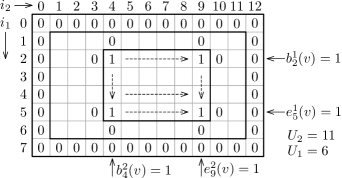
Figure 1: Example of a 2-dimensional $8\times 13$ grid $\bar{\mathcal{R}}^{d}$ with a $6\times 4$ grid box and the corresponding variable assignments.

Lemma 2

The ILP $\mathcal{B}(d)$ defined by constraints (1)–(9) correctly models all non-empty grid boxes in $\mathcal{R}^{d}$.

Proof

Let $R=[s_{1},t_{1}]\times\ldots\times[s_{d},t_{d}]$ be a non-empty grid box in $\mathcal{R}^{d}$. We initially set all variables to the default value of zero. For every $\mathbf{i}\in R$ we set $x_{\mathbf{i}}(R)=1$. Moreover, we set $b_{s_{k}}^{k}(R)=1$ and $e_{t_{k}}^{k}(R)=1$ for all $1\leq k\leq d$. We claim that this assignment satisfies all constraints. Constraints (1)–(3) are obviously satisfied, as well as constraints (4) and (5) since $R$ is nonempty but does not intersect the margin $\bar{\mathcal{R}}^{d}\setminus\mathcal{R}^{d}$. For every $1\leq k\leq d$ we set exactly one variable $b_{i}^{k}(R)=1$ and $e_{j}^{k}(R)=1$, namely for $i=s_{k}$ and $j=t_{k}$; this satisfies constraints (6) and (7). Constraints (8) and (9) are trivially satisfied if $x_{\mathbf{i}}(R)=x_{\mathbf{i+1_{k}}}(R)$ for two neighboring grid points in dimension $k$. Otherwise, if $x_{\mathbf{i-1_{k}}}(R)=0$ and $x_{\mathbf{i}}(R)=1$, then $b_{\mathbf{i}[k]}^{k}$ must equal $1$, and if $x_{\mathbf{i}}(R)=1$ and $x_{\mathbf{i+1_{k}}}(R)=0$, then $e_{\mathbf{i}[k]}^{k}$ must equal $1$. Let $W_{\mathbf{i}}^{k}=\{\mathbf{j}\in\bar{\mathcal{R}^{d}}\mid\mathbf{j}=\mathbf{i}+(\lambda-\mathbf{i}[k])\cdot\mathbf{1_{k}},\,0\leq\lambda\leq U_{k}+1\}$ be a row of $\mathcal{R}^{d}$ in the $k$-th dimension indexed by a grid point $\mathbf{i}$. By $W_{\mathbf{i}}^{k}[l]$ we denote the $l$-th point $\mathbf{i}+(l-\mathbf{i}[k])\cdot\mathbf{1_{k}}$ in row $W_{\mathbf{i}}^{k}$. We know that $x_{\mathbf{j}}(R)=0$ for $\mathbf{j}\in\{W_{\mathbf{i}}^{k}[0],W_{\mathbf{i}}^{k}[U_{k}+1]\}$. If $W_{\mathbf{i}}^{k}\cap R=\emptyset$, then all indicator variables for $W_{\mathbf{i}}^{k}$ are equal to zero and constraints (8) and (9) are satisfied. Otherwise, the indicator variables for row $W_{\mathbf{i}}^{k}$ contain a consecutive sequence of $1$’s for points $W_{\mathbf{i}}^{k}[l]\in R$ with $s_{k}\leq l\leq t_{k}$. But since $b_{s_{k}}^{k}(R)=1$ and $e_{t_{k}}^{k}(R)=1$ the constraints (8) and (9) are also satisfied for $\mathbf{j}=W_{\mathbf{i}}^{k}[s_{k}]$ and $\mathbf{j}=W_{\mathbf{i}}^{k}[t_{k}]$.

Now consider a valid variable assignment according to constraints (1)–(9) and define $R=\{\mathbf{i}\in\mathcal{R}^{d}\mid x_{\mathbf{i}}=1\}$. By constraints (4) and (5) $R$ contains at least one point. Let $1\leq k\leq d$ be a dimension of $\mathcal{R}^{d}$ and let $W_{\mathbf{i}}^{k}$ be any row in the $k$-th dimension. By constraints (6) and (7) there is exactly one coordinate $s_{k}$, where $b_{s_{k}}^{k}=1$ and one coordinate $t_{k}$, where $e_{t_{k}}^{k}=1$. Thus by constraints (8) and (9) $W_{\mathbf{i}}^{k}\cap R$ is either empty or a single interval of consecutive points between $W_{\mathbf{i}}^{k}[s_{k}]$ and $W_{\mathbf{i}}^{k}[t_{k}]$. Since this is true for any $k$, the set $R$ must be a (non-empty) grid box. ∎

Our example ILP models in Sections 3 and 4 extend ILP $\mathcal{B}(d)$ by additional constraints controlling additional properties of vertex and edge boxes. For instance, boxes can be easily constrained to be single points, to be horizontal or vertical line segments, to intersect if and only if they are incident or adjacent in $G$, to meet in endpoints etc. The definition of an objective function for the ILP depends on the specific problem at hand and will be discussed in the problem sections.

2.2 Translating the ILP model into a SAT model

In this section we explain shortly how ILP $\mathcal{B}(d)$ can be translated into an equivalent SAT formulation with better practical performance. The transformation of $\mathcal{B}(d)$ (including later problem-specific extensions) into a SAT instance, i.e., a set of Boolean clauses, is straightforward. Let $k,c\in\mathbb{N}\setminus\{0\}$, $k>c$, be positive integers and $y_{1},\ldots,y_{k}$, $z$ be binary variables. Then most of our ILP constraints belong to one of the following four types: (i) $\sum_{i=1}^{k}y_{i}\geq z$, (ii) $\sum_{i=1}^{k}y_{i}\leq c$, (iii) $\sum_{i=1}^{k}y_{i}\geq c$, (iv) $\sum_{i=1}^{k}y_{i}=c$.

We translate a type-(i) constraint into the clause $y_{1}\vee\ldots\vee y_{k}\vee\neg z$. For a type-(ii) constraint we consider each tuple of $c+1$ pairwise distinct indices $i_{1},\ldots,i_{c+1}$ and add the clause $\neg y_{i_{1}}\vee\ldots\vee\neg y_{i_{c}}\vee\neg y_{i_{c+1}}$. This gives us $\binom{k}{c+1}$ clauses of size $c+1$. A type-(iii) constraint is equivalent to $\sum_{i=1}^{k}(1-y_{i})\leq k-c$, providing $\binom{k}{k-c+1}$ clauses of size $k-c+1$. A type-(iv) constraint is described as a type-(ii) and a type-(iii) constraint and thus needs $\binom{k}{c+1}$ clauses of size $c+1$ and $\binom{k}{k-c+1}$ clauses of size $k-c+1$.

3 One-dimensional Problems

In the following, let $G=(V,E)$ be an undirected graph with $|V|=n$ and $|E|=m$. One-dimensional grid-based graph representations can be used to model vertices as intersecting intervals (one-dimensional boxes) or as disjoint points that induce a certain vertex order. We present ILP models for three such problems.

3.1 Pathwidth

The pathwidth of a graph $G$ is a well-known graph parameter with many equivalent definitions. We use the definition via the smallest clique size of an interval supergraph. More precisely, a graph is an interval graph if it can be represented as intersection graph of 1-dimensional intervals. A graph $G$ has pathwidth $pw(G)\leq p$ if there exists an interval graph $H$ that contains $G$ as a subgraph and for which all cliques have size at most $p+1$. It is NP-hard to compute the pathwidth of an arbitrary graph and even hard to approximate it [4]. There are fixed-parameter algorithms for computing the pathwidth, e.g. [5], however, we are not aware of any implementations of these algorithms. The only available implementations are exponential-time algorithms, e.g., in sage.

Problem 1 (Pathwidth)

Given a graph $G=(V,E)$, determine the pathwidth of $G$, i.e., the smallest integer $p$ so that $pw(G)\leq p$.

There is an interesting connection between pathwidth and planar graph drawings of small height. Any planar graph that has a planar drawing of height $h$ has pathwidth at most $h$ [17]. Also, pathwidth is a crucial ingredient in testing in polynomial time whether a graph has a planar drawing of height $h$ [14].

We create a one-dimensional grid representation of $G$, in which every vertex is an interval and every edge forces the two vertex intervals to intersect. The objective is to minimize the maximum number of intervals that intersect in any given point. We use the ILP $\mathcal{B}(1)$ for a grid $\mathcal{R}=[1,n]$, which already assigns a non-empty interval to each vertex $v\in V$. We add binary variables for the edges of $G$, a variable $p\in\mathbb{N}$ representing the pathwidth of $G$, and a set of additional constraints as follows.

$$x_{i}(e) \in\{0,1\} \forall{i}\in{\mathcal{R}}\text{ and }e\in E$$ (10)

$$\sum_{i\in\mathcal{R}}x_{i}(e) \geq 1 \forall e\in E$$ (11)

$$x_{i}(uv) \leq x_{i}(u), x_{i}(uv) \leq x_{i}(v) \forall uv\in E$$ (12)

$$\sum_{v\in V}x_{i}(v) \leq p+1 \forall i\in\mathcal{R}$$ (13)

Our objective function is to minimize the value of $p$ subject to the above constraints.

It is easy to see that every edge must be represented by some grid point (constraint (11)), and can only use those grid points, where the two end vertices intersect (constraint (12)). Hence the intervals of vertices define some interval graph $H$ that is a supergraph of $G$. Constraint (13) enforces that at most $p+1$ intervals meet in any point, which by Helly’s property means that $H$ has clique-size at most $p+1$. So $G$ has pathwidth at most $p$. By minimizing $p$ we obtain the desired result. In our implementation we translate the ILP into a SAT instance using the rules given in Section 2.2. We test satisfiability for fixed values of $p$, starting with $p=1$ and increasing it incrementally until a solution is found.

Theorem 3.1

There exists an ILP/SAT formulation with $O(n(n+m))$ variables and $O(n(n+m))$ constraints / $O(n^{3}+n\binom{n}{p+2})$ clauses of maximum size $n$ that has a solution of value $\leq p$ if and only if $G$ has pathwidth $\leq p$.

With some easy modifications, the above ILP can be used for testing whether a graph is a (proper) interval graph. Section 4.2 shows that boxicity-$d$ graphs, the $d$-dimensional generalization of interval graphs, can also be recognized by our ILP.

3.2 Bandwidth

The bandwidth of a graph $G$ with $n$ vertices is another classic graph parameter, which is NP-hard to compute [11]; due to the practical importance of the problem there are also a few approaches to find exact solutions to the bandwidth minimization problem. For example, [13] and [24] use the branch-and-bound technique combined with various heuristics. We present a solution that can be easily described using our general framework. However, regarding the running time, it cannot be expected to compete with techniques specially tuned for solving the bandwidth minimization problem.

Let $f:V\rightarrow\{1,\dots,n\}$ be a bijection that defines a linear vertex order. The bandwidth of $G$ is defined as $bw(G)=\min_{f}\max\{f(v)-f(u)\mid uv\in E\text{ and }f(u)<f(v)\}$, i.e., the minimum length of the longest edge in $G$ over all possible vertex orders.

We describe an ILP that assigns the vertices of $G$ to disjoint grid points and requires for an integer $k$ that any pair of adjacent vertices is at most $k$ grid points apart. If the ILP has a solution, then we know $bw(G)\leq k$. We set $\mathcal{R}=[1,n]$ and add the following two constraints:

$$\sum_{v\in V}x_{i}(v) \leq 1 \forall i\in\mathcal{R}$$ (14)

$$x_{i}(u) \leq\sum_{j=i-k}^{i+k}x_{j}(v) \forall uv\in E\,\forall i\in\mathcal{R}$$ (15)

Constraint (14) guarantees that no grid point is occupied by more than one vertex, and constraint (15) requires that any two adjacent vertices are at most $k$ grid points apart. We note that the variables $b_{i}(v)$ and $e_{i}(v)$ and their constraints are not required in this model since in $\mathcal{R}=[1,n]$ constraints (5) and (14) suffice to set exactly one variable $x_{i}(v)=1$ for every $v\in V$. We do not need an objective function but rather test if the feasible region is non-empty for a given $k\geq 1$.

Theorem 3.2

There exists an ILP/SAT formulation with $O(n^{2})$ variables and $O(n\cdot m)$ constraints / $O(n^{3})$ clauses of maximum size $n$ that has a solution if and only if $G$ has bandwidth $\leq k$.

3.3 Optimum $st$-orientation

Let $G$ be an undirected graph and let $s$ and $t$ be two vertices of $G$ with $st\in E$. An $st$-orientation of $G$ is an orientation of the edges such that $s$ is the unique source and $t$ is the unique sink [16]. Such an orientation can exist only if $G$ is biconnected. Computing an $st$-orientation can be done in linear time [16, 6], but it is NP-complete to find an $st$-orientation that minimizes the length of the longest path from $s$ to $t$, even for planar graphs [27]. It has many applications in graph drawing [26] and beyond.

Problem 2 (Optimum $st$-orientation)

Given a graph $G=(V,E)$ and two vertices $s,t\in V$ with $st\in E$, find an orientation of $E$ such that $s$ is the only source, $t$ is the only sink, and the length of the longest directed path from $s$ to $t$ is minimum.

We now formulate an ILP that computes a height-$k$ $st$-orientation of $G$, i.e., an $st$-orientation such that the longest path has length at most $k$ (if one exists). We use the ILP $\mathcal{B}(1)$ for $\mathcal{R}=[1,k]$ to assign intervals to the vertices and edges of $G$. Vertices are required to occupy exactly one point, whereas edges must span at least two points. The additional constraints are as follows:

$$\sum_{i\in\mathcal{R}}x_{i}(v) \leq 1 \forall v\in V$$ (16)

$$\sum_{i\in\mathcal{R}}x_{i}(e) \geq 2 \forall e\in E$$ (17)

$$b_{i}(uv) \leq x_{i}(u)+x_{i}(v), e_{i}(uv) \leq x_{i}(u)+x_{i}(v) \forall i\in\mathcal{R}\,\forall uv\in E$$ (18)

$$x_{i}(v) \leq\sum_{vw\in E}b_{i}(vw) \forall i\in\mathcal{R}\,\forall v\in V\setminus\{t\}$$ (19)

$$x_{i}(v) \leq\sum_{vw\in E}e_{i}(vw) \forall i\in\mathcal{R}\,\forall v\in V\setminus\{s\}$$ (20)

Similarly to the ILP in Section 3.2, the variables $b_{i}(v)$ and $e_{i}(v)$ and their constraints are not required for the vertices, since constraints (5) and (16) ensure that every vertex interval consists of a single grid point. Constraint (17) guarantees that each edge interval contains at least two points. Constraint (18) makes sure that every edge must begin and end at the grid points occupied by its end vertices. Finally, constraints (19) and (20) ensure that every vertex except $t$ has an outgoing edge and every vertex except $s$ has an incoming edge. Since $\mathcal{R}=[1,k]$ and adjacent vertices cannot occupy the same grid point, we know that if this ILP has a feasible solution, then the longest directed path from $s$ to $t$ has length at most $k$. Alternatively, we can set $k=n$ and use the objective function $\min\sum_{i=1}^{n}i\cdot x_{i}(t)$ to minimize the position of the sink $t$ and thus the longest path from $s$ to $t$.

Theorem 3.3

There exists an ILP with $O(n(n+m))$ variables and constraints that computes an optimum $st$-orientation. Alternatively, there exists an ILP/SAT formulation with $O(k(n+m))$ variables and $O(k(n+m))$ constraints / $O(k^{2}(n+m))$ clauses of maximum size $n$ that has a solution if and only if a height-$k$ $st$-orientation of $G$ exists.

4 Higher-Dimensional Problems

In this section we give examples of two-dimensional visibility graph representations and a $d$-dimensional grid-based graph representation problem. Let again $G=(V,E)$ be an undirected graph with $|V|=n$ and $|E|=m$.

4.1 Visibility representations

A visibility representation (also: bar visibility representation or weak visibility representation) of a graph $G=(V,E)$ maps all vertices to disjoint horizontal line segments, called bars, and all edges to disjoint vertical bars, such that for each edge $uv\in E$ the bar of $uv$ has its endpoints on the bars for $u$ and $v$ and does not intersect any other vertex bar. Visibility representations are an important visualization concept in graph drawing, e.g., it is well known that a graph is planar if and only if it has a visibility representation [29, 28]. An interesting recent extension are bar $k$-visibility representations [12], which additionally allow edges to intersect at most $k$ non-incident vertex bars. We use our ILP to compute compact visibility and bar $k$-visibility representations. Minimizing the area of a visibility representation is NP-hard [23] and we are not aware of any implemented exact algorithms to solve the problem for any $k\geq 0$. By Lemma 1 we know that all bars can be described with integer coordinates of size $O(m+n)$.

Problem 3 (Bar $k$-Visibility Representation)

Given a graph $G$, an integer grid of size $H\times W$, and an integer $k\geq 0$, find a bar $k$-visibility representation on the given grid (if one exists).

Bar visibility representations.

Our goal is to test whether $G$ has a visibility representation in a grid with $H$ columns and $W$ rows (and thus minimize $H$ or $W$). We set $\mathcal{R}^{2}=[1,H]\times[1,W]$ and use ILP $\mathcal{B}(2)$ to create grid boxes for all edges and vertices in $G$. We add one more set of binary variables for vertex-edge incidences and the following constraints.

$$x_{\mathbf{i}}(e,v) \in\{0,1\} \forall\mathbf{i}\in\mathcal{R}^{2}\,\forall e\in E\,\forall v\in e$$ (21)

$$b_{i}^{1}(v) =e_{i}^{1}(v) \forall i\in[1,U_{1}]\,\forall v\in V$$ (22)

$$b_{i}^{2}(e) =e_{i}^{2}(e) \forall i\in[1,U_{2}]\,\forall e\in E$$ (23)

$$\sum_{v\in V}x_{\mathbf{i}}(v) \leq 1 \forall\mathbf{i}\in\mathcal{R}^{2}$$ (24)

$$\sum_{v\in V\setminus e}x_{\mathbf{i}}(v) \leq(1-x_{\mathbf{i}}(e)) \forall\mathbf{i}\in\mathcal{R}^{2}\,\forall e\in E$$ (25)

$$x_{\mathbf{i}}(e,v) \leq x_{\mathbf{i}}(e), x_{\mathbf{i}}(e,v) \leq x_{\mathbf{i}}(v) \forall\mathbf{i}\in\mathcal{R}^{2}\,\forall e\in E\,\forall v\in e$$ (26)

$$\sum_{\mathbf{i}\in\mathcal{R}^{2}}x_{\mathbf{i}}(e,v) \geq 1 \forall e\in E\,\forall v\in e$$ (27)

$$x_{\mathbf{i}}(e,v) \leq b_{\mathbf{i}[1]}^{1}(e)+e_{\mathbf{i}[1]}^{1}(e) \forall\mathbf{i}\in\mathcal{R}^{2}\,\forall e\in E\,\forall v\in e$$ (28)

Constraints (22) and (23) ensure that all vertex boxes are horizontal bars of height 1 and all edge boxes are vertical bars of width 1. Constraint (24) forces the vertex boxes to be disjoint; edge boxes will be implicitly disjoint due to the remaining constraints. No edge is allowed to intersect a non-incident vertex due to constraint (25). Finally, we need to set the new incidence variables $x_{\mathbf{i}}(e,v)$ for an edge $e$ and an incident vertex $v$ so that $x_{\mathbf{i}}(e,v)=1$ if and only if $e$ and $v$ share the grid point $\mathbf{i}$. Constraints (26) and (27) ensure that each incidence in $G$ is realized in at least one grid point, but it must be one that is used by the boxes of $e$ and $v$. Finally, constraint (28) requires edge $e$ to start and end at its two intersection points with the incident vertex boxes. This constraint is optional, but yields a tighter formulation.To transform constraint (25) into SAT, we add the clause $\neg x_{\mathbf{i}}(e)\vee\neg x_{\mathbf{i}}(v)$ for each $\mathbf{i}\in\mathcal{R}^{2}$, $e\in E$, $v\in V\setminus e$, and apply the general transformation rules otherwise.

Since every graph with a visibility representation is planar (and vice versa) we have $m\in O(n)$. Moreover, our ILP and SAT models can also be used to test planarity of a given graph by setting $H=n$ and $W=2n-4$, which is sufficient due to Tamassia and Tollis [28]. This might not look interesting at first sight since planarity testing can be done in linear time [20]. However, we think that this is still useful as one can add other constraints to the ILP model, e.g., to create simultaneous planar embeddings, and use it as a subroutine for ILP formulations of applied graph drawing problems such as metro maps [25] and cartograms.

Theorem 4.1

There exists an ILP/SAT formulation with $O(HWn)$ variables and $O(HWn)$ constraints / $O(HWn^{2})$ clauses of maximum size $HW$ that solves Problem 3 for $k=0$.

Bar $k$-visibility representations.

It is easy to extend our previous model for $k=0$ to test bar $k$-visibility representations for $k\geq 1$. We drop constraint (25), introduce another set of binary variables to indicate intersections between edges and non-incident vertices, and add the following constraints.

$$y_{\mathbf{i}}(e) \in\{0,1\} \forall\mathbf{i}\in\mathcal{R}^{2}\,\forall e\in E$$ (29)

$$x_{\mathbf{i}}(e)+\sum_{v\in V\setminus e}x_{\mathbf{i}}(v) \leq y_{\mathbf{i}}(e)+1 \forall\mathbf{i}\in\mathcal{R}^{2}\,\forall e\in E$$ (30)

$$\sum_{\mathbf{i}\in\mathcal{R}^{2}}y_{\mathbf{i}}(e) \leq k \forall e\in E$$ (31)

$$x_{\mathbf{i}}(e)+x_{\mathbf{i}}(e^{\prime})-\frac{1}{2}(b_{\mathbf{i}[1]}^{1}(e)+e_{\mathbf{i}[1]}^{1}(e)+b_{\mathbf{i}[1]}^{1}(e^{\prime})+e_{\mathbf{i}[1]}^{1}(e^{\prime}))\leq 1\,\forall\mathbf{i}\in\mathcal{R}^{2}\,\forall(e,e^{\prime})\in\binom{E}{2}$$ (32)

The variable $y_{\mathbf{i}}(e)$ is supposed to equal 1 if and only if $e$ intersects a non-incident vertex at position $\mathbf{i}$. Constraint (30) enforces that $y_{\mathbf{i}}(e)=1$ if grid point $\mathbf{i}$ is occupied by $e$ and a non-incident vertex and constraint (31) makes sure that no more than $k$ such non-incident bars are crossed by each edge. Finally, constraint (32) guarantees that any two edge bars are disjoint, except for the case that they are incident to the same vertex bar and meet at a common endpoint. (Alternatively, we could enforce disjointness for all edge bars if we required vertex bars of height $2$.)

To transform constraint (30) into SAT, we add clause $\neg x_{\mathbf{i}}(e)\vee\neg x_{\mathbf{i}}(v)\vee y_{\mathbf{i}}(e)$ for each $\mathbf{i}\in\mathcal{R}^{2}$, $e\in E$, $v\notin e$. For (32), we add $\neg x_{\mathbf{i}}(e)\vee\neg x_{\mathbf{i}}(e^{\prime})\vee b_{\mathbf{i}[1]}^{1}(e)\vee e_{\mathbf{i}[1]}^{1}(e)$ for each ordered pair $e,e^{\prime}\in E$, $e\neq e^{\prime}$. For the rest of the constraints, we apply the general transformation rules.

Theorem 4.2

There exists an ILP/SAT formulation with $O(HW(n+m))$ variables and $O(HW(m^{2}+n))$ constraints / $O(\binom{HW}{k+1}m+HWm^{2})$ clauses of maximum size $HW$ that solves Problem 3 for $k\geq 1$.

4.2 Boxicity-$d$ graphs

A graph is said to have boxicity $d$ if it can be represented as intersection graph of $d$-dimensional axis-aligned boxes. Testing whether a graph has boxicity $d$ is NP-hard, even for $d=2$ [22]. We are not aware of any implemented algorithms to determine the boxicity of a graph. By Lemma 1 we can restrict ourselves to a grid of side length $n$.

We use ILP $\mathcal{B}(d)$ for $\mathcal{R}^{d}=[1,n]^{d}$ to model a $d$-dimensional box for each vertex of a graph $G=(V,E)$. We add the following variables and constraints to achieve the correct intersection properties.

$$x_{\mathbf{i}}(e) \in\{0,1\} \forall\mathbf{i}\in\mathcal{R}^{d}\,\forall e\in E$$ (33)

$$\sum_{\mathbf{i}\in\mathcal{R}^{d}}x_{\mathbf{i}}(e) \geq 1 \forall e\in E$$ (34)

$$x_{\mathbf{i}}(uv) \leq x_{\mathbf{i}}(u), x_{\mathbf{i}}(uv) \leq x_{\mathbf{i}}(v) \forall\mathbf{i}\in\mathcal{R}^{d}\,\forall uv\in E$$ (35)

$$x_{\mathbf{i}}(u)+x_{\mathbf{i}}(v) \leq 1 \forall\mathbf{i}\in\mathcal{R}^{d}\,\forall uv\in\binom{V}{2}\setminus E$$ (36)

The variables $x_{\mathbf{i}}(e)$ indicate whether a grid point lies in the intersection of two boxes and thus represents an edge. Constraint (34) guarantees that there is a non-empty intersection for each edge $e\in E$, and by constraint (35) we make sure that the intersection indicator for an edge $uv$ can only be set to $1$ at position $\mathbf{i}$ if the grid boxes for $u$ and $v$ both occupy point $\mathbf{i}$. Finally, constraint (36) enforces that no grid point can be occupied by a pair of non-adjacent vertices.

Theorem 4.3

There exists an ILP with $O(n^{d}(n+m))$ variables and $O(n^{d+2})$ constraints as well as a SAT instance with $O(n^{d}(n+m))$ variables and $O(n^{d+2})$ clauses of maximum size $O(n^{d})$ to test whether a graph $G$ has boxicity $d$.

5 Experiments

We implemented and tested our formulation for minimizing pathwidth, bandwidth, length of longest path in an $st$-orientation, and width of bar-visibility and bar 1-visibility representations, as well as deciding whether a graph has boxicity 2.

The experiments were performed on a single core of an AMD Opteron 6172 processor running Linux 3.4.11. The machine is clocked at 2.1 Ghz, and has 256 GiB RAM. Our implementation is written in C++ and was compiled with GCC 4.7.1 using optimization -O3. As test sample we used the Rome graphs dataset [1] which consists of 11533 graphs with vertex number between 10 and 100. $18\%$ of the Rome graphs are planar. Figure 2 shows the size distribution of the Rome graphs.

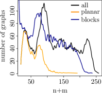
Figure 2: Size distribution of Rome graphs. Black: all graphs, blue: biconnected blocks ($n{\geq}3$), orange: planar graphs. We used an $(1,2,3,2,1)$-Gaussian filter to reduce oscillations.

We initially used the Gurobi solver [19] to test the implementation of the ILP formulations, however it turned out that even for very small graphs ($n<10$) solving a single instance can take minutes. We therefore focused on the equivalent SAT formulations gaining a significant speed-up. As SAT solver we used MiniSat [15] in version 2.2.0. For each of the five minimization problems we determined obvious lower and upper bounds in $O(n)$ for the respective graph parameter. Starting with the lower bound we iteratively increased the parameter to the next integer until a solution was found (or a predefined timeout was exceeded). Each iteration consists of constructing the SAT formulation and executing the SAT solver. We measured the total time spent in all iterations. For boxicity 2 we decided to consider square grids and minimize their side lengths. Thus the same iterative procedure applies to boxicity 2.

Note that for all considered problems a binary search-like procedure for the parameter value did not prove to be efficient, since the solver usually takes more time with increasing parameter value, which is mainly due to the increasing number of variables and clauses. For the one-dimensional problems we used a timeout of 300 seconds, for the two-dimensional problems of 600 seconds.

We ran the instances sorted by size $n+m$ starting with the smallest graphs. If more than 400 consecutive graphs in this order produced timeouts, we ended the experiment prematurely and evaluated only the so far obtained results. Figures 3 and 4 summarize our experimental results and show the percentage of Rome graphs solved within the given time limit, as well as scatter plots with each solved instance represented as a point depending on its graph size and the required computation time.

(a) percentage of solved instances

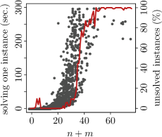
(b) pathwidth

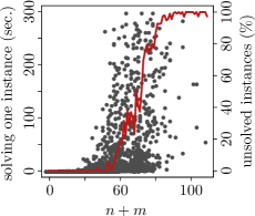
(c) bandwidth

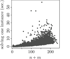
(d) $st$-orientation

Figure 3: Experimental results for the one-dimensional problems. LABEL:sub@fig:solved Percentage of solved instances. LABEL:sub@fig:pw:time–LABEL:sub@fig:st:time: Time in seconds for solving an instance (dots) and percentage of instances not solved within 300 seconds (red curves), both in relation to $n+m$

Pathwidth. As Fig. 3a shows, we were able to compute the pathwidth for $17.0\%$ of all Rome graphs, from which $82\%$ were solved within the first minute and only $3\%$ within the last. Therefore, we expect that a significant increase of the timeout value would be necessary for a noticeable increase of the percentage of solved instances. We note that almost all small graphs ($n+m<45$) could be solved within the given timeout, however, for larger graphs, the percentage of solved instances rapidly drops, as the red curve in Fig. 3b shows. Almost no graphs with $n+m>70$ were solved.

Bandwidth. We were able to compute the bandwidth for $22.3\%$ of all Rome graphs (see Fig. 3a), from which $90\%$ were solved within the first minute and only $1.3\%$ within the last. Similarly to the previous case, the procedure terminated successfully within 300 seconds for almost all small graphs ($n+m<55$ in this case), while almost none of the larger graphs ($n+m>80$) were solved; see the red curve in Fig. 3c.

Optimum $st$-orientation. Note that very few of the Rome graphs are biconnected. Therefore, to test our SAT implementation for computing the minimum number of levels in an $st$-orientation, we subdivided each graph into biconnected blocks and removed those with $n\leq 2$, which produced 13606 blocks in total; see Fig. 2 for the distribution of block sizes. Then, for each such block, we randomly selected one pair of vertices $s,t$, $s\neq t$, connected them by an edge if it did not already exist and ran the iterative procedure. In this way, for the respective choice of $s,t$ we were able to compute the minimum number of levels in an $st$-orientation for all biconnected blocks; see Fig. 3a. Moreover, no graph took longer than 57 seconds, for $97\%$ of the graphs it took less than 10 seconds and for $68\%$ less than 3 seconds. Even for the biggest blocks with $m+n>200$, the procedure successfully terminated within 15 seconds in $93\%$ of the cases; see Fig. 3d.

(a) percentage of solved instances

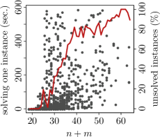
(b) bar visibility

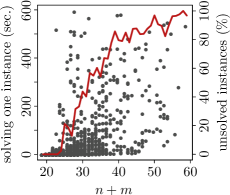
(c) bar 1-visibility

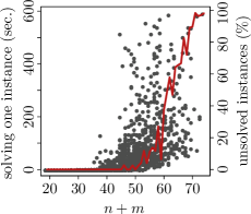
(d) boxicity 2

Figure 4: Experimental results for the two-dimensional problems. LABEL:sub@fig:visrep:solved Percentage of solved instances. The red horizontal line shows the percentage of planar graphs over all Rome graphs. LABEL:sub@fig:visrep:time–LABEL:sub@fig:box:time: Time in seconds for solving an instance (dots) and percentage of instances not solved within 600 seconds (red curves), both in relation to $n+m$.

Bar visibility. To compute bar-visibility representations of minimum width, we iteratively tested for each graph all widths $W$ between 1 and n. We used the trivial upper bound $H=n$ for the height. We were able to compute solutions for $28.5\%$ of all 3281 planar Rome graphs (see Fig. 4a), $69\%$ of which were solved within the first minute and less than $0.1\%$ within the last. We were able to solve all small instances with $n+m\leq 23$ and almost none for $n+m>55$; see the red curve in Fig. 4b.

Bar 1-visibility. We also ran the width minimization procedure for bar 1-visibility representations on all Rome graphs. The number of graphs for which the procedure terminated successfully within the given time is 833 ($7.2\%$ of all Rome graphs), which is close to the corresponding number for bar-visibility; see Fig. 4a. This is not surprising, since most small Rome graphs are planar; see Fig. 2. For bar 1-visibility, eight graphs were solved which were not solved for bar-visibility. Interestingly, they were all planar. All but 113 graphs successfully processed in the previous experiment were also successfully processed in this one. A possible explanation for those 113 graphs is that the SAT formulation for bar 1-visibility requires more clauses. All small graphs with $n+m\leq 23$ were processed successfully. Interestingly, for none of the processed graphs the minimum width actually decreased in comparison to their minimum-width bar-visibility representation.

Boxicity-2 For testing boxicity 2, we started with a $3\times 3$ grid for each graph and then increased height and width simultaneously after each iteration. Within the specified timeout of 600 seconds, we were able to decide whether a graph has boxicity 2 for $18.7\%$ of all Rome graphs (see Fig. 4b), $82\%$ of which were processed within the first minute and $0.3\%$ within the last. All of the successfully processed graphs actually had boxicity 2. Small graphs with $n+m\leq 50$ were processed almost completely, while almost none of the graphs with $n+m>70$ finished; see Fig. 4d.

6 Conclusion

We presented a versatile ILP formulation for determining placement of grid boxes according to problem-specific constraints. We gave six examples of how to extend this formulation for solving numerous NP-hard graph drawing and graph representation problems, such as bar-visibility representations, computing the pathwidth and the boxicity, and finding an st-orientation that minimizes the longest directed path. Our experimental evaluation showed that while solving the original ILP is rather slow, the easily derived SAT formulations perform quite well for smaller graphs. While our approach is not suitable to replace specialized exact or heuristic algorithms that are faster and/or can solve larger instances of these problems, it does provide a simple-to-use tool for solving problems that can be modeled by grid-based graph representations without much implementation effort. This can be useful, e.g., for verifying counterexamples, NP-hardness gadgets, or for computing solutions to certain instances in practice.

We note that many other problems can easily be formulated as ILPs by assigning grid-boxes to vertices or edges. Among those are, e.g., testing whether a planar graph has a straight-line drawing of height $h$, testing whether a planar graph has a rectangular dual with integer coordinates and prescribed integral areas, testing whether a graph is a $t$-interval graph, or whether a bipartite graph can be represented as a planar bus graph. Important open problems are to reduce the complexity of our formulations and the question whether approximation algorithms for graph drawing can be derived from our model via fractional relaxation.

References

- [1] Rome graphs. www.graphdrawing.org/download/rome-graphml.tgz.
- [2] A. Biere, M. Heule, H. van Maaren, and T. Walsh, editors. Handbook of Satisfiability. IOS Press, 2009.
- [3] C. Binucci, W. Didimo, G. Liotta, and M. Nonato. Orthogonal drawings of graphs with vertex and edge labels. Comput. Geom. Theory Appl., 32(2):71–114, 2005.
- [4] H. L. Bodlaender, J. R. Gilbert, T. Kloks, and H. Hafsteinsson. Approximating treewidth, pathwidth, and minimum elimination tree height. In Proc. Workshop Graph-Theoretic Concepts Comput. Sci. (WG’91), volume 570 of LNCS, pages 1–12. Springer, 1992.
- [5] H. L. Bodlaender and T. Kloks. Efficient and constructive algorithms for the pathwidth and treewidth of graphs. J. Algorithms, 21(2):358–402, 1996.
- [6] U. Brandes. Eager ordering. In Europ. Symp. Algorithms (ESA’02), volume 2461 of LNCS, pages 247–256. Springer, 2002.
- [7] C. Buchheim, M. Chimani, D. Ebner, C. Gutwenger, M. Jünger, G. W. Klau, P. Mutzel, and R. Weiskircher. A branch-and-cut approach to the crossing number problem. Discrete Optimization, 5(2):373–388, 2008.
- [8] D.-S. Chen, R. G. Batson, and Y. Dang. Applied Integer Programming. Wiley, 2010.
- [9] M. Chimani, P. Mutzel, and I. Bomze. A new approach to exact crossing minimization. In Europ. Symp. Algorithms (ESA’08), volume 5193 of LNCS, pages 284–296. Springer, 2008.
- [10] M. Chimani and R. Zeranski. Upward planarity testing via SAT. In Graph Drawing 2012, volume 7704 of LNCS, pages 248–259. Springer, 2013.
- [11] P. Z. Chinn, J. Chvátalova, A. K. Dewdney, and N. E. Gibbs. The bandwidth problem for graphs and matrices—a survey. J. Graph Theory, 6(3):223–254, 1982.
- [12] A. M. Dean, W. Evans, E. Gethner, J. D. Laison, M. A. Safari, and W. T. Trotter. Bar -visibility graphs. J. Graph Algorithms Appl., 11(1):45–59, 2007.
- [13] G. M. Del Corso and G. Manzini. Finding exact solutions to the bandwidth minimization problem. Computing, 62(3):189–203, 1999.
- [14] V. Dujmovic, M. R. Fellows, M. Kitching, G. Liotta, C. McCartin, N. Nishimura, P. Ragde, F. A. Rosamond, S. Whitesides, and D. R. Wood. On the parameterized complexity of layered graph drawing. Algorithmica, 52(2):267–292, 2008.
- [15] N. Eén and N. Sörensson. An extensible SAT-solver. In Proc. Theory and Appl. of Satisfiability Testing (SAT’03), volume 2919 of LNCS, pages 502–518. Springer, 2004.
- [16] S. Even and R. E. Tarjan. Computing an st-numbering. Theoret. Comput. Sci., 2(3):339–344, 1976.
- [17] S. Felsner, G. Liotta, and S. Wismath. Straight-line drawings on restricted integer grids in two and three dimensions. J. Graph Algorithms Appl., 7(4):363–398, 2003.
- [18] G. Gange, P. J. Stuckey, and K. Marriott. Optimal k-level planarization and crossing minimization. In Graph Drawing 2010, volume 6502 of LNCS, pages 238–249. Springer, 2011.
- [19] Gurobi Optimization, Inc. Gurobi optimizer reference manual, 2013.
- [20] J. Hopcroft and R. Tarjan. Efficient planarity testing. J. ACM, 21(4):549–568, Oct. 1974.
- [21] M. Jünger and P. Mutzel. 2-layer straightline crossing minimization: Performance of exact and heuristic algorithms. J. Graph Algorithms Appl., 1(1):1–25, 1997.
- [22] J. Kratochvíl. A special planar satisfiability problem and a consequence of its np-completeness. Discrete Appl. Math., 52(3):233–252, Aug. 1994.
- [23] X. Lin and P. Eades. Towards area requirements for drawing hierarchically planar graphs. Theoret. Comput. Sci., 292(3):679–695, 2003.
- [24] R. Martí, V. Campos, and E. Piñana. A branch and bound algorithm for the matrix bandwidth minimization. Europ. J. of Operational Research, 186:513–528, 2008.
- [25] M. Nöllenburg and A. Wolff. Drawing and labeling high-quality metro maps by mixed-integer programming. IEEE TVCG, 17(5):626–641, 2011.
- [26] C. Papamanthou and I. G. Tollis. Applications of parameterized st-orientations. J. Graph Algorithms Appl., 14(2):337–365, 2010.
- [27] S. Sadasivam and H. Zhang. NP-completeness of -orientations for plane graphs. Theoret. Comput. Sci., 411(7-9):995–1003, Feb. 2010.
- [28] R. Tamassia and I. Tollis. A unified approach to visibility representations of planar graphs. Discrete Comput. Geom., 1(1):321–341, 1986.
- [29] S. K. Wismath. Characterizing bar line-of-sight graphs. In Proc. first Ann. Symp. Comput. Geom., SCG ’85, pages 147–152, New York, NY, USA, 1985. ACM.