Moving curve ideals of rational plane parametrizations

Abstract

In the nineties, several methods for dealing in a more efficient way with the implicitization of rational parametrizations were explored in the Computer Aided Geometric Design Community. The analysis of the validity of these techniques has been a fruitful ground for Commutative Algebraists and Algebraic Geometers, and several results have been obtained so far. Yet, a lot of research is still being done currently around this topic. In this note we present these methods, show their mathematical formulation, and survey current results and open questions.

1 Rational Plane Curves

Rational curves are fundamental tools in Computer Aided Geometric Design. They are used to trace the boundary of any kind of shape via transforming a parameter (a number) via some simple algebraic operations into a point of the cartesian plane or three-dimensional space. Precision and esthetics in Computer Graphics demands more and more sophisticated calculations, and hence any kind of simplification of the very large list of tasks that need to be performed between the input and the output is highly appreciated in this world. In this survey, we will focus on a simplification of a method for implicitization rational curves and surfaces defined parametrically. This method was developed in the 90’s by Thomas Sederberg and his collaborators (see [STD94, SC95, SGD97]), and turned out to become a very rich and fruitful area of interaction among mathematicians, engineers and computer scientist. As we will see at the end of the survey, it is still a very active of research these days.

Figure 1: The shape of an “orange” plotted with Mathematica 8.0 ([Wol10]).

To ease the presentation of the topic, we will work here only with plane curves and point to the reader to the references for the general cases (spatial curves and rational hypersurfaces).

Let $\mathbb{K}$ be a field, which we will suppose to be algebraically closed so our geometric statements are easier to describe. Here, when we mean “geometric” we refer to Algebraic Geometry and not Euclidean Geometry which is the natural domain in Computer Design. Our assumption on $\mathbb{K}$ may look somehow strange in this context, but we do this for the ease of our presentation. We assume the reader also to be familiar with projective lines and planes over $\mathbb{K}$, which will be denoted with $\mathbb{P}^{1}$ and $\mathbb{P}^{2}$ respectively. A rational plane parametrization is a map

$$\begin{array}[]{cccc}\phi:&\mathbb{P}^{1}&\longrightarrow&\mathbb{P}^{2}\\ &(t_{0}:t_{1})&\longmapsto&\big{(}u_{0}(t_{0},t_{1}):u_{1}(t_{0},t_{1}):u_{2}(t_{0},t_{1})\big{)},\end{array}$$ (1)

where $u_{0}(t_{0},t_{1}),\,u_{1}(t_{0},t_{1}),\,u_{2}(t_{0},t_{1})$ are polynomials in $\mathbb{K}[T_{0},T_{1}],$ homogeneous, of the same degree $d\geq 1,$ and without common factors. We will call ${\mathcal{C}}$ to the image of $\phi,$ and refer to it as the rational plane curve parametrized by $\phi$.

This definition may sound a bit artificial for the reader who may be used to look at maps of the form

$$\begin{array}[]{ccc}\mathbb{K}&\dasharrow&\mathbb{K}^{2}\\ t&\longmapsto&\left(\frac{a(t)}{c(t)},\frac{b(t)}{c(t)}\right),\end{array}$$ (2)

with $a(t),\,b(t),\,c(t)\in\mathbb{K}[t]$ without common factors, but it is easy to translate this situation to (1) by extending this “map” (which actually is not defined on all points of $\mathbb{K}$) to one from $\mathbb{P}^{1}\to\mathbb{P}^{2},$ in a sort of continuous way. To speak about continuous maps, we need to have a topology on $\mathbb{K}^{n}$ and/or in $\mathbb{P}^{n},$ for $n=1,2$. We will endow all these sets with the so-called Zariski topology, which is the coarsest topology that make polynomial maps as in (2) continuous.

Now it should be clear that there is actually an advantage in working with projective spaces instead of parametrizations as in (2): our rational map defined in (1) is actually a map, and the translation from $a(t),\,b(t),\,c(t)$ to $u_{0}(t_{0},t_{1}),\,u_{1}(t_{0},t_{1}),\,u_{2}(t_{0},t_{1})$ is very straightforward. The fact that $\mathbb{K}$ is algebraically closed also comes in our favor, as it can be shown that for parametrizations defined over algebraically closed fields (see [CLO07] for instance), the curve ${\mathcal{C}}$ is actually an algebraic variety of $\mathbb{P}^{2}$, i.e. it can be described as the zero set of a finite system of homogeneous polynomial equations in $\mathbb{K}[X_{0},X_{1},X_{2}])$.

More can be said on the case of ${\mathcal{C}}$, the Implicitization’s Theorem in [CLO07] states essentially that there exists $F(X_{0},X_{1},X_{2})\in\mathbb{K}[X_{0},X_{1},X_{2}],$ homogeneous of degree $D\geq 1$, irreducible, such that ${\mathcal{C}}$ is actually the zero set of $F(X_{0},X_{1},X_{2})$ in $\mathbb{P}^{2},$ i.e. the system of polynomials equations in this case reduces to one single equation. It can be shown that $F(X_{0},X_{1},X_{2})$ is well-defined up to a nonzero constant in $\mathbb{K}$, and it is called the defining polynomial of ${\mathcal{C}}$. The implicitization problem consists in computing $F$ having as data the polynomials $u_{0},\,u_{1},\,u_{2}$ which are the components of $\phi$ as in (1).

Example 1

Let ${\mathcal{C}}$ be the unit circle with center in the origin $(0,0)$ of $\mathbb{K}^{2}.$ A well-known parametrization of this curve by using a pencil of lines centered in $(-1,0)$ is given in affine format (2) as follows:

$$\begin{array}[]{ccc}\mathbb{K}&\dasharrow&\mathbb{K}^{2}\\ t&\longmapsto&\left(\frac{1-t^{2}}{1+t^{2}},\,\frac{2t}{1+t^{2}},\right).\end{array}$$ (3)

Note that if $\mathbb{K}$ has square roots of $-1,$ these values do not belong to the field of definition of the parametrization above. Moreover, it is straightforward to check that the point $(-1,0)$ is not in the image of (3).

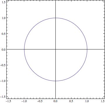
Figure 2: The unit circle.

However, by converting (3) into the homogeneous version (1), we obtain the parametrization

$$\begin{array}[]{cccc}\phi:&\mathbb{P}^{1}&\longrightarrow&\mathbb{P}^{2}\\ &(t_{0}:t_{1})&\longmapsto&\big{(}t_{0}^{2}+t_{1}^{2}:t_{0}^{2}-t_{1}^{2}:2t_{0}t_{1}\big{)},\end{array}$$ (4)

which is well defined on all $\mathbb{P}^{1}.$ Moreover, every point of the circle (in projective coordinates) is in the image of $\phi$, for instance $(1:-1:0)=\phi(0:1),$ which is the point in ${\mathcal{C}}$ we were “missing” from the parametrization (3). The defining polynomial of ${\mathcal{C}}$ in this case is clearly $F(X_{0},X_{1},X_{2})=X_{1}^{2}+X_{2}^{2}-X_{0}^{2}.$

In general, the solution to the implicitization problem involves tools from Elimination Theory, as explained in [CLO07]: from the equation

$$(X_{0}:X_{1}:X_{2})=\big{(}u_{0}(t_{0}:t_{1}):u_{1}(t_{0}:t_{1}):u_{2}(t_{0}:t_{1})\big{)},$$

one “eliminates” the variables $t_{0}$ and $t_{1}$ to get an expression involving only the $X$’s variables.

The elimination process can be done with several tools. The most popular and general is provided by Gröbner bases, as explained in [AL94] (see also [CLO07]). In the case of a rational parametrization like the one we are handling here, we can consider a more efficient and suitable tool: the Sylvester resultant of two homogeneous polynomials in $t_{0},\,t_{1},$ as defined in [AJ06] (see also [CLO05]). We will denote this resultant with $\mbox{\rm Res}_{t_{0},t_{1}}(\cdot,\cdot).$ The following result can be deduced straightforwardly from the section of Elimination and Implicitization in [CLO07].

Proposition 1

There exist $\alpha,\,\beta\in\mathbb{N}$ such that -up to a nonzero constant-

$$\mbox{\rm Res}_{t_{0},t_{1}}\big{(}X_{2}u_{0}(t_{0},t_{1})-X_{0}u_{2}(t_{0},t_{1}),X_{2}u_{1}(t_{0},t_{1})-X_{1}u_{2}(t_{0},t_{1})\big{)}=X_{2}^{\alpha}F(X_{0},X_{1},X_{2})^{\beta}.$$ (5)

Note that as the polynomial $F(X_{0},X_{1},X_{2})$ is well-defined up to a nonzero constant, all formulae involving it must also hold this way. For instance, an explicit computation of (2.3) in Example 1 shows that this resultant is equal to

$$-4X_{2}^{2}\big{(}X_{0}^{2}-X_{1}^{2}-X_{2}^{2}\big{)}.$$ (6)

One may think that the number $-4$ which appears above is just a random constant, but indeed it is indicating us something very important: if the characteristic of $\mathbb{K}$ is $2,$ then it is easy to verify that (3) does not describe a circle, but the line $X_{2}=0.$ What is even worse, (4) is not the parametrization of a curve, as its image is just the point $(1:1:0).$

To compute the Sylvester Resultant one can use the well-known Sylvester matrix (see [AJ06, CLO07]), whose nonzero entries contain coefficients of the two polynomials $X_{2}u_{0}(t_{0},t_{1})-X_{0}u_{2}(t_{0},t_{1})$ and $X_{2}u_{1}(t_{0},t_{1})-X_{1}u_{2}(t_{0},t_{1}),$ regarded as polynomials in the variables $t_{0}$ and $t_{1}$. The resultant is then the determinant of that (square) matrix.

For instance, in Example 1, we have

$$\begin{array}[]{lcl}X_{2}\,u_{0}(t_{0},t_{1})-X_{0}\,u_{2}(t_{0},t_{1})&=&X_{2}t_{0}^{2}-2X_{0}t_{0}t_{1}+X_{2}t_{1}^{2}\\ X_{2}\,u_{1}(t_{0},t_{1})-X_{1}\,u_{2}(t_{0},t_{1})&=&X_{2}t_{0}^{2}-2X_{1}t_{0}t_{1}-X_{2}t_{1}^{2},\end{array}$$

and (6) is obtained as the determinant of the Sylvester matrix

$$\left(\begin{array}[]{rrrr}X_{2}&-2X_{0}&X_{2}&0\\ 0&X_{2}&-2X_{0}&X_{2}\\ X_{2}&-2X_{1}&-X_{2}&0\\ 0&X_{2}&-2X_{1}&-X_{2}\end{array}\right).$$ (7)

Having $X_{2}$ as a factor in (5) is explained by the fact that the polynomials whose resultant is being computed in (2.3) are not completely symmetric in the $X$’s parameters, and indeed $X_{2}$ is the only $X$-monomial appearing in both expansions.

The exponent $\beta$ in (5) has a more subtle explanation, it is the tracing index of the map $\phi$, or the cardinality of its generic fiber. Geometrically, for all but a finite number of points $(p_{0}:p_{1}:p_{2})\in{\mathcal{C}},\,\beta$ is the cardinality of the set $\phi^{-1}(p_{0}:p_{1}:p_{2}).$ Algebraically, it is defined as the degree of the extension

$$\left[\mathbb{K}\big{(}u_{0}(t_{0},t_{1})/u_{2}(t_{0},t_{1}),u_{1}(t_{0},t_{1})/u_{2}(t_{0},t_{1})\big{)}:\,\mathbb{K}(t_{0}/t_{1})\right].$$

In the applications, one already starts with a map $\phi$ as in (1) which is generically injective, i.e. with $\beta=1.$ This assumption is not a big one, due to the fact that generic parametrizations are generically injective, and moreover, thanks to Luröth’s theorem (see [vdW66]), every parametrization $\phi$ as in (1) can be factorized as $\phi=\overline{\phi}\circ\,{\mathcal{P}},$ with $\overline{\phi}:\mathbb{P}^{1}\to\mathbb{P}^{2}$ generically injective, and ${\mathcal{P}}:\mathbb{P}^{1}\to\mathbb{P}^{1}$ being a map defined by a pair of coprime homogeneous polynomial both of them having degree $\beta.$ One can then regard $\overline{\phi}$ as a “reparametrization” of ${\mathcal{C}}$, and there are very efficient algorithms to deal with this problem, see for instance [SWP08].

In closing this section, we should mention the difference between “algebraic (plane) curves” and the rational curves introduced above. An algebraic plane curve is a subset of $\mathbb{P}^{2}$ defined by the zero set of a homogeneous polynomial $G(X_{0},X_{1},X_{2})$. In this sense, any rational plane curve is algebraic, as we can find its defining equation via the implicitization described above. But not all algebraic curve is rational, and moreover, if the curve has degree $3$ or more, a generic algebraic curve will not be rational. Being rational or not is actually a geometric property of the curve,and one should not expect to detect it from the form of the defining polynomial, see [SWP08] for algorithms to decide whether a given polynomial $G(X_{0},X_{1},X_{2})$ defines a rational curve or not.

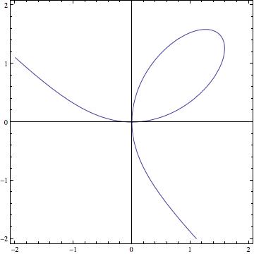
Figure 3: The Folium of Descartes.

For instance, the Folium of Descartes (see Figure 3) is a rational curve with parametrization

$$(t_{0}:t_{1})\mapsto(t_{0}^{3}+t_{1}^{3}:3t_{0}^{2}t_{1}:3t_{0}t_{1}^{2}),$$

and implicit equation given by the polynomial $F(X_{0},X_{1},X_{2})=X_{1}^{3}+X_{2}^{3}-3X_{0}X_{1}X_{2}.$ On the other hand, Fermat’s cubic plotted in Figure 4 is defined by the vanishing of $G(X_{0},X_{1},X_{2})=X_{1}^{3}+X_{2}^{3}-X_{0}^{3}$ but it is not rational.

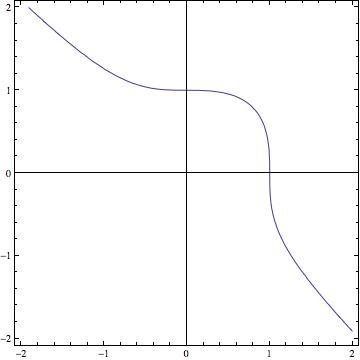
Figure 4: Fermat’s cubic.

The reason why rational curves play a central role in Visualization and Computer Design should be easy to get, as they are

• easy to “manipulate” and be plotted,

• enough to describe all possible kind of shape by using patches (so-called spline curves).

2 Moving lines and $\mu$-bases

Moving lines were introduced by Thomas W. Sederberg and his collaborators in the nineties, [STD94, SC95, SGD97, CSC98]. The idea is the following: in each row of the Sylvester matrix appearing in (7) one can find the coefficients as a polynomial in $t_{0},\,t_{1}$ of a form ${\mathcal{L}}(t_{0},t_{1},X_{0},X_{1},X_{2})\in\mathbb{K}[t_{0},t_{1},X_{0},X_{1},X_{2}]$ of degree $3$ in the variables $t$’s, and satisfying:

$${\mathcal{L}}\big{(}t_{0},t_{1},u_{0}(t_{0},t_{1}),u_{1}(t_{0},t_{1}),u_{2}(t_{0},t_{1})\big{)}=0.$$ (8)

The first row of (7) for instance, contains the coefficients of

$$t_{0}(X_{2}\,u_{0}(t_{0},t_{1})-X_{0}\,u_{2}(t_{0},t_{1}))={\bf X_{2}}t_{0}^{3}{-\bf 2X_{0}}t_{0}^{2}t_{1}+{\bf X_{2}}t_{0}t_{1}^{2}+{\bf 0}t_{1}^{3},$$

which clearly vanishes if we set $X_{i}\mapsto u_{i}(t_{0},t_{1}).$ Note that all the elements in (7) are linear in the $X$’s variables.

With this interpretation in mind, we can regard any such ${\mathcal{L}}(t_{0},t_{1},X_{0},X_{1},X_{2})$ as a family of lines in $\mathbb{P}^{2}$ in such a way that for any $(t_{0}:t_{1})\in\mathbb{P}^{1},$ this line passes through the point $\phi(t_{0}:t_{1})\in{\mathcal{C}}.$ Motivated by this idea, the following central object in this story has been defined.

Definition 1

A moving line of degree $\delta$ which follows the parametrization $\phi$ is a polynomial

$${\mathcal{L}}_{\delta}(t_{0},t_{1},X_{0},X_{1},X_{2})=v_{0}(t_{0},t_{1})X_{0}+v_{1}(t_{0},t_{1})X_{1}+v_{2}(t_{0},t_{1})X_{2}\in\mathbb{K}[t_{0},t_{1},X_{0},X_{1},X_{2}],$$

with each $v_{i}$ homogeneous of degree $\delta,\,i=0,1,2$, such that

$${\mathcal{L}}_{\delta}(t_{0},t_{1},u_{0}(t_{0},t_{1}),u_{1}(t_{0},t_{1}),u_{2}(t_{0},t_{1}))=0,$$

i.e.

$$v_{0}(t_{0},t_{1})u_{0}(t_{0},t_{1})+v_{1}(t_{0},t_{1})u_{1}(t_{0},t_{1})+v_{2}(t_{0},t_{1})u_{2}(t_{0},t_{1})=0.$$ (9)

Note that both $X_{2}u_{0}(t_{0},t_{1})-X_{0}u_{2}(t_{0},t_{1})$ and $X_{2}u_{1}(t_{0},t_{1})-X_{1}u_{2}(t_{0},t_{1})$ are always moving lines following $\phi$. Moreover, note that if we multiply any given moving line by a homogeneous polynomial in $\mathbb{K}[t_{0},t_{1}]$, we obtain another moving line of higher degree. The set of moving lines following a given parametrization has an algebraic structure of a module over the ring $\mathbb{K}[t_{0},t_{1}].$ Indeed, another way of saying that ${\mathcal{L}}_{\delta}(t_{0},t_{1},X_{0},X_{1},X_{2})$ is a moving line which follows $\phi$ is that the vector $(v_{0}(t_{0},t_{1}),v_{1}(t_{0},t_{1}),v_{2}(t_{0},t_{1}))$ is a homogeneous element of the syzygy module of the ideal generated by the sequence $\{u_{0}(t_{0},t_{1}),\,u_{1}(t_{0},t_{1}),\,u_{2}(t_{0},t_{1})\}$ -the coordinates of $\phi$- in the ring of polynomials $\mathbb{K}[t_{0},t_{1}].$

We will not go further in this direction yet, as the definition of moving lines does not require understanding concepts like syzygies or modules. Note that computing moving lines is very easy from an equality like (9). Indeed, one first fixes $\delta$ as small as possible, and then sets $v_{0}(t_{0},t_{1}),\,v_{1}(t_{0},t_{1}),\,v_{2}(t_{0},t_{1})$ as homogeneous polynomials of degree $\delta$ and unknown coefficients, which can be solved via the linear system of equations determined by (9).

With this very simple but useful object, the method of implitization by moving lines as stated in [STD94] says essentially the following: look for a set of moving lines of the same degree $\delta,$ with $\delta$ as small as possible, which are “independent” in the sense that the matrix of their coefficients (as polynomials in $t_{0},\,t_{1}$) has maximal rank. If you are lucky enough, you will find $\delta+1$ of these forms, and hence the matrix will be square. Compute then the determinant of this matrix, and you will get a non-trivial multiple of the implicit equation. If your are even luckier, your determinant will be equal to $F(X_{0},X_{1},X_{2})^{\beta}.$

Example 2

Let us go back to the parametrization of the unit circle given in Example 1. We check straightforwardly that both

$$\begin{array}[]{cclcl}{\mathcal{L}}_{1}(t_{0},t_{1},X_{0},X_{1},X_{2})&=&-t_{1}X_{0}-t_{1}X_{1}+t_{0}X_{2}&=&X_{2}\,t_{0}-(X_{0}+X_{1})\,t_{1}\\ {\mathcal{L}}_{2}(t_{0},t_{1},X_{0},X_{1},X_{2})&=&-t_{0}X_{0}+t_{0}X_{1}+t_{1}X_{2}&=&(-X_{0}+X_{1})\,t_{0}+X_{2}\,t_{1}.\end{array}$$

satisfy (8). Hence, they are moving lines of degree $1$ which follow the parametrization of the unit circle. Here, $\delta=1.$ We compute the matrix of their coefficients as polynomials (actually, linear forms) in $t_{0},t_{1}$, and get

$$\left(\begin{array}[]{lr}X_{2}&-X_{0}-X_{1}\\ -X_{0}+X_{1}&X_{2}\end{array}\right).$$ (10)

It is easy to check that the determinant of this matrix is equal to

$$F(X_{0},X_{1},X_{2})=X_{1}^{2}+X_{2}^{2}-X_{0}^{2}.$$

Note that the size of (10) is actually half of the size of (7), and also that the determinant of this matrix gives the implicit equation without any extraneous factor.

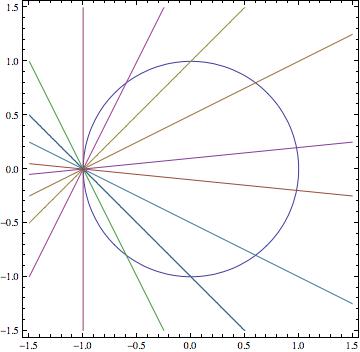
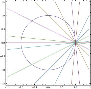
Figure 5: Moving lines ${\mathcal{L}}_{1}$ (left) and ${\mathcal{L}}_{2}$ (right).

Of course, in order to convince the reader that this method is actually better than just performing (5), we must shed some light on how to compute algorithmically a matrix of moving lines. The following result was somehow discovered by Hilbert more than a hundred years ago, and rediscovered in the CAGD community in the late nineties (see [CSC98]).

Theorem 2.1

For $\phi$ as in (1), there exist a unique $\mu\leq\frac{d}{2}$ and two moving lines following $\phi$ which we will denote as ${\mathcal{P}}_{\mu}(t_{0},t_{1},X_{0},X_{1},X_{2}),\,{\mathcal{Q}}_{d-\mu}(t_{0},t_{1},X_{0},X_{1},X_{2})$ of degrees $\mu$ and $d-\mu$ respectively such that any other moving line following $\phi$ is a polynomial combination of these two, i.e. if every ${\mathcal{L}}_{\delta}(t_{0},t_{1},X_{0},X_{1},X_{2})$ as in the Definition 1 can be written as

$${\mathcal{L}}_{\delta}(t_{0},t_{1},X_{0},X_{1},X_{2})=p(t_{0},t_{1}){\mathcal{P}}_{\mu}(t_{0},t_{1},X_{0},X_{1},X_{2})+q(t_{0},t_{1}){\mathcal{P}}_{d-\mu}(t_{0},t_{1},X_{0},X_{1},X_{2}),$$

with $p(t_{0},t_{1}),\,q(t_{0},t_{1})\in\mathbb{K}[t_{0},t_{1}]$ homogeneous of degrees $\delta-\mu$ and $\delta-d+\mu$ respectively.

This statement is consequence of a stronger one, which essentially says that a parametrization $\phi$ as in (1), can be “factorized” as follows:

Theorem 2.2 (Hilbert-Burch)

For $\phi$ as in (1), there exist a unique $\mu\leq\frac{d}{2}$ and two parametrizations $\varphi_{\mu},\,\psi_{d-\mu}:\mathbb{P}^{1}\to\mathbb{P}^{2}$ of degrees $\mu$ and $d-\mu$ respectively such that

$$\phi(t_{0}:t_{1})=\varphi_{\mu}(t_{0}:t_{1})\times\psi_{d-\mu}(t_{0}:t_{1}),$$ (11)

where $\times$ denotes the usual cross product of vectors.

Note that we made an abuse of notation in the statement of (11), as $\varphi_{\mu}(t_{0}:t_{1})$ and $\psi_{d-\mu}(t_{0}:t_{1})$ are elements in $\mathbb{P}^{2}$ and the cross product is not defined in this space. The meaning of $\times$ in (11) should be understood as follows: pick representatives in $\mathbb{K}^{3}$ of both $\varphi_{\mu}(t_{0}:t_{1})$ and $\psi_{d-\mu}(t_{0}:t_{1}),$ compute the cross product of these two representatives, and then “projectivize” the result to $\mathbb{P}^{2}$ again.

The parametrizations $\varphi_{\mu}$ and $\psi_{d-\mu}$ can be explicited by computing a free resolution of the ideal $\langle u_{0}(t_{0},t_{1}),\,u_{1}(t_{0},t_{1}),\,u_{2}(t_{0},t_{1})\rangle\subset\mathbb{K}[t_{0},t_{1}],$ and there are algorithms to do that, see for instance [CDNR97]. Note that even though general algorithms for computing free resolutions are based on computations of Gröbner bases, which have in general bad complexity time, the advantage here is that we are working with a graded resolution, and also that the resolution of an ideal like the one we deal with here is of Hilbert-Burch type in the sense of [Eis95]. This means that the coordinates of both $\varphi_{d}$ and $\psi_{d-\mu}$ appear in the columns of the $2\times 3$ matrix of the first syzygies in the resolution. We refer the reader to [CSC98] for more details on the proofs of Theorems 2.1 and 2.2.

The connection between the moving lines ${\mathcal{P}}_{\mu}(t_{0},t_{1},X_{0},X_{1},X_{2}),\,{\mathcal{Q}}_{d-\mu}(t_{0},t_{1},X_{0},X_{1},X_{2})$ of Theorem (2.1) and the parametrizations $\varphi_{\mu},\,\psi_{d-\mu}$ in (11) is the obvious one: the coordinates of $\varphi_{\mu}$ (resp. $\psi_{d-\mu}$) are the coefficients of ${\mathcal{P}}_{\mu}(t_{0},t_{1},X_{0},X_{1},X_{2})$ (resp. ${\mathcal{Q}}_{d-\mu}(t_{0},t_{1},X_{0},X_{1},X_{2})$) as a polynomial in $X_{0},\,X_{1},\,X_{2}.$

Definition 2

A sequence $\{{\mathcal{P}}_{\mu}(t_{0},t_{1},X_{0},X_{1},X_{2}),\,{\mathcal{Q}}_{d-\mu}(t_{0},t_{1},X_{0},X_{1},X_{2})\}$ as in Theorem 2.1, is called a $\mu$-basis of $\phi.$

Note that both theorems 2.1 and 2.2 only state the uniquenes of the value of $\mu$, and not of ${\mathcal{P}}_{\mu}(t_{0},t_{1},X_{0},X_{1},X_{2})$ and ${\mathcal{Q}}_{d-\mu}(t_{0},t_{1},X_{0},X_{1},X_{2}).$ Indeed, if $\mu=d-\mu$ (which happens generically if $d$ is even), then any two generic linear combinations of the elements of a $\mu$-basis is again another $\mu-$basis. If $\mu<d-\mu,$ then any polynomial multiple of ${\mathcal{P}}_{\mu}(t_{0},t_{1},X_{0},X_{1},X_{2})$ of the proper degree can be added to ${\mathcal{Q}}_{d-\mu}(t_{0},t_{1},X_{0},X_{1},X_{2})$ to produce a different $\mu$-basis of the same parametrization.

Example 3

For the parametrization of the unit circle given in Example 1, one can easily check that

$$\begin{array}[]{lcl}\varphi_{1}(t_{0}:t_{1})&=&(-t_{1}:-t_{1}:t_{0}),\\ \psi_{1}(t_{0}:t_{1})&=&(-t_{0}:t_{0}:t_{1})\end{array}$$

is a $\mu$-basis of $\phi$ defined in (4), i.e. this parametrization has $\mu=d-\mu=1.$ Indeed, we compute the cross product in (11) as follows: denote with ${\boldsymbol{e}}_{0},\,{\boldsymbol{e}}_{1},\,{\boldsymbol{e}}_{2}$ the vectors of the canonical basis of $\mathbb{K}^{3}$. Then, we get

$$\left|\begin{array}[]{rrr}{\boldsymbol{e}}_{0}&{\boldsymbol{e}}_{1}&{\boldsymbol{e}}_{2}\\ -t_{1}&t_{1}&t_{0}\\ -t_{0}&t_{0}&t_{1}\end{array}\right|=\big{(}-t_{0}^{2}-t_{1}^{2},\,t_{1}^{2}-t_{0}^{2},\,-2t_{0}t_{1}\big{)},$$

which shows that the $\varphi_{1}(t_{0}:t_{1})\times\psi_{1}(t_{0}:t_{1})=\phi(t_{0}:t_{1}),$ according to (11).

The reason the computation of $\mu$-bases is important, is not only because with them we can generate all the moving lines which follow a given parametrization, but also because they will allow us to produce small matrices of moving lines whose determinant give the implicit equation. Indeed, the following result has been proven in [CSC98, Theorem 1].

Theorem 2.3

With notation as above, let $\beta$ be the tracing index of $\phi.$ Then, up to a nonzero constant in $\mathbb{K}$, we have

$$\mbox{\rm Res}_{t_{0},t_{1}}\big{(}{\mathcal{P}}_{\mu}(t_{0},t_{1},X_{0},X_{1},X_{2}),{\mathcal{Q}}_{d-\mu}(t_{0},t_{1},X_{0},X_{1},X_{2})\big{)}=F(X_{0},X_{1},X_{2})^{\beta}.$$ (12)

As shown in [SGD97] if you use any kind of matrix formulation for computing the Sylvester resultant, in each row of these matrices, when applied to formulas (5) and (12), you will find the coefficients (as a polynomial in $t_{0},\,t_{1}$) of a moving line following the parametrization. Note that the formula given by Theorem 2.3 always involves a smaller matrix than the one in (5), as the $t$-degrees of the polynomials ${\mathcal{P}}_{\mu}(t_{0},t_{1},X_{0},X_{1},X_{2})$ and ${\mathcal{Q}}_{d-\mu}(t_{0},t_{1},X_{0},X_{1},X_{2})$ are roughly half of the degrees of those in (5).

There is, of course, a connection between these two formulas. Indeed, denote with $\mbox{\rm Syl}_{t_{0},t_{1}}(G,H)$ (resp. $\mbox{\rm Bez}_{t_{0},t_{1}}(G,H)$) the Sylvester (resp. Bézout) matrix for computing the resultant of two homogeneous polynomials of $G,H\in\mathbb{K}[t_{0},t_{1}].$ For more about definitions and properties of these matrices, see [AJ06]. In [BD12, Proposition 6.1], we prove with Laurent Busé the following:

Theorem 2.4

There exists an invertible matrix $M\in\mathbb{K}^{d\times d}$ such that

$$\begin{array}[]{l}X_{2}\cdot\,\mbox{\rm Sylv}_{t_{0},t_{1}}\big{(}{\mathcal{P}}_{\mu}(t_{0},t_{1},X_{0},X_{1},X_{2}),{\mathcal{Q}}_{d-\mu}(t_{0},t_{1},X_{0},X_{1},X_{2})\big{)}\\ =M\cdot\,\mbox{\rm Bez}_{t_{0},t_{1}}\big{(}X_{2}u_{0}(t_{0},t_{1})-X_{0}u_{2}(t_{0},t_{1}),X_{2}u_{1}(t_{0},t_{1})-X_{1}u_{2}(t_{0},t_{1})\big{)}.\end{array}$$

From the identity above, one can easily deduce that it is possible to compute the implicit equation (or a power of it) of a rational parametrization with a determinant of a matrix of coefficients of $d$ moving lines, where $d$ is the degree of $\phi$. Can you do it with less? Unfortunately, the answer is no, as each row or column of a matrix of moving lines is linear in $X_{0},X_{1},X_{2},$ and the implicit equation has typically degree $d.$ So, the method will work optimally with a matrix of size $d\times d$, and essentially you will be computing the Sylvester matrix of a $\mu$-basis of $\phi$.

3 Moving conics, moving cubics…

One can actually take advantage of the resultant formulation given in (12) and get a determinantal formula for the implicit equation by using the square matrix

$$\mbox{\rm Bez}_{t_{0},t_{1}}\big{(}{\mathcal{P}}_{\mu}(t_{0},t_{1},X_{0},X_{1},X_{2}),{\mathcal{Q}}_{d-\mu}(t_{0},t_{1},X_{0},X_{1},X_{2})\big{)},$$

which has smaller size (it will have $d-\mu$ rows and columns) than the Sylvester matrix of these polynomials. But this will not be a matrix of coefficients of moving lines anymore, as the input coefficients of the Bézout matrix will be quadratic in $X_{0},\,X_{1},\,X_{2}.$ Yet, due to the way the Bézout matrix is being built (see for instance [SGD97], one can find in the rows of this matrix the coefficients of a polynomial which also vanishes on the parametrization $\phi.$ This motivates the following definition:

Definition 3

A moving curve of bidegree $(\nu,\delta)$ which follows the parametrization $\phi$ is a polynomial ${\mathcal{L}}_{\nu,\delta}(t_{0},t_{1},X_{0},X_{1},X_{2})\in\mathbb{K}[t_{0},t_{1},X_{0},X_{1},X_{2}]$ homogeneous in $X_{0},\,X_{1},\,X_{2}$ of degree $\nu$ and in $t_{0},\,t_{1}$ of degree $\delta,$ such that

$${\mathcal{L}}\big{(}t_{0},t_{1},u_{0}(t_{0},t_{1}),u_{1}(t_{0},t_{1}),u_{2}(t_{0},t_{1})\big{)}=0.$$

If $\nu=1$ we recover the definition of moving lines given in (1). For $\nu=2,$ the polynomial ${\mathcal{L}}(t_{0},t_{1},X_{0},X_{1},X_{2})$ is called a moving conic which follows $\phi$ ([ZCG99]). Moving cubics will be curves with $\nu=3,$ and so on.

A series of experiments made by Sederberg and his collaborators showed something interesting: one can compute the defining polynomial of ${\mathcal{C}}$ as a determinant of a matrix of coefficients of moving curves following the parametrization, but the more singular the curve is (i.e. the more singular points it has), the smaller the determinant of moving curves gets. For instance, the following result appears in [SC95]:

Theorem 3.1

The implicit equation of a quartic curve with no base points can be written as a $2\times 2$ determinant. If the curve doesn’t have a triple point, then each element of the determinant is a quadratic; otherwise one row is linear and one row is cubic.

To illustrate this, we consider the following examples.

Example 4

Set $u_{0}(t_{0},t_{1})=t_{0}^{4}-t_{1}^{4},\,u_{1}(t_{0},t_{1})=-t_{0}^{2}t_{1}^{2},u_{2}(t_{0},t_{1})=t_{0}t_{1}^{3}.$ These polynomials defined a parametrization $\phi$ as in (1) with implicit equation given by the polynomial $F(X_{0},X_{1},X_{2})=X_{2}^{4}-X_{1}^{4}-X_{0}X_{1}X_{2}^{2}.$ From the shape of this polynomial, it is easy to show that $(1:0:0)\in\mathbb{P}^{2}$ is a point of multiplicity $3$ of this curve, see Figure 6. In this case, we have $\mu=1,$ and it is also easy to verify that

$${\mathcal{L}}_{1,1}(t_{0},t_{1},X_{0},X_{1},X_{2})=t_{0}X_{2}+t_{1}X_{1}$$

is a moving line which follows $\phi$. The reader will now easily check that the following moving curve of bidegree $(3,1)$ also follows $\phi$:

$${\mathcal{L}}_{1,3}(t_{0},t_{1},X_{0},X_{1},X_{2})=t_{0}(X_{1}^{3}+X_{0}X_{2}^{2})+t_{1}\,X_{2}^{3}.$$

And the $2\times 2$ matrix claimed in Theorem 3.1 for this case is made with the coefficients of both ${\mathcal{L}}_{1,1}(t_{0},t_{1},X_{0},X_{1},X_{2})$ and ${\mathcal{L}}_{1,3}(t_{0},t_{1},X_{0},X_{1},X_{2})$ as polynomials in $t_{0},\,t_{1}:$

$$\left(\begin{array}[]{lr}X_{2}&X_{1}\\ X_{1}^{3}+X_{0}X_{2}^{2}&X_{2}^{3}\end{array}\right).$$

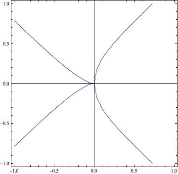
Figure 6: The curve of Example 4.

Example 5

We reproduce here Example 2.7 in [Cox08]. Consider

$$u_{0}(t_{0},t_{1})=t_{0}^{4},\,u_{1}(t_{0},t_{1})=6t_{0}^{2}t_{1}^{2}-4t_{1}^{4},\,u_{2}(t_{0},t_{1})=4t_{0}^{3}t_{1}-4t_{0}t_{1}^{3}.$$

This input defines a quartic curve with three nodes, with implicit equation given by
$F(X_{0},X_{1},X_{2})=X_{2}^{4}+4X_{0}X_{1}^{3}+2X_{0}X_{1}X_{2}^{2}-16X_{0}^{2}X_{1}^{2}-6X_{0}^{2}X_{2}^{2}+16X_{0}^{3}X_{1},$ see Figure 7.

The following two moving conics of degree $1$ in $t_{0},\,t_{1}$ follow the parametrization:

$$\begin{array}[]{ccl}{\mathcal{L}}_{1,2}(t_{0},t_{1},X_{0},X_{1},X_{2})&=&t_{0}(X_{1}X_{2}-X_{0}X_{2})+t_{1}(-X_{2}^{2}-2X_{0}X_{1}+4X_{0}^{2})\\ \tilde{{\mathcal{L}}}_{1,2}(t_{0},t_{1},X_{0},X_{1},X_{2})&=&t_{0}(X_{1}^{2}+\frac{1}{2}X_{2}^{2}-2X_{0}X_{1})+t_{1}(X_{0}X_{2}-X_{1}X_{2}).\end{array}$$

As in the previous example, the $2\times 2$ matrix of the coefficients of these moving conics is the matrix claimed in Theorem 3.1.

Figure 7: The curve of Example 5.

4 The moving curve ideal of $\phi$

Now it is time to introduce some tools from Algebra which will help us understand all the geometric constructions defined above.The set of all moving curves following a given parametrization generates a bi-homogeneous ideal in $\mathbb{K}[t_{0},t_{1},X_{0},X_{1},X_{2}]$, which we will call the moving curve ideal of this parametrization.

As explained above, the method of moving curves for implicitization of a rational parametrization looks for small determinants made with coefficients of moving curves which follow the parametrization of low degree in $t_{0},\,t_{1}.$ To do this, one would like to have a description as in Theorem 2.1, of a set of “minimal” moving curves from which we can describe in an easy way all the other elements of the moving curve ideal.

Fortunately, Commutative Algebra provides the adequate language and tools for dealing with this problem. As it was shown by David Cox in [Cox08], all we have to do is look for minimal generators of the kernel ${\mathcal{K}}$ of the following morphism of rings:

$$\begin{array}[]{cclr}\mathbb{K}[t_{0},t_{1},X_{0},X_{1},X_{2}]&\longrightarrow&\mathbb{K}[t_{0},t_{1},z]\\ t_{i}&\longmapsto&t_{i}&\,i=0,1,\\ X_{j}&\longmapsto&u_{j}(t_{0},t_{1})\,z&\,j=0,1,2.\end{array}$$ (13)

Here, $z$ is a new variable. The following result appears in [Cox08, Nice Fact 2.4] (see also [BJ03] for the case when $\phi$ is not generically injective):

Theorem 4.1

${\mathcal{K}}$ is the moving curve ideal of $\phi$ .

Let us say some words about the map (13). Denote with $I\subset\mathbb{K}[t_{0},\,t_{1}]$ the ideal generated by $u_{0}(t_{0},t_{1}),\,u_{1}(t_{0},t_{1}),\,u_{2}(t_{0},t_{1})$. The image of (13) is actually isomorphic to $\mathbb{K}[t_{0},t_{1}][z\,I],$ which is called the Rees Algebra of $I$. By the Isomorphism Theorem, we then get that $\mathbb{K}[t_{0},t_{1},X_{0},X_{1},X_{2}]/{\mathcal{K}}$ is isomorphic to the Rees Algebra of $I$. This is why the generators of ${\mathcal{K}}$ are called the defining equations of the Rees Algebra of $I$. The Rees Algebra that appears in the moving lines method corresponds to the blow-up of $V(I),$ the variety defined by $I$. Geometrically, it is is just the blow-up of the empty space (the effect of this blow-up is just to introduce torsion…), but yet the construction should explain somehow why moving curves are sensitive to the presence of complicated singularities. It is somehow strange that the fact that the description of ${\mathcal{K}}$ actually gets much simpler if the singularities of ${\mathcal{C}}$ are more entangled.

Let us show this with an example. It has been shown in [Bus09], by unravelling some duality theory developed by Jouanolou in [Jou97], that for any proper parametrization of a curve of degree $d$ having $\mu=2$ and only cusps as singular points, the kernel ${\mathcal{K}}$ has $\frac{(d+1)(d-4)}{2}+5$ minimal generators. On the other hand, in a joint work with Teresa Cortadellas [CD13b] (see also [KPU13]), we have shown that if $\mu=2$ and there is a point of very high multiplicity (it can be proven that if the multiplicity of a point is larger than $3$ when $\mu=2$, then it must be equal to $d-2$), then the number of generators drops to $\lfloor\frac{d+6}{2}\rfloor,$ i.e. the description of ${\mathcal{K}}$ is simpler in this case. In both cases, these generators can be make explicit, see [Bus09, CD13b, KPU13].

Further evidence supporting this claim is what is already known for the case $\mu=1$, which was one of the first one being worked out by several authors: [HSV08, CHW08, Bus09, CD10]. It turns out (cf. [CD10, Corollary 2.2]) that $\mu=1$ if and only if the parametrization is proper (i.e. generically injective), and there is a point on ${\mathcal{C}}$ which has multiplicity $d-1$, which is the maximal multiplicity a point can have on a curve of degree $d.$ If this is the case, then the parametrization has exactly $d+1$ elements.

In both cases ($\mu=1$ and $\mu=2$), explicit elements of a set of minimal generators of ${\mathcal{K}}$ can be given in terms of the input parametrization. But in general, very little is known about how many are them and which are their bidegrees. Let $n_{0}({\mathcal{K}})$ be the $0$-th Betti number of ${\mathcal{K}}$ (i.e.  the cardinal of any minimal set of generators of ${\mathcal{K}}$). We propose the following problem which is the subject of attention of several researchers at the moment.

Problem 1

Describe all the possible values of $n_{0}({\mathcal{K}})$ and the parameters that this function depends on, for a proper parametrization $\phi$ as in (1).

Recall that “proper” here means “generically injective”. For instance, we just have shown above that, for $\mu=1,\,n_{0}(\mu)=d+1.$ If $\mu=2,$ the value of $n_{0}({\mathcal{K}})$ depends on whether there is a very singular point or not. Is $n_{0}$ a function of only $d,\,\mu$ and the multiplicity structure of ${\mathcal{C}}$?

A more ambitious problem of course is the following. Let ${\mathcal{B}}({\mathcal{K}})\subset\mathbb{N}^{2}$ be the (multi)-set of bidegrees of a minimal set of generators of ${\mathcal{K}}$.

Problem 2

Describe all the possible values of ${\mathcal{B}}({\mathcal{K}}).$

For instance, if $\mu=1,$ we have that (see [CD10, Theorem 2.9])

$${\mathcal{B}}({\mathcal{K}})=\{(0,d),\,(1,1),\,(1,d-1),\,(2,d-2),\ldots,(d-1,1)\}.$$

Explicit descriptions of ${\mathcal{B}}({\mathcal{K}})$ have been done also for $\mu=2$ in [Bus09, CD13b, KPU13]. In this case, the value of ${\mathcal{B}}({\mathcal{K}})$ depends on whether the parametrization has singular point of multiplicity $d-2$ or not.

For $\mu=3$ the situation gets a bit more complicated as we have found in [CD13b]: consider the parametrizations $\phi_{1}$ and $\phi_{2}$ whose $\mu$-bases are respectively :

$$\begin{array}[]{l}{\mathcal{P}}_{3,1}(t_{0},t_{1},X_{0},X_{1},X_{2})=t_{0}^{3}X_{0}+(t_{1}^{3}-t_{0}t_{1}^{2})X_{1}\\ {\mathcal{Q}}_{7,1}(t_{0},t_{1},X_{0},X_{1},X_{2})=(t_{0}^{6}t_{1}-t_{0}^{2}t_{1}^{5})X_{0}+(t_{0}^{4}t_{1}^{3}+t_{0}^{2}t_{1}^{5})X_{1}+(t_{0}^{7}+t_{1}^{7})X_{2},\\ \\ {\mathcal{P}}_{3,2}(t_{0},t_{1},X_{0},X_{1},X_{2})=(t_{0}^{3}-t_{0}^{2}t_{1})X_{0}+(t_{1}^{3}+t_{0}t_{1}^{2}-t_{0}^{2}t_{1})X_{1}\\ {\mathcal{Q}}_{7,2}(t_{0},t_{1},X_{0},X_{1},X_{2})=(t_{0}^{6}t_{1}-t_{0}^{2}t_{1}^{5})X_{0}+(t_{0}^{4}t_{1}^{3}+t_{0}^{2}t_{1}^{5})X_{1}+(t_{0}^{7}+t_{1}^{7})X_{2}.\end{array}$$

Each of them parametrizes properly a rational plane curve of degree $10$ having the point $(0:0:1)$ with multiplicity 7. The rest of them are either double or triple points. Set ${\mathcal{K}}_{1}$ and ${\mathcal{K}}_{2}$ for the respective kernels, we have then

$$\begin{array}[]{rcl}{\mathcal{B}}({\mathcal{K}}_{1})&=&\{(3,1),\,(7,1),\,(2,3),\,(2,3),\,(4,2),\,(2,4),\,(1,6),\,(1,6),\,(1,6),\,(0,10)\},\\ {\mathcal{B}}({\mathcal{K}}_{2})&=&\{(3,1),\,(7,1),\,(2,3),\,(2,3),\,(4,2),\,(2,4),\,{\bf(1,5)},\,(1,6),\,(1,6),\,(0,10)\}.\end{array}$$

The parameters to find in the description of $n_{0}({\mathcal{K}})$ proposed in Problem 1 may be more than $\mu$ and the multiplicities of the curve. For instance, in [CD13], we have shown that if there is a minimal generator of bidegree $(1,2)$ in ${\mathcal{K}},$ then the whole set ${\mathcal{B}}({\mathcal{K}})$ is constant, and equal to

$$\left\{\begin{array}[]{lrc}\{(0,d),\,(1,2),\,(1,d-2),\,(2,d-4),\ldots,(\frac{d-1}{2},1),\,(\frac{d+1}{2},1)\}&&\mbox{if}\,d\,\mbox{is odd}\\ \{(0,d),\,(1,2),\,(1,d-2),\,(2,d-4),\ldots,(\frac{d}{2},1),\,(\frac{d}{2},1)\}&&\mbox{if}\,d\,\mbox{is even.}\end{array}\right.$$

To put the two problems above in a more formal context, we proceed as in [CSC98, Section 3]: For $d\geq 1,$ denote with $\mathbb{V}_{d}\subset{\mathbb{K}[t_{0},t_{1}]_{d}}^{3}$ the set of triples of homogeneous polynomials $(u_{0}(t_{0},t_{1}),\,u_{1}(t_{0},t_{1}),\,u_{2}(t_{0},t_{1})\big{)}$ defining a proper parametrization $\phi$ as in (1). Note that one can regard $\mathbb{V}_{d}$ as an open set in an algebraic variety in the space of parameters. Moreover, $\mathbb{V}_{d}$ could be actually be taken as a quotient of ${\mathbb{K}[t_{0},t_{1}]_{d}}^{3}$ via the action of $\mbox{SL}(2,\mathbb{K})$ acting on the monomials $t_{0},\,t_{1}$.

Problem 3

Describe the subsets of $\mathbb{V}_{d}$ where ${\mathcal{B}}({\mathcal{K}})$ is constant.

Note that, naturally the $\mu$-basis is contained in ${\mathcal{K}},$ and moreover, we have (see [BJ03, Proposition 3.6]):

$${\mathcal{K}}=\langle{\mathcal{P}}_{\mu}(t_{0},t_{1},X_{0},X_{1},X_{2}),\,{\mathcal{Q}}_{d-\mu}(t_{0},t_{1},X_{0},X_{1},X_{2})\rangle:\langle t_{0},\,t_{1}\rangle^{\infty},$$

so the role of the $\mu$-basis is crucial to understand ${\mathcal{K}}$. Indeed, any minimal set of generators of ${\mathcal{K}}$ contains a $\mu$-basis, so the pairs $(1,\mu),\,(1,d-\mu)$ are always elements of $B({\mathcal{K}}).$ The study of the geometry of $\mathbb{V}_{d}$ according to the stratification done by $\mu$ has been done in [CSC98, Section 3] (see also [DAn04, Iar13]). Also, in [CKPU13], a very interesting study of how the $\mu$-basis of a parametrization having generic $\mu$ ($\mu=\lfloor d/2\rfloor$) and very singular points looks like has been made. It would be interesting to have similar results for ${\mathcal{K}}$.

In this context, one could give a positive answer to the experimental evidence provided by Sederberg and his collaborators about the fact that “the more singular the curve, the simpler the description of $K$” as follows. For $\mathbb{W}\subset\mathbb{V}_{d}$, we denote by $\overline{\mathbb{W}}$ the closure of $\mathbb{W}$ with respect to the Zariski topology.

Conjecture 1

If $\mathbb{W}_{1},\,\mathbb{W}_{2}\subset\mathbb{V}_{d}$ are such that $n_{0}|_{\mathbb{W}_{i}}$ is constant for $i=1,2,$ and $\overline{\mathbb{W}}_{1}\subset\overline{\mathbb{W}}_{2},$ then

$$n_{0}\big{(}\mathbb{W}_{1}\big{)}\leq n_{0}\big{(}\mathbb{W}_{2}\big{)}.$$

Note that this condition is equivalent to the fact that $n_{0}({\mathcal{K}})$ is upper semi-continuous on $\mathbb{V}_{d}$ with its Zariski topology. Very related to this conjecture is the following claim, which essentially asserts that in the “generic” case, we obtain the largest value of $n_{0}({\mathcal{K}}):$

Conjecture 2

Let $\mathbb{W}_{d}$ be open set of $\mathbb{V}_{d}$ parametrizing all the curves with $\mu=\lfloor d/2\rfloor,$ and having all its singular points being ordinary double points. Then, $n_{0}({\mathcal{K}})$ is constant on $\mathbb{W}_{d},$ and attains its maximal value on $\mathbb{V}_{d}$ in this component.

Note that a “refinement” of Conjecture 1 with ${\mathcal{B}}({\mathcal{K}}_{1})\subset{\mathcal{B}}({\mathcal{K}}_{2})$ will not hold in general, as in the examples computed for $\mu=2$ in [Bus09, CD13b, KPU13] show. Indeed, we have in this case that the Zariski closure of those parametrizations with a point of multiplicity $d-2$ is contained in the case where all the points are only cusps, but the bidegrees of the minimal generators of ${\mathcal{K}}$ in the case of parametrizations with points of multiplicity $d-2$ appear at lower values than the more general case (only cusps).

5 Why Rational Plane Curves only?

All along this text we were working with the parametrization of a rational plane curve, but most of the concepts, methods and properties worked out here can be extended in two different directions. The obvious one is to consider “surface” parametrizations, that is maps of the form

$$\begin{array}[]{cccc}\phi_{S}:&\mathbb{P}^{2}&\dasharrow&\mathbb{P}^{3}\\ &(t_{0}:t_{1}:t_{2})&\longmapsto&\big{(}u_{0}(t_{0},t_{1},t_{2}):u_{1}(t_{0},t_{1},t_{2}):u_{2}(t_{0},t_{1},t_{2}):u_{3}(t_{0},t_{1},t_{2})\big{)}\end{array}$$ (14)

where $u_{i}(t_{0},t_{1},t_{2})\in\mathbb{K}[t_{0},t_{1},t_{2}],\,i=0,1,2,3,$ are homogeneous of the same degree, and without common factors. Obviously, one can do this in higher dimensions also, but we will restrict the presentation just to this case. The reason we have now a dashed arrow in (14) is because even with the conditions imposed upon the $u_{i}$’s, the map may not be defined on all points of $\mathbb{P}^{2}.$ For instance, if

$$u_{0}(t_{0},t_{1},t_{2})=t_{1}t_{2},\,u_{1}(t_{0},t_{1},t_{2})=t_{0}t_{2},\,u_{2}(t_{0},t_{1},t_{2})=t_{0}t_{1},\,u_{3}(t_{0},t_{1},t_{2})=t_{0}t_{1}+t_{1}t_{2},$$

$\phi_{S}$ will not be defined on the set $\{(1:0:0),\,(0:1:0),\,(0:0:1)\}.$

In this context, there are methods to deal with the implicitization analogues to those presented here for plane curves. For instance, one can use a multivariate resultant or a sparse resultant (as defined in [CLO05]) to compute the implicit equation of the Zariski closure of the image of $\phi_{S}$. Other tools from Elimination Theory such as determinants of complexes can be also used to produce matrices whose determinant (or quotient or $\gcd$ of some determinants) can also be applied to compute the implicit equation, see for instance [BJ03, BCJ09].

The method of moving lines and curves presented before gets translated into a method of moving planes and surfaces which follows $\phi_{S}$, and its description and validity is much more complicated, as the both the Algebra and the Geometry involved have more subtleties, see [SC95, CGZ00, Cox01, BCD03, KD06]. Even though it has been shown in [CCL05] that there exists an equivalent of a $\mu$-basis in this context, its computation of is not as easy as in the planar case. Part of the reason is that the syzygy module of general $u_{i}(t_{0},t_{1},t_{2}),\,i=0,1,2,3$ is not free anymore (i.e. it does not have sense the meaning of a “basis” as we defined in the case of curves), but if one set $t_{0}=1$ and regards these polynomials as affine bivariate forms, a nicer situation appears but without control on the degrees of the elements of the $\mu$-basis, see [CCL05, Proposition 2.1] for more on this. Some explicit descriptions have been done for either low degree parametrizations, and also for surfaces having some additional geometric features (see [CSD07, WC12, SG12, SWG12]), but the general case remains yet to be explored.

A generalization of a map like (13) to this situation is straightforward, and one can then consider the defining ideal of the Rees Algebra associated to $\phi_{S}$. Very little seems to be known about the minimal generators of ${\mathcal{K}}$ in this situation. In [CD10] we studied the case of monoid surfaces, which are rational parametrizations with a point of the highest possible multiplicity. This situation can be regarded as a possible generalization of the case $\mu=1$ for plane curves, and has been actually generalized to de Jonquières parametrizations in [HS12].

We also dealt in [CD10] (see also [HW10]) with the case where there are two linearly independent moving planes of degree $1$ following the parametrization plus some geometric conditions, this may be regarded of a generalization of the “$\mu=1$” situation for plane curves. But the general description of the defining ideal of the Rees Algebra for the surface situation is still an open an fertile area for research.

The other direction where we can go after consider rational plane parametrizations is to look at spatial curves, that is maps

$$\begin{array}[]{cccc}\phi_{C}:&\mathbb{P}^{1}&\longrightarrow&\mathbb{P}^{3}\\ &(t_{0}:t_{1})&\longmapsto&(u_{0}(t_{0},t_{1}):u_{1}(t_{0},t_{1}):u_{2}(t_{0},t_{1}):u_{3}(t_{0},t_{1})),\end{array}$$

where $u_{i}\in\mathbb{K}[t_{0},t_{1}],$ homogeneous of the same degree $d\geq 1$ in $\mathbb{K}[t_{0},t_{1}]$ without any common factor. In this case, the image of $\phi_{C}$ is a curve in $\mathbb{P}^{3}$, and one has to replace “an” implicit equation with “the” implicit equations, as there will be more than one in the same way that the implicit equations of the line joining $(1:0:0:1)$ and $(0:0:0:1)$ in $\mathbb{P}^{3}$ is given by the vanishing of the equations $X_{1}=X_{2}=0.$

As explained in [CSC98], both Theorems 2.1 and 2.2 carry on to this situation, so there is more ground to play and theoretical tools to help with the computations. In [CKPU13], for instance, the singularities of the spatial curve are studied as a function of the shape of the $\mu$-basis. Further computations have been done in [KPU09] to explore the generalization of the case $\mu=1$ and produce generators for ${\mathcal{K}}$ in this case. These generators, however, are far from being minimal. More explorations have been done in [JG09, HWJG10, JWG10], for some specific values of the degrees of the generators of the $\mu$-basis.

It should be also mentioned that in the recently paper [Iar13], an attempt of the stratification proposed in Problem 2 for this kind of curves is done, but only with respect to the the value of $\mu$ and no further parameters.

As the reader can see, there are lots of recent work in this area, and many many challenges yet to solve. We hope that in the near future we can get more and deeper insight in all these matters, and also to be able to apply these results in the Computer Aided and Visualization community.

Acknowledgments 15

I am grateful to Laurent Busé, Eduardo Casas-Alvero and Teresa Cortadellas Benitez for their careful reading of a preliminary version of this manuscript, and very helpful comments. Also, I thank the anonymous referee for her further comments and suggestions for improvements, and to Marta Narváez Clauss for her help with the computations of some examples. All the plots in this text have been done with Mathematica 8.0 ([Wol10]).

References

- [AL94] Adams, William W.; Loustaunau, Philippe. An introduction to Gröbner bases. Graduate Studies in Mathematics, 3. American Mathematical Society, Providence, RI, 1994.
- [AJ06] Apéry, F.; Jouanolou, J.-P. Élimination: le cas d’une variable. Collection Méthodes. Hermann Paris, 2006.
- [Bus09] Busé, Laurent. On the equations of the moving curve ideal of a rational algebraic plane curve. J. Algebra 321 (2009), no. 8, 2317–2344.
- [BCJ09] Busé, Laurent; Chardin, Marc; Jouanolou, Jean-Pierre. Torsion of the symmetric algebra and implicitization. Proc. Amer. Math. Soc. 137 (2009), no. 6, 1855–1865.
- [BCD03] Busé, Laurent; Cox, David; D’Andrea, Carlos. Implicitization of surfaces in in the presence of base points. J. Algebra Appl. 2 (2003), no. 2, 189–214.
- [BD12] Busé, Laurent; D’Andrea, Carlos. Singular factors of rational plane curves. J. Algebra 357 (2012), 322–346.
- [BJ03] Busé, Laurent; Jouanolou, Jean-Pierre. On the closed image of a rational map and the implicitization problem. J. Algebra 265 (2003), no. 1, 312–357.
- [CDNR97] Capani, A.; Dominicis, G. De; Niesi, G.; Robbiano, L. Computing minimal finite free resolutions. Algorithms for algebra (Eindhoven, 1996). J. Pure Appl. Algebra 117/118 (1997), 105–-117.
- [CCL05] Chen, Falai; Cox, David; Liu, Yang. The -basis and implicitization of a rational parametric surface. J. Symbolic Comput. 39 (2005), no. 6, 689–706.
- [CSD07] Chen, F.; Shen, L.; Deng, J. Implicitization and parametrization of quadratic and cubic surfaces by -bases. Computing 79 (2007), no. 2-4, 131–142.
- [CD10] Cortadellas Benitez, Teresa; D’Andrea, Carlos. Minimal generators of the defining ideal of the Rees Algebra associated to monoid parametrizations. Computer Aided Geometric Design, Volume 27, Issue 6, August 2010, 461–473.
- [Cox01] Cox, David A. Equations of parametric curves and surfaces via syzygies. Symbolic computation: solving equations in algebra, geometry, and engineering (South Hadley, MA, 2000), 1–20, Contemp. Math., 286, Amer. Math. Soc., Providence, RI, 2001.
- [CD13] Cortadellas Benitez, Teresa; D’Andrea, Carlos. Rational plane curves parametrizable by conics. J. Algebra 373 (2013) 453–480.
- [CD13b] Cortadellas Benitez, Teresa; D’Andrea, Carlos. Minimal generators of the defining ideal of the Rees Algebra associated to a rational plane parameterization with . To appear in the Canadian Journal of Mathematics, http://dx.doi.org/10.4153/CJM-2013-035-1
- [Cox08] Cox, David A. The moving curve ideal and the Rees algebra. Theoret. Comput. Sci. 392 (2008), no. 1-3, 23–36.
- [CGZ00] Cox, David; Goldman, Ronald; Zhang, Ming. On the validity of implicitization by moving quadrics of rational surfaces with no base points. J. Symbolic Comput. 29 (2000), no. 3, 419–440.
- [CHW08] Cox, David; Hoffman, J. William; Wang, Haohao. Syzygies and the Rees algebra. J. Pure Appl. Algebra 212 (2008), no. 7, 1787–1796.
- [CKPU13] Cox,David; Kustin, Andrew; Polini, Claudia; Ulrich, Bernd. A study of singularities on rational curves via syzygies. Volume 222, Number 1045 (2013)
- [CLO05] Cox, David A.; Little, John; O’Shea, Donal. Using algebraic geometry. Second edition. Graduate Texts in Mathematics, 185. Springer, New York, 2005.
- [CLO07] Cox, David; Little, John; O’Shea, Donal. Ideals, varieties, and algorithms. An introduction to computational algebraic geometry and commutative algebra. Third edition. Undergraduate Texts in Mathematics. Springer, New York, 2007.
- [CSC98] Cox, David A.; Sederberg, Thomas W.; Chen, Falai. The moving line ideal basis of planar rational curves.
- [DAn04] D’Andrea, Carlos On the structure of -classes. Comm. Algebra 32 (2004), no. 1, 159–165.
- [Eis95] Eisenbud, David. Commutative algebra. With a view toward algebraic geometry. Graduate Texts in Mathematics, 150. Springer-Verlag, New York, 1995.
- [HS12] Hassanzadeh, Seyed Hamid; Simis, Aron. Implicitization of the Jonquières parametrizations. arXiv:1205.1083
- [HW10] Hoffman, J. William; Wang, Haohao. Defining equations of the Rees algebra of certain parametric surfaces. Journal of Algebra and its Applications, Volume: 9, Issue: 6(2010), 1033–1049
- [HWJG10] Hoffman, J. William; Wang, Haohao; Jia, Xiaohong; Goldman, Ron. Minimal generators for the Rees algebra of rational space curves of type Eur. J. Pure Appl. Math. 3 (2010), no. 4, 602–632.
- [HSV08] Hong, Jooyoun; Simis, Aron; Vasconcelos, Wolmer V. On the homology of two-dimensional elimination. J. Symbolic Comput. 43 (2008), no. 4, 275–292.
- [HSV09] Hong, Jooyoun; Simis, Aron; Vasconcelos, Wolmer V. Equations of almost complete intersections. Bulletin of the Brazilian Mathematical Society, June 2012, Volume 43, Issue 2, 171–199.
- [Iar13] Iarrobino, Anthony. Strata of vector spaces of forms in and of rational curves in . arXiv:1306.1282
- [JG09] Jia, Xiaohong; Goldman, Ron. -bases and singularities of rational planar curves. Comput. Aided Geom. Design 26 (2009), no. 9, 970–988.
- [JWG10] Jia, Xiaohong; Wang, Haohao; Goldman, Ron. Set-theoretic generators of rational space curves. J. Symbolic Comput. 45 (2010), no. 4, 414–433.
- [Jou97] Jouanolou, J. P. Formes d’inertie et résultant: un formulaire. Adv. Math. 126 (1997), no. 2, 119–250.
- [KD06] Khetan, Amit; D’Andrea, Carlos. Implicitization of rational surfaces using toric varieties. J. Algebra 303 (2006), no. 2, 543–565.
- [KPU09] Kustin, Andrew R.; Polini, Claudia; Ulrich, Bernd. Rational normal scrolls and the defining equations of Rees Algebras. J. Reine Angew. Math. 650 (2011), 23–65.
- [KPU13] Kustin, Andrew; Polini, Claudia; Ulrich, Bernd. The bi-graded structure of Symmetric Algebras with applications to Rees rings. arXiv:1301.7106 .
- [SC95] Sederberg, Thomas; Chen, Falai. Implicitization using moving curves and surfaces. Proceedings of SIGGRAPH, 1995, 301–308.
- [SGD97] Sederberg, Tom; Goldman, Ron; Du, Hang. Implicitizing rational curves by the method of moving algebraic curves. Parametric algebraic curves and applications (Albuquerque, NM, 1995). J. Symbolic Comput. 23 (1997), no. 2-3, 153–175.
- [STD94] Sederberg, Thomas W., Takafumi Saito, Dongxu Qi, and Krzysztof S. Klimaszewski. Curve Implicitization using Moving Lines. Computer Aided Geometric Design, 11:687–706, 1994.
- [SWP08] Sendra, J. Rafael; Winkler, Franz; Pérez-Díaz, Sonia. Rational algebraic curves. A computer algebra approach. Algorithms and Computation in Mathematics, 22. Springer, Berlin, 2008.
- [SG12] Shi, Xiaoran; Goldman, Ron. Implicitizing rational surfaces of revolution using -bases. Comput. Aided Geom. Design 29 (2012), no. 6, 348–362.
- [SWG12] Shi, Xiaoran; Wang, Xuhui; Goldman, Ron. Using -bases to implicitize rational surfaces with a pair of orthogonal directrices. Comput. Aided Geom. Design 29 (2012), no. 7, 541–554.
- [vdW66] van der Waerden, B. L. Modern Algebra, Vol. 1, 2nd ed. New York: Frederick Ungar, 1966.
- [WC12] Wang, Xuhui; Chen, Falai. Implicitization, parameterization and singularity computation of Steiner surfaces using moving surfaces. J. Symbolic Comput. 47 (2012), no. 6, 733–750.
- [Wol10] Wolfram Research, Inc. Mathematica, Version 8.0, Champaign, IL (2010).
- [ZCG99] Zhang, Ming; Chionh, Eng-Wee; Goldman, Ronald N. On a relationship between the moving line and moving conic coefficient matrices. Comput. Aided Geom. Design 16 (1999), no. 6, 517–527.