Reducing intrinsic decoherence in a superconducting circuit by quantum error detection

Abstract

A fundamental challenge for quantum information processing is reducing the impact of environmentally-induced errors. Quantum error detection (QED) provides one approach to handling such errors, in which errors are rejected when they are detected. Here we demonstrate a QED protocol based on the idea of quantum un-collapsing, using this protocol to suppress energy relaxation due to the environment in a three-qubit superconducting circuit. We encode quantum information in a target qubit, and use the other two qubits to detect and reject errors caused by energy relaxation. This protocol improves the storage time of a quantum state by a factor of roughly three, at the cost of a reduced probability of success. This constitutes the first experimental demonstration of an algorithm-based improvement in the lifetime of a quantum state stored in a qubit.

Superconducting quantum circuits are very promising candidates for building a quantum processor, due to the combination of good qubit performance and the scalability of planar integrated circuits [2, 1, 3, 4, 5, 6, 8, 9, 10, 7]. In addition to recent, very significant improvements in the materials and qubit geometries in such circuits, external control and measurement protocols are being developed to improve performance. This includes the use of dynamical decoupling [11], and preliminary experiments [12] with quantum error correction codes, which allow the removal of artificially-induced errors [13, 16, 15, 14, 12]. To date, however, there has been little experimental progress in control sequences that reduce a significant source of qubit error, energy dissipation due to the environment.

Quantum error detection (QED) [17, 18] provides an alternative, albeit non-deterministic approach to handling errors, avoiding some of the complexity of full quantum error correction by simply rejecting errors when they are detected. QED has been predicted to significantly reduce the impact of energy relaxation in qubits [18], one of the dominant sources of error in superconducting quantum circuits [1, 2, 3]. Here we demonstrate a QED protocol in a circuit comprising a target qubit entangled with two ancilla qubits, using a variant of the quantum un-collapsing protocol that combines a weak measurement with its reversal [21, 20, 22, 19]. We use this protocol to successfully extend the intrinsic lifetime of a quantum state by a factor of about three. A somewhat similar protocol has been demonstrated with photonic qubits, but only to suppress intentionally-generated errors [23].

The un-collapsing protocol [19] we use for QED is illustrated in Fig. 1a. Starting with a qubit in a superposition of its ground $|g\rangle$ and excited $|e\rangle$ states, $|\psi_{i}\rangle=\alpha|g\rangle+\beta|e\rangle$, a weak measurement is performed that detects the $|e\rangle$ state with probability (measurement strength) $p<1$. In the null-measurement outcome ($|e\rangle$ state not detected), this produces the partially collapsed state $|\psi_{1}\rangle=\alpha|g\rangle+\beta\sqrt{1-p}|e\rangle$ (the squared norm equals the outcome probability). The system is then stored for a time $\tau$, during which it can decay (“jump”) to the state $|g\rangle$, or remain in the “no-jump” state $|\psi^{nj}\rangle=\alpha|g\rangle+\beta\sqrt{1-p}\,e^{-\Gamma\tau/2}|e\rangle$, where $\Gamma=1/T_{1}$ is the energy relaxation rate. The un-collapsing measurement is then performed, comprising a $\pi_{x}$ rotation and a second weak measurement with strength $p_{u}$, followed by a final $\pi_{x}$ rotation that undoes the first rotation. Only outcomes that yield a second null measurement are kept. These double-null outcomes give the result $|\psi^{j}_{f}\rangle=|g\rangle$ if the system jumped to $|g\rangle$ during the time interval $\tau$, while in the no-jump case, the final state is

$$|\psi^{nj}_{f}\rangle=\alpha\sqrt{1-p_{u}}\,|g\rangle+\beta\sqrt{1-p}\,e^{-\Gamma\tau/2}|e\rangle.$$ (1)

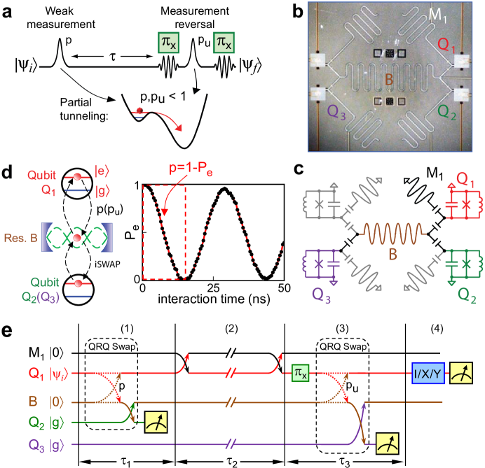
Figure 1: Device geometry and un-collapsing protocol used for QED. a, Quantum un-collapsing protocol in the phase qubit [20, 19]. Top: Pulse sequence, where the weak measurement with strength $p$ is followed by a delay (storage time) $\tau$, and then the measurement reversal, involving a $\pi_{x}$ rotation, a weak measurement with strength $p_{u}$, and a second $\pi_{x}$ rotation. Bottom: The delta-like electrical pulses lower the tunnel barrier for the qubit states on the left of the potential landscape to allow partial tunneling of the $|e\rangle$ state into the well on the right. b-c, Optical micrograph and simplified schematic of the device. Circuit elements are as labeled; those not used in this experiment are in gray. d, Illustration of the qubit-resonator-qubit (QRQ) swap, analogous to the partial tunneling measurement. Left: Schematic for the sequential qubit $Q_{1}$-resonator $B$ swap with swap probability (measurement strength) $p$ ($p_{u}$), followed by a full iSWAP between resonator $B$ and qubit $Q_{2}$ ($Q_{3}$). Right: The on-resonance, unit-amplitude qubit-resonator vacuum Rabi oscillations in the qubit $|e\rangle$ state probability $P_{e}$ (vertical axis), starting with the qubit in $|e\rangle$ and resonator in $|0\rangle$. The measurement strength $p=1-P_{e}$ is set by the interaction time (horizontal axis). e, QED protocol, where we start with $Q_{1}$ in $|\psi_{i}\rangle$, consisting of the following steps: 1. The first weak measurement is performed using the first QRQ swap involving $Q_{1}$-$B$-$Q_{2}$, with strength $p$. $Q_{2}$ is measured immediately, and only null outcomes ($Q_{2}$ in $|g\rangle$) are accepted. 2. The state is swapped from $Q_{1}$ into memory resonator $M_{1}$ and stored for a relatively long time $\tau_{2}$, following which the state is swapped back into $Q_{1}$. 3. The weak measurement reversal is performed using a $\pi_{x}$ rotation on $Q_{1}$ and a second QRQ swap with strength $p_{u}$ to qubit $Q_{3}$. $Q_{3}$ is then measured, and only null outcomes ($Q_{3}$ in $|g\rangle$) are accepted. 4. The double-null outcomes are analyzed using tomography of $Q_{1}$ to evaluate $Q_{1}$’s final density matrix. To save time and reduce errors, we do not perform the final $\pi_{x}$ rotation appearing in the full un-collapsing protocol.

Remarkably, the final no-jump state is identical to $|\psi_{i}\rangle$ if we choose $1-p_{u}=(1-p)e^{-\Gamma\tau}$; the probability of this (desired) outcome is $P_{f}^{nj}=\langle\psi_{f}^{nj}|\psi_{f}^{nj}\rangle=(1-p)e^{-\Gamma\tau}$, while the probability of the undesirable jump outcome $|g\rangle$ is $P_{f}^{j}=\left|\beta\right|^{2}(1-p)^{2}e^{-\Gamma\tau}(1-e^{-\Gamma\tau})$. [24] As the probability $P_{f}^{j}$ falls to zero more quickly than $P_{f}^{nj}$ as $p\rightarrow 1$, increasing the measurement strength $p$ towards 1 results in a high likelihood of recovering the initial state. This comes at the expense of a low probability $P_{\rm{DN}}=P_{f}^{nj}+P_{f}^{j}$ of the double-null result.

Results

The weak measurement in Fig. 1a is performed by partial tunneling. We used partial tunneling for the measurement in QED (see below), but as it consistently yielded low fidelities, we also developed an alternative, more extensive device and protocol, shown in Fig. 1b-d. The device is similar to that in Ref. [25], with three phase qubits, $Q_{1}$, $Q_{2}$, and $Q_{3}$, coupled to a common, half-wavelength coplanar waveguide bus resonator $B$, with a memory resonator $M_{1}$ also coupled to $Q_{1}$. Relevant parameters are tabulated in the Supplementary Information.

The alternative partial measurement method is illustrated in Fig. 1d. Qubit $Q_{1}$ is the target, and $Q_{2}$ and $Q_{3}$ are ancillae, entangled with $Q_{1}$ via the resonator bus $B$, such that a projective measurement of $Q_{2}$ or $Q_{3}$ results in a weak measurement of $Q_{1}$. The entanglement begins with a partial swap between $Q_{1}$ and the resonator $B$: When qubit $Q_{1}$, initially in $|e\rangle$, is tuned to resonator $B$, the probability $P_{e}$ of finding the qubit in $|e\rangle$ oscillates with unit amplitude at the vacuum Rabi frequency [26, 27, 28]. A partial swap with swap probability $p=1-P_{e}$ is achieved by controlling the interaction time, entangling $Q_{1}$ and $B$. We then use a complete swap (an “iSWAP”) between resonator $B$ and qubit $Q_{2}$ ($Q_{3}$), transferring the entanglement, followed by a projective measurement of $Q_{2}$ ($Q_{3}$). In general, we start with $Q_{1}$ in $|\psi_{i}\rangle=\alpha|g\rangle+\beta|e\rangle$ and perform the qubit-resonator-qubit (QRQ) swap, followed by measurement of the ancilla. A null outcome ($Q_{2}$ or $Q_{3}$ in $|g\rangle$) yields the $Q_{1}$ state $\alpha|g\rangle+\beta\sqrt{1-p}|e\rangle$, as with partial tunneling. The swap probability $p$ is therefore equivalent to the measurement strength.

Our QED protocol can protect against energy decay of the quantum state. However, as dephasing in these qubits is an important error source, against which the QED protocol does not protect, we store the intermediate quantum state in the memory resonator $M_{1}$, which does not suffer from dephasing (as indicated by $T_{2}\cong 2T_{1}$ for the resonator; see Supplementary Information).

Our full QED protocol is shown in Fig. 1e, starting with the initial state of the system as

$$|\Psi_{i}\rangle=(\alpha|ggg\rangle+\beta|egg\rangle)\otimes|00\rangle,$$ (2)

where $|q_{1}q_{2}q_{3}\rangle$ represents the state of the qubits $Q_{1}$, $Q_{2}$ and $Q_{3}$, with the ground state $|00\rangle$ of the $B$ and $M_{1}$ resonators listed last. In step 1, we use a QRQ swap between $Q_{1}$, $B$ and $Q_{2}$ with swap probability (measurement strength) $p$, followed immediately by measurement of $Q_{2}$. This step takes a time $\tau_{1}$ of up to 15 ns, depending on $p$. A null outcome ($Q_{2}$ in $|g\rangle$) yields $|\Psi_{1}\rangle=\alpha|ggg\rangle|00\rangle+\beta\sqrt{1-p}\,|egg\rangle|00\rangle$ (a more precise expression appears in the Supplementary Information). In step 2, we swap the quantum state from $Q_{1}$ into $M_{1}$, wait a relatively long time $\tau=\tau_{2}$, during which the state in $M_{1}$ decays at a rate $\Gamma=1/T_{1}$, and we then swap the state back to $Q_{1}$. In the no-jump case, the state becomes $|\Psi_{2}^{nj}\rangle=\alpha|ggg\rangle|00\rangle+\beta\sqrt{1-p}\,e^{-\Gamma\tau_{2}/2}|egg\rangle|00\rangle$. We then perform step 3, comprising a $\pi_{x}$ rotation on $Q_{1}$ followed by the second QRQ swap with strength $p_{u}$, involving $Q_{1}$, $B$ and $Q_{3}$, which takes a time $\tau_{3}$. $\tau_{3}$ is between 20 and 35 ns, depending on $p_{u}$, dominated by the 20 ns-duration $\pi_{x}$ pulse. $Q_{3}$ is then measured, with a null outcome ($Q_{3}$ in $|g\rangle$) corresponding to

$$|\Psi_{f}^{nj}\rangle=(\alpha\sqrt{1-p_{u}}|e\rangle+\beta\sqrt{1-p}\,e^{-\Gamma\tau_{2}/2}|g\rangle)\otimes|gg\rangle|00\rangle.$$ (3)

We recover the initial state $|\Psi_{i}\rangle$ if we set $1-p_{u}=(1-p)e^{-\Gamma\tau_{2}}$, with the undesired jump cases mostly eliminated by the double-null selection. To shorten the sequence, we do not perform the final $\pi_{x}$ rotation, so the amplitudes of $Q_{1}$’s $|g\rangle$ and $|e\rangle$ states are reversed compared to the initial state. In step 4, we apply tomography pulses and then measure $Q_{1}$ to determine its final state, keeping the results that correspond to the double-null outcomes ($Q_{2}$ and $Q_{3}$ in $|g\rangle$).

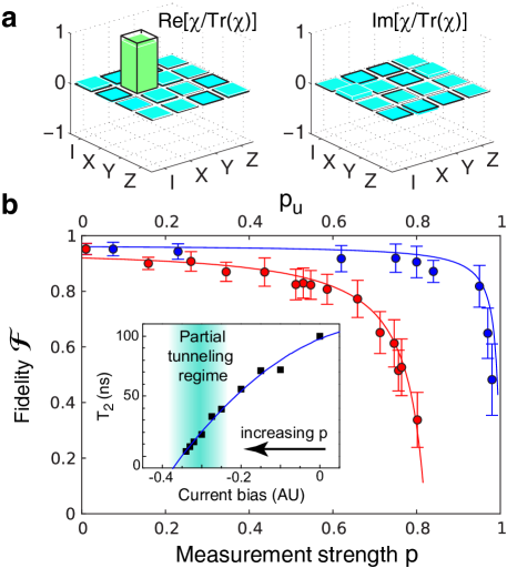
Figure 2: Fidelity of the uncollapsing protocol without storage. a, Measured $\chi/\operatorname{Tr}(\chi)$ (bars with color), where $\chi$ is the non-trace-preserving quantum process tomography matrix for the sequence in Fig. 1e excluding step 2, here with $p=p_{u}=0.75$. The desired matrix, $\chi^{\textrm{ideal}}$, corresponds to a $\pi$ rotation about the Bloch sphere $x$ axis (identified by black frames). b, Process fidelity ${\mathcal{F}}$ for both the three-qubit QRQ-based un-collapsing (blue circles) and the single-qubit partial-tunneling version (red circles) [20], both as a function of $p=p_{u}$. Error bars represent statistical errors extracted from repeated measurements. The process fidelity is above 0.9 for $p\leq 0.8$ using the QRQ swaps, while for the partial tunneling scheme it decreases significantly for $p\geq 0.5$. This decrease is primarily due to reduction in qubit $T_{2}$ with measurement current bias, shown in the inset; partial tunneling occurs in the shaded region. Blue line is a simulation using $\kappa_{1}=\kappa_{3}=0.985$, $\kappa_{2}=1$, and $\kappa_{\varphi}=0.95$ (see Supplementary Information); the red line is a guide to the eye.

We use quantum process tomography to characterize the performance of the protocol, starting with the four initial states $\left\{|g\rangle,|g\rangle-i|e\rangle,|g\rangle+|e\rangle,|e\rangle\right\}$ and measuring the one-qubit process matrix $\chi$. As we reject outcomes where $Q_{2}$ and $Q_{3}$ are not measured in $|g\rangle$, the process is not trace-preserving, so the linear map satisfies $\rho_{f}P_{\rm DN}=\sum_{n,m}\chi_{nm}E_{n}\rho_{i}E^{+}_{m}$, where $\rho_{i}$ and $\rho_{f}$ are the normalized initial and final density matrices of $Q_{1}$, and $E_{n}$ is the standard Pauli basis $\left\{I,X,Y,Z\right\}$. We define the process fidelity ${\mathcal{F}}$ as [29] ${\mathcal{F}}=\operatorname{Tr}(\chi^{\textrm{ideal}}\chi)/\operatorname{Tr}(\chi)$, where $\chi^{\textrm{ideal}}$ corresponds to the desired unitary operation (here given by $\pi_{x}$), and the divisor accounts for post-selection.[30]

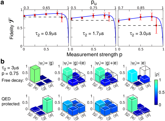
Figure 3: QED-based quantum state protection from energy relaxation. a, Process fidelity ${\mathcal{F}}$ as a function of measurement strength $p$ for the full QED protocol for three storage times $\tau_{2}=0.9,~{}1.7$ and 3 $\mu$s in memory resonator $M_{1}$ ($T_{1}=2.5\mu$s). The un-collapsing swap probability $p_{u}$ is indicated on the top axis (see text). Circles with error bars are measured data; lines are simulations (see Supplementary Information). Horizontal dashed lines in each panel give the free-decay process fidelity; the improvement from QED is most significant for larger $\tau_{2}$. The statistical errors increase with increasing QRQ measurement strength $p$, due to the decrease in sample size (fewer double-null outcomes); we compensate for dynamic phases (see Supplementary Information). b, Final density matrices (bars with color) without (top row) and with (bottom row) QED, with $p=0.75$, for the four initial states as labeled, following a $\tau_{2}=3~{}\mu$s storage time ($e^{-\tau_{2}/T_{1}}=0.3$). The desired error-free density matrices are shown by black frames. We only display the absolute values of the density matrix elements $|\rho|$. Note that the QED-protected final states differ from the initial state by a $\pi$ rotation.

We first tested the process with no storage, entirely omitting step 2 in Fig. 1e, and choosing $p_{u}=p$; we also delayed the measurement of $Q_{2}$ to the end of step 3 to minimize crosstalk (see Methods). Figure 2a shows the measured $\chi/\operatorname{Tr}(\chi)$ for $p=p_{u}=0.75$; the calculated process fidelity is ${\mathcal{F}}=0.92$. In Fig. 2b we show the measured process fidelity ${\mathcal{F}}$ as a function of the QRQ measurement strength $p=p_{u}$ (blue circles).

We can compare our no-storage un-collapsing fidelity to that obtained using partial tunneling for the weak measurement of a single qubit [20], shown in Fig. 2b (red circles). We see that even though the QRQ-based protocol is more complex, it achieves much better fidelities for $p\geq 0.5$. This is mostly because of strong dephasing and two-level state effects [27, 4] during the partial tunneling current pulse (see inset in Fig. 2b).

We then tested the full QRQ protocol’s ability to protect from energy decay. The un-collapsing strength $p_{u}$ is given by [19] $1-p_{u}=(1-p)\kappa_{1}\kappa_{2}/\kappa_{3}$, where $\kappa_{2}=\exp(-\tau_{2}/T_{1})$ and $\kappa_{1}$ and $\kappa_{3}$ are similar energy relaxation factors for the steps 1 and 3 (here $\kappa_{1}\approx\kappa_{3}\approx 0.985$; see Supplementary Information). In Fig. 3a we display the measured fidelities for the storage durations $\tau_{2}=0.9,~{}1.7$ and 3 $\mu$s for the memory resonator with $T_{1}=2.5~{}\mu$s, compared to simulations using the pure dephasing factor $\kappa_{\varphi}=0.95$ (see Ref. [19] and Supplementary Information). The simulations are in excellent agreement with the data, and we see a marked improvement in the storage fidelity using QED over that of free decay (dashed line in each panel).

It is interesting to note that in Fig. 3a, the process fidelity is significantly improved even for zero measurement strength $p=0$ (note that $p_{u}>0$), implying that a simpler QED protocol still provides some protection against energy relaxation.

Another way to test QED is to monitor the evolution of individual quantum states. In Fig. 3b we display the final density matrices measured either without (top row) or with (bottom row) QED, for four initial states in $Q_{1}$, with storage in the memory $M_{1}$ for $\tau_{2}\approx 3~{}\mu$s. Other than for the initial ground state $|g\rangle$, which does not decay, we see that the QED-protected states are much closer to the desired outcomes than the free-decay states (note the $\pi$ rotation). If we look at the off-diagonal terms in the middle panels, they have decayed from 0.5 to about 0.4; this decay takes about 1.1 $\mu$s without QED, so the lifetime is increased by $3~{}\mu{\rm s}/1.1~{}\mu{\rm s}\approx 3$. Also, if we look at Fig. 3a, the free-decay fidelity at 0.9 $\mu$s (left panel) is about the same as the maximum QED fidelity at 3.0 $\mu$s (right panel), also giving a factor of three improvement.

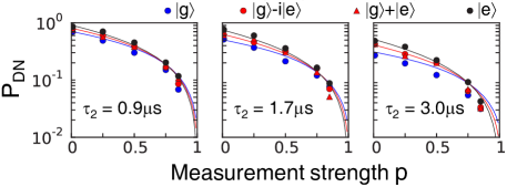
Figure 4: QED selection probability. The QED protocol uses post-selection to reject state decay errors. The probability of accepting an outcome, i.e. the double-null probability $P_{\textrm{DN}}$, falls with measurement strength $p$. Here we display $P_{\textrm{DN}}$ as a function of $p$, corresponding to the data in Fig. 3a, for each value of storage time $\tau_{2}$. Lines are predicted by theory.

The price paid for the lifetime improvement is the small fraction of outcomes accepted by the QED post-selection, shown in Fig. 4. The double-null probability $P_{\rm{DN}}$ decreases with increasing measurement strength $p$ for all initial states. A balance must therefore be struck between a larger $T_{1}$ improvement, occurring for larger $p$, and a larger fraction of accepted outcomes, which occurs for smaller $p$.

In conclusion, we have implemented a practical QED protocol, based on quantum un-collapsing, that suppresses the intrinsic energy relaxation of a quantum state in a superconducting circuit, increasing the effective lifetime by about a factor of three. We note that the phase qubits in our design could be replaced by better-performing qubits [10], on which real-time quantum non-demolition measurement and feedback control are feasible[33, 34, 3]. This could enable sufficient coherence for demonstrating a practical fault-tolerant quantum architecture.

Methods

Readout correction and crosstalk cancellation. All data are corrected for the qubit readout fidelities before further processing. The readout fidelities for $|g\rangle$ ($F_{g}$) and $|e\rangle$ ($F_{e}$) of $Q_{1}$, $Q_{2}$, and $Q_{3}$ are $F_{1g}=0.95$, $F_{1e}=0.89$, $F_{2g}=0.94$, $F_{2e}=0.88$, $F_{3g}=0.94$, $F_{3e}=0.91$, respectively. Crosstalk is another concern when performing QED to protect quantum states. We read out $Q_{2}$ immediately after the first QRQ swap in step 1 in Fig. 1e to avoid decay in $Q_{2}$. However, due to measurement crosstalk in the qubit circuit, this measurement can result in excitations in resonator $B$; while this does not directly affect the other qubits, we must reset the resonator prior to the second QRQ swap. This is done during the storage in the memory resonator, by performing a swap between $B$ and $Q_{3}$, and then using a spurious two-level defect coupled to $Q_{3}$ to erase the excitation in $Q_{3}$. As the storage time in $M_{1}$ is several microseonds, there is sufficient time to reset both $B$ and $Q_{3}$ prior to the second QRQ swap.

The intermediate reset of $B$ could not be performed when doing the experiments in Fig. 2, for which there is no storage interval. To avoid crosstalk in those measurements, we postponed the measurement of $Q_{2}$ until the end of the second QRQ sequence, to step 3 of Fig. 1e. The $|e\rangle$ state probability in $Q_{2}$ drops by about 6% during this delay time, as estimated from $Q_{2}$’s $T_{1}$. We have corrected for this drop when evaluating the $Q_{2}$ measurements for Fig.2.

Acknowledgments
This work was supported by the National Basic Research Program of China (2012CB927404), the National Natural Science Foundation of China (11222437, 11174248, and J1210046), Zhejiang Provincial Natural Science Foundation of China (LR12A04001), and IARPA/ARO grant W911NF-10-1-0334 of USA. H.W. acknowledges supports by Program for New Century Excellent Talents in University (NCET-11-0456) and by Synergetic Innovation Center of Quantum Information and Quantum Physics. Devices were made at the UC Santa Barbara Nanofabrication Facility, a part of the NSF funded National Nanotechnology Infrastructure Network.

Author contributions
Y.P.Z., A.N.K., H.W. designed and analyzed the experiment carried out by Y.P.Z. All authors contributed to the experimental set-up and helped to write the paper.

Supplementary Information

I Qubit and resonator parameters used in experiment

The qubits and resonators used in this experiment were all produced in a multi-layer lithographic process on single-crystal sapphire substrates. The qubits are phase qubits, each consisting of a $2\,\mu\mathrm{m}^{2}$ Al/AlO_x/Al junction in parallel with a $1$ pF Al/a-Si:H/Al shunt capacitor and a 720 pH loop inductance (design values). The resonators are single-layer aluminum coplanar waveguide resonators. We use interdigitated coupling capacitors between the qubits and the resonators. Standard performance parameters of individual elements are listed in Table S1.

	freq.		$T_{1}$		$T_{2}$		$T_{SE}$		coupling strength
	(GHz)		(ns)		(ns)		(ns)		(MHz)
$Q_{1}$	6.01		580		140		500		34.7 ($\leftrightarrow B$)
$Q_{2}$	5.90		614		100		510		34.1 ($\leftrightarrow B$)
$Q_{3}$	5.81		580		150		430		33.3 ($\leftrightarrow B$)
$B$	6.24		3000		$\sim$5000		$\ast$
$M_{1}$	7.55		2500		$\sim$5000		$\ast$		56.8 ($\leftrightarrow Q_{1}$)

Table S1: Operating characteristics for qubits $Q_{1}$, $Q_{2}$, $Q_{3}$, the bus resonator $B$, and the memory resonator $M_{1}$. We show the $|g\rangle-|e\rangle$ splitting frequency for the qubits, the resonance frequency for the resonators, as well as each element’s measured energy relaxation time $T_{1}$, Ramsey dephasing time $T_{2}$, and spin-echo dephasing time $T_{SE}$. Qubit lifetimes are at the listed frequencies, and resonator lifetimes are measured using photon swaps with a qubit; the coupling strengths are from vacuum Rabi oscillations. [26, 25, 27]

II State evolution during the QRQ-based quantum error detection protocol

In this section we discuss the state evolution in the actual experimental protocol, based on the QRQ swaps. We include the dynamic phases in the analysis but for simplicity neglect imperfections as well as decoherence in the unitary operations, while including energy relaxation during the state storage in the memory resonator (step 2 in Fig. 1e of the main text).

Assuming no errors in the preparation of the target qubit $Q_{1}$, the initial state of the system prior to step 1 shown in Fig. 1e is [see Eq. (2) in the main text]

$$|\Psi_{i}\rangle=\alpha|ggg\rangle|00\rangle+\beta|egg\rangle|00\rangle=(\alpha|g\rangle+\beta|e\rangle)\otimes|gg\rangle|00\rangle,$$ (S1)

where $|\alpha|^{2}+|\beta|^{2}=1$ and the notation $|q_{1}\,q_{2}\,q_{3}\rangle\,|b\,m_{1}\rangle$ displays the quantum states of the qubits $Q_{1}$, $Q_{2}$, and $Q_{3}$, as well as the states of the bus $B$ and memory $M_{1}$ resonators; the notation including the outer product sign “$\otimes$” uses the same order for the system elements.

Step 1 of the procedure (Fig. 1e) is equivalent to the first partial measurement of the qubit $Q_{1}$ in Fig. 1a with strength $p$. This step consists of the QRQ swap $Q_{1}$–$B$–$Q_{2}$, followed by measurement of qubit $Q_{2}$. First, the partial swap between the qubit $Q_{1}$ and bus $B$ with the swap probability $p$ results in the state

$$|\Psi_{1a}\rangle=\alpha|ggg\rangle|00\rangle+\beta e^{i\theta_{p}}(\sqrt{1-p}\,|egg\rangle|00\rangle-ie^{i\tilde{\theta}_{p}}\sqrt{p}\,|ggg\rangle|10\rangle),$$ (S2)

where $\theta_{p}$ and $\tilde{\theta}_{p}$ are the dynamic phases accumulated when the frequency of qubit $Q_{1}$ is tuned into and out of resonance with the resonator $B$ [each term in Eq. (S2) assumes a separate rotating frame]. The factor $-i$ in the last term comes from the ideal qubit-resonator evolution described by the standard Hamiltonian. After this partial swap, the resonator $B$ is no longer in the ground state. The second part of the QRQ swap fully transfers the excitation from $B$ into $Q_{2}$, resulting in the state

$$|\Psi_{1b}\rangle=\alpha|ggg\rangle|00\rangle+\beta e^{i\theta_{p}}(\sqrt{1-p}\,|egg\rangle|00\rangle-\sqrt{p}\,e^{i\theta_{pa}}|geg\rangle|00\rangle),$$ (S3)

where the phase $\theta_{pa}$ combines $\tilde{\theta}_{p}$ and the dynamic phase accumulated during the full swap. The minus sign in the last term is due to the additional factor $-i$, appearing when the excitation in the resonator $B$ swaps to $Q_{2}$ (this is why the full swap is termed an “iSWAP”).

After the QRQ swap $Q_{1}$–$B$–$Q_{2}$, the qubit $Q_{2}$ is measured projectively (“strongly”) and only the outcome $|g\rangle$ is selected. Phase qubits are measured [26] by lowering the tunnel barrier between the right and left potential wells shown in the bottom panel of Fig. 1a, with a high likelihood of tunneling to the right well if the qubit is in the excited state $|e\rangle$, while there is a very small tunneling probability if the qubit is in its ground state $|g\rangle$. When a qubit that is initially in a superposition of $|g\rangle$ and $|e\rangle$ tunnels to the right well, the subsequent rapid energy decay in the right well destroys any coherence between $|g\rangle$ and $|e\rangle$ states. The barrier is lowered only for a few nanoseconds, and the quantum state projection occurs during this time. Actual readout of the measurement result takes place many microseconds later, using a SQUID flux measurement.

In the case of the measurement result $|g\rangle$ (no tunneling for qubit $Q_{2}$), the system state (S3) collapses to the state

$$|\Psi_{1c}\rangle=\alpha|ggg\rangle|00\rangle+\beta e^{i\theta_{p}}\sqrt{1-p}\,|egg\rangle|00\rangle.$$ (S4)

Notice that while the state (S3) is normalized, $\langle\Psi_{1b}|\Psi_{1b}\rangle=1$, the post-selected state (S4) is not normalized, so that $\langle\Psi_{1c}|\Psi_{1c}\rangle$ is the probability of the $|g\rangle$ outcome, while the normalized state would be $|\Psi_{1c}\rangle/\sqrt{\langle\Psi_{1c}|\Psi_{1c}\rangle}$. We prefer here to use unnormalized states as in Eq. (S4) because these are linearly related to the initial state, in contrast to the normalized states. The state (S4) can be written as $|\Psi_{1c}\rangle=(\alpha|g\rangle+\beta e^{i\theta_{p}}\sqrt{1-p}\,|e\rangle)\,|gg\rangle|00\rangle$, so at the end of this step we essentially have a one-qubit state in $Q_{1}$, even though other elements of the system are entangled with $Q_{1}$ during the evolution of this step.

Step 2 of the protocol (Fig. 1e) involves storing $Q_{1}$’s state in the memory resonator $M_{1}$ for a relatively long time $\tau_{2}$, which corresponds to the delay $\tau$ in the protocol in Fig. 1a in the main text. We first perform an iSWAP between $Q_{1}$ and $M_{1}$, resulting in the state

$$|\Psi_{2a}\rangle=\alpha|ggg\rangle|00\rangle-i\beta e^{i\theta_{p}}e^{i\tilde{\theta}_{s}}\sqrt{1-p}\,|ggg\rangle|01\rangle,$$ (S5)

where $\tilde{\theta}_{s}$ is the dynamic phase accumulated when tuning $Q_{1}$ into the resonance with $M_{1}$. With $Q_{1}$ now in its ground state, we detune $Q_{1}$ from $M_{1}$ to its “idle” frequency, and wait a time $\tau_{2}$. During this time the state in the resonator $M_{1}$ decays in energy at the rate $\Gamma=1/T_{1}$, where $T_{1}=2.5\,\mu$s is the energy relaxation time of $M_{1}$, so that the overall decay factor is $\kappa_{2}=e^{-\Gamma\tau_{2}}$ (pure dephasing is negligible).

The decay in $M_{1}$ can be treated by considering two scenarios: [19] either the state of $M_{1}$ “jumps” to $|g\rangle$ during the storage time $\tau_{2}$ or there is no jump. In the jump scenario the resulting unnormalized state is

$$|\Psi_{2b}^{j}\rangle=\beta\sqrt{1-p}\,\sqrt{1-e^{-\Gamma\tau_{2}}}\,|ggg\rangle|00\rangle,$$ (S6)

where the overall phase is not important. We will return to this scenario later, focusing first on the no-jump scenario, which produces the unnormalized state

$$|\Psi_{2b}^{nj}\rangle=\alpha|ggg\rangle|00\rangle-i\beta e^{i\theta_{p}}e^{i\tilde{\theta}_{s}}\sqrt{1-p}\,e^{-\Gamma\tau_{2}/2}|ggg\rangle|01\rangle.$$ (S7)

After the storage time $\tau_{2}$ we swap the state in $M_{1}$ back to $Q_{1}$, so that at the end of step 2 the no-jump state becomes

$$|\Psi_{2c}^{nj}\rangle=\alpha|ggg\rangle|00\rangle+\beta e^{i(\theta_{p}+\theta_{s})}\sqrt{1-p}\,e^{-\Gamma\tau_{2}/2}|egg\rangle|00\rangle,$$ (S8)

where the phase $\theta_{s}$ includes $\tilde{\theta}_{s}$ [see Eq. (S5)], the similar dynamic phase accumulated during the swap back to $Q_{1}$, the $\pi$-shift due to the factor $(-i)^{2}$, and the phase $2\pi\Delta f\tau_{2}$ accumulated due to the frequency difference $\Delta f$ between the resonator $M_{1}$ and the qubit $Q_{1}$ at its “idle” frequency. After the step is completed, we again have essentially a one-qubit state.

Step 3 of the protocol consists of a $\pi_{x}$ rotation, the second QRQ swap $Q_{1}$–$B$–$Q_{3}$ with strength $p_{u}$, and the projective measurement of $Q_{3}$ (this step is analogous to the second partial measurement in Fig. 1a). The $\pi_{x}$ rotation applied to $Q_{1}$ exchanges the amplitudes of its $|g\rangle$ and $|e\rangle$ states in Eq. (S8):

$$|\Psi_{3a}^{nj}\rangle=\alpha|egg\rangle|00\rangle+\beta e^{i(\theta_{p}+\theta_{s})}\sqrt{1-p}\,e^{-\Gamma\tau_{2}/2}|ggg\rangle|00\rangle.$$ (S9)

The partial swap between $Q_{1}$ and $B$ then yields the state

$$|\Psi_{3b}^{nj}\rangle=\alpha e^{i\theta_{u}}(\sqrt{1-p_{u}}\,|egg\rangle|00\rangle-ie^{i\tilde{\theta}_{u}}\sqrt{p_{u}}\,|ggg\rangle|10\rangle)\hskip 34.14322pt$$

$$\hskip 34.14322pt+\beta e^{i(\theta_{p}+\theta_{s})}\sqrt{1-p}\,e^{-\Gamma\tau_{2}/2}|ggg\rangle|00\rangle,$$ (S10)

where $\theta_{u}$ and $\tilde{\theta}_{u}$ are the dynamic phases accumulated during this partial swap. Next, the QRQ swap is completed with a full iSWAP between $B$ and $Q_{3}$, yielding the state

$$|\Psi_{3c}^{nj}\rangle=[(e^{i\theta_{u}}\alpha\sqrt{1-p_{u}}\,|egg\rangle+e^{i(\theta_{p}+\theta_{s})}\beta\sqrt{1-p}\,e^{-\Gamma\tau_{2}/2}|ggg\rangle)$$

$$\hskip 34.14322pt-e^{i(\theta_{u}+\theta_{ua})}\alpha\sqrt{p_{u}}\,|gge\rangle]\otimes|00\rangle,$$ (S11)

where $\theta_{ua}$ combines $\tilde{\theta}_{u}$ and the dynamic phase accumulated during the last iSWAP. Finally, the measurement of $Q_{3}$ and the selection of the result $|g\rangle$ (thus corresponding to an overall double-null outcome) produces the no-jump state

$$|\Psi_{f}^{nj}\rangle=(\alpha\sqrt{1-p_{u}}\,|e\rangle+e^{i(\theta_{p}+\theta_{s}-\theta_{u})}\beta\sqrt{1-p}\,e^{-\Gamma\tau_{2}/2}|g\rangle)\otimes|gg\rangle|00\rangle,$$ (S12)

where we ignore the unimportant overall phase.

Equation (S12) coincides with Eq. (3) of the main text, if we neglect the dynamic phase $\theta_{p}+\theta_{s}-\theta_{u}$. This phase does not depend on the initial state, but in general depends on $p$, $p_{u}$, and $\tau_{2}$. To restore the initial qubit state (up to a $\pi_{x}$ rotation), this phase can be corrected by an additional single-qubit phase gate (rotation about the $z$ axis of the Bloch sphere). In the experiment we typically did not perform this correction, and instead compensated for this phase numerically in the quantum process tomography analysis. However, we have checked explicitly that for the initial states $\ket{g}-i\ket{e}$ and $\ket{g}+\ket{e}$ (using the same QED protocol parameters), the measured output states differ by a phase of $\pi/2$, as expected.

Note that we completely omit step 2 when testing the protocol with no storage in $M_{1}$, i.e. with $\tau_{2}=0$ (see Fig. 2 of the main text). In this case there is no dynamic phase $\theta_{s}$ in Eq. (S12), we have no delay-based decay so that $e^{-\Gamma\tau_{2}/2}=1$, and also the dynamic phases $\theta_{p}$ and $\theta_{u}$ cancel each other because $p_{u}=p$ and therefore $\theta_{u}=\theta_{p}$. In reality there is still a small amount of energy decay occurring in steps 1 and 3. We take this into account in the numerical simulations as described in the next section.

Now let us return to the scenario when the energy relaxation event (the jump) occurs during step 2, producing the state $|\Psi_{2b}^{j}\rangle$ given by Eq. (S6). After performing the swap between the memory resonator and $Q_{1}$, this state remains the same, $|\Psi_{2c}^{j}\rangle=|\Psi_{2b}^{j}\rangle$, because all elements are in their ground states. In step 3 of the protocol, following the $\pi_{x}$ pulse, the state becomes

$$|\Psi_{3a}^{j}\rangle=\beta\sqrt{1-p}\,\sqrt{1-e^{-\Gamma\tau_{2}}}\,|egg\rangle|00\rangle,$$ (S13)

and following the partial swap between $Q_{1}$ and $B$ this state evolves into

$$|\Psi_{3b}^{j}\rangle=\beta\sqrt{1-p}\,\sqrt{1-e^{-\Gamma\tau_{2}}}\,(\sqrt{1-p_{u}}\,|egg\rangle|00\rangle-ie^{i\tilde{\theta}_{u}}\sqrt{p_{u}}\,|ggg\rangle|10\rangle)$$ (S14)

(the overall phase $\theta_{u}$ is now unimportant), and after the full iSWAP between $B$ and $Q_{3}$ it becomes

$$|\Psi_{3c}^{j}\rangle=\beta\sqrt{1-p}\,\sqrt{1-e^{-\Gamma\tau_{2}}}\,(\sqrt{1-p_{u}}\,|egg\rangle-e^{i\theta_{ua}}\sqrt{p_{u}}\,|gge\rangle)\otimes|00\rangle.$$ (S15)

After the measurement of $Q_{3}$ and selection of the null result $|g\rangle$, the final state in the jump scenario is

$$|\Psi_{f}^{j}\rangle=\beta\sqrt{1-p}\,\sqrt{1-e^{-\Gamma\tau_{2}}}\,\sqrt{1-p_{u}}\,|e\rangle\otimes|gg\rangle|00\rangle,$$ (S16)

so that the qubit $Q_{1}$ is now in the $|e\rangle$ state.

The squared norm of the no-jump final state $|\Psi_{f}^{nj}\rangle$ in Eq. (S12) is the probability of the no-jump scenario (which includes the double-null outcome selection),

$$P^{nj}_{f}\equiv\langle\Psi_{f}^{nj}|\Psi_{f}^{nj}\rangle=|\alpha|^{2}(1-p_{u})+|\beta|^{2}(1-p)e^{-\Gamma\tau_{2}}.$$ (S17)

Notice that this probability becomes $P^{nj}_{f}=(1-p)e^{-\Gamma\tau_{2}}$ if we choose $1-p_{u}=(1-p)e^{-\Gamma\tau_{2}}$. The squared norm of the state $|\Psi_{f}^{j}\rangle$ in Eq. (S16) is the probability of the jump scenario,

$$P^{j}_{f}\equiv\langle\Psi_{f}^{j}|\Psi_{f}^{j}\rangle=|\beta|^{2}(1-p)(1-p_{u})(1-e^{-\Gamma\tau_{2}}).$$ (S18)

This probability is given by $P_{f}^{j}=|\beta|^{2}(1-p)^{2}e^{-\Gamma\tau_{2}}(1-e^{-\Gamma\tau_{2}})$ if we choose $1-p_{u}=(1-p)e^{-\Gamma\tau_{2}}$. The probabilities $P_{f}^{nj}$ and $P_{f}^{j}$ cover all possible double-null outcomes in this model, so their sum

$$P_{DN}=P_{f}^{nj}+P_{f}^{j}$$ (S19)

is the probability of the double-null outcome.

Combining the two scenarios, the normalized density matrix of the system after the selection of the double-null outcome is

$$\rho_{f}=\frac{|\Psi_{f}^{nj}\rangle\langle\Psi_{f}^{nj}|+|\Psi_{f}^{j}\rangle\langle\Psi_{f}^{j}|}{P_{DN}}.$$ (S20)

In this double-null outcome, note that the target qubit $Q_{1}$ is now unentangled with the other elements, which are all in their ground states. Comparing the resulting state of the qubit $Q_{1}$ with the corresponding final state in the single-qubit protocol based on partial tunneling [see Fig. 1a and Eq. (1) in the main text], we see only two differences: the non-zero dynamic phase $\theta_{p}+\theta_{s}-\theta_{u}$ in Eq. (S12), and the exchange of the amplitudes of the states $|g\rangle$ and $|e\rangle$ due to the absence of the final $\pi_{x}$ pulse. Therefore, our experimental protocol shown in Fig. 1e essentially realizes the un-collapsing protocol shown in Fig. 1a, but with much better experimental fidelity.

III Numerical simulations

For numerical simulations we follow the theory of Ref. [19] and describe decoherence by the energy relaxation factors $\kappa_{1}$, $\kappa_{2}$, and $\kappa_{3}$ (each factor for the corresponding step of the protocol shown in Fig. 1e) and by the factor $\kappa_{\varphi}$, which accounts for pure dephasing during the whole procedure. The primary decay factor is $\kappa_{2}\approx\exp(-\tau_{2}/T_{1})$, where $\tau_{2}=\tau$ is the storage time and $T_{1}=2.5\,\mu$s is the energy relaxation time of the memory resonator. Similarly, $\kappa_{1}$ describes energy relaxation before the first partial measurement and $\kappa_{3}$ describes energy relaxation in between the $\pi_{x}$ pulse and the second partial measurement. Therefore $\kappa_{1}=\exp(-\tilde{\tau}_{1}/T_{1}^{(1)})$ and $\kappa_{3}=\exp(-\tilde{\tau}_{3}/T_{1}^{(3)})$, where $\tilde{\tau}_{1}$ is the effective duration of step 1 in Fig. 1e before the quantum information is partially swaped into the bus resonator, $\tilde{\tau}_{3}$ is the effective duration of step 3 between the $\pi_{x}$ pulse and partial swap into the bus resonator, and $T_{1}^{(1)}$ and $T_{1}^{(3)}$ are the effective energy relaxation times for these steps (mostly determined by the phase qubit $Q_{1}$). We estimate that $\kappa_{1}\approx\kappa_{3}\approx 0.985$, consistent with the energy relaxation time $T_{1}\simeq 0.6\ \mu$s of the phase qubit $Q_{1}$ (see Table S1) and the time $\sim 10$ ns, which the quantum state spends in the phase qubit before the first partial swap (in step 1) and between the $\pi_{x}$ pulse and the second partial swap (in step 3).

The overall pure dephasing factor is $\kappa_{\varphi}=\exp[-\tau_{1}/T_{\varphi}^{(1)}-\tau_{2}/T_{\varphi}^{(2)}-\tau_{3}/T_{\varphi}^{(3)}]$, where $T_{\varphi}^{(i)}$ is the effective pure dephasing time during $i$th step ($1/T_{\varphi}=1/T_{2}-1/2T_{1}$). In simulations we used the value $\kappa_{\varphi}=0.95$, which fits well with the experimental results and is consistent with the qubit parameters in Table S1. Notice that $T_{\varphi}^{(2)}$ is very long since during step 2, the quantum state is stored in the memory resonator, and therefore $\kappa_{\varphi}$ does not depend on $\tau_{2}$. Also notice that because of the $\pi_{x}$ pulse in the procedure (see Fig. 1e), pure dephasing is reduced, essentially due to a spin-echo effect. In the theory we neglect imperfections of the unitary gates and the qubit decoherence after the second partial swap; we also do not accurately consider decoherence processes in the actual multi-component device, essentially reducing it to the single-qubit model of Ref. [19]. In a practical sense, however, these additional imperfections are somewhat accounted for by small adjustments of the parameters $\kappa_{1}$, $\kappa_{3}$, and $\kappa_{\varphi}$. We have checked numerically that slight variations of the parameters $\kappa_{1}$, $\kappa_{3}$, and $\kappa_{\varphi}$ do not affect the simulation results significantly; $\kappa_{3}$ is the most important parameter, and varying its value in the experimentally-expected range of $0.985\pm 0.005$ gives good agreement with the data shown in Fig. 3a of the main text.

In the experiment we do not perform the final $\pi_{x}$ rotation to save time, so in the final state the amplitudes of the states $\ket{g}$ and $\ket{e}$ are exchanged in comparison with the initial state $|\psi_{i}\rangle=\alpha\ket{g}+\beta\ket{e}$ in $Q_{1}$ (here and below we use a lowercase $|\psi\rangle$ to represent the state of $Q_{1}$, in contrast to $|\Psi\rangle$ which represents the state of the complete system of 3 qubits and 2 resonators). Following the approach of Ref. [19], neglecting the dynamic phases, and for the moment neglecting pure dephasing, we can represent the state of the qubit $Q_{1}$ after the double-null outcome selection as an incoherent mixture of the three states $|g\rangle$, $|e\rangle$, and

$$|\psi_{f}^{nj}\rangle=\beta\sqrt{\kappa_{1}\kappa_{2}(1-p)}\ket{g}+\alpha\sqrt{\kappa_{3}(1-p_{u})}\ket{e}.$$ (S21)

The unnormalized state $|\psi_{f}^{nj}\rangle$ occurs in the “no jump” scenario during steps 1, 2, and 3. The squared norm of this wavefunction is the probability of the no-jump scenario,

$$P_{f}^{nj}=\langle\psi_{f}^{nj}|\psi_{f}^{nj}\rangle=\left|\alpha\right|^{2}\kappa_{3}(1-p_{u})+\left|\beta\right|^{2}\kappa_{1}\kappa_{2}(1-p),$$ (S22)

which includes the probability of the double-null outcome selection.

The final state $|g\rangle$ is realized if there was a “jump” to $|g\rangle$ after the $\pi_{x}$ pulse in step 3 and there was zero or one jump during steps 1 and 2. This occurs with the probability

$$P_{f}^{\ket{g}}=(1-\kappa_{3})\left|\alpha\right|^{2}+(1-\kappa_{3})\left|\beta\right|^{2}[(1-\kappa_{1})+\kappa_{1}(1-p)(1-\kappa_{2})],$$ (S23)

which can be easily understood in the classical way (for a qubit starting either in the state $|g\rangle$ or $|e\rangle$). The final state $|e\rangle$ is realized if there was a jump either during step 1 or 2 and no jump during step 3; this occurs with probability

$$P_{f}^{\ket{e}}=\left|\beta\right|^{2}[(1-\kappa_{1})+\kappa_{1}(1-p)(1-\kappa_{2})]\kappa_{3}(1-p_{u}).$$ (S24)

Combining these three scenarios, we obtain the normalized density matrix of the qubit final state:

$$\rho_{f}=\frac{|\psi_{f}^{nj}\rangle\langle\psi_{f}^{nj}|+P_{f}^{\ket{g}}|g\rangle\langle g|+P_{f}^{\ket{e}}|e\rangle\langle e|}{P_{DN}},\,\,\,\,\,$$ (S25)

where

$$P_{DN}=P_{f}^{nj}+P_{f}^{\ket{g}}+P_{f}^{\ket{e}}$$ (S26)

is the probability of the double-null outcome. Notice that there is no factor $P_{f}^{nj}$ in the numerator of Eq. (S25) because it was included in the definition of the unnormalized state $|\psi_{f}^{nj}\rangle$ in Eq. (S21). The unnormalized final density matrix $P_{DN}\rho_{f}$ [the numerator in Eq. (S25)] is linearly related to the initial density matrix $\rho_{i}=|\psi_{i}\rangle\langle\psi_{i}|$, so the linear map used in the analysis of the quantum process tomography is $\rho_{i}\rightarrow P_{DN}\rho_{f}$.

Pure dephasing (described by $\kappa_{\varphi}$) does not affect the probabilities and does not affect the final states $|g\rangle$ and $|e\rangle$. The only effect of pure dephasing is that the off-diagonal matrix elements of $|\psi_{f}^{nj}\rangle\langle\psi_{f}^{nj}|$ are multiplied by $\kappa_{\varphi}$. This is equivalent to multiplying the off-diagonal matrix elements of $\rho_{f}$ given by Eq. (S25) by $\kappa_{\varphi}$. In other words, pure dephasing can be thought of as occurring after (or before) the procedure described by Eq. (S25).

The dynamic phases appearing in the actual experimental procedure affect only the relative phase between the two terms in Eq. (S21). Therefore, the dynamic phases can be taken into account by using a single parameter: the phase shift of the off-diagonal element of the final density matrix. This dynamic phase shift depends on the parameters of the experimental protocol, including the strength $p$ and $p_{u}$ of the two partial measurements (partial swaps) and the storage duration $\tau_{2}$.

IV Analysis of the QED process fidelity

In the main text we use the definition [29]

$${\mathcal{F}}=\frac{\operatorname{Tr}(\chi^{\textrm{ideal}}\chi)}{\operatorname{Tr}(\chi)},$$ (S27)

for the process fidelity of a non-trace-preserving quantum operation. This definition implies that $\chi/\operatorname{Tr}(\chi)$ is the effective process matrix (which is shown e.g. in Fig. 2a of the main text). Notice that $\chi/\operatorname{Tr}(\chi)$ does not correspond to any physical trace-preserving process; however, this is a positive Hermitian matrix with unit trace, and therefore $0\leq{\mathcal{F}}\leq 1$ when $\chi^{\textrm{ideal}}$ corresponds to a unitary operation. The perfect fidelity, ${\mathcal{F}}=1$, requires $\chi=P_{\rm s}\chi^{\textrm{ideal}}$ with $P_{\rm s}\leq 1$ being the selection probability (in this case $P_{\rm s}$ should not depend on the initial state). This justifies the definition (S27).

However, Eq. (S27) is not the only possible definition for the fidelity of a non-trace-preserving quantum process. For example, another natural definition [19] is the averaged state fidelity,

$${\mathcal{F}}_{\rm av}=\frac{\int\operatorname{Tr}(\rho_{f}\rho^{\rm{ideal}}_{f})\,d|\psi_{i}\rangle}{\int d|\psi_{i}\rangle},$$ (S28)

where $\rho_{f}^{\rm ideal}=U|\psi_{i}\rangle\langle\psi_{i}|U^{\dagger}$, $U$ is the desired unitary operation, $\rho_{f}$ is the actual normalized density matrix, and the integration is over all pure initial states $|\psi_{i}\rangle$ with uniform weight (using the Haar measure); in the one-qubit case this is the uniform averaging over the Bloch sphere. Another natural definition is the averaged state fidelity, which is averaged with a weight proportional to the selection probability $P_{\rm s}$ (denoted $P_{\rm DN}$ in the main text),

$${\mathcal{F}}^{\prime}_{\rm av}=\frac{\int\operatorname{Tr}(\rho_{f}\rho^{\rm{ideal}}_{f})P_{\rm s}(|\psi_{i}\rangle)\,d|\psi_{i}\rangle}{\int P_{\rm s}(|\psi_{i}\rangle)\,d|\psi_{i}\rangle}.$$ (S29)

Notice that both ${\mathcal{F}}_{\rm av}$ and ${\mathcal{F}}^{\prime}_{\rm av}$ can be easily calculated when the process matrix $\chi$ is known.

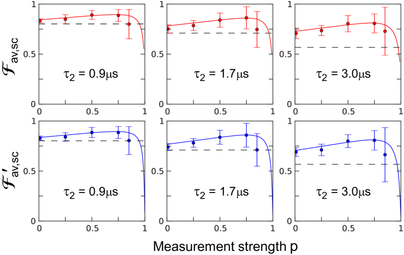
Figure S1: QED process fidelity characterized using different methods. For the same experimental data as in Fig. 3a of the main text, here we show the QED process fidelities calculated via the averaged state fidelities ${\mathcal{F}}_{\rm av}$ and ${\mathcal{F}}_{\rm av}^{\prime}$ defined in Eqs. (S28) and (S29). For easier comparison with Fig. 3a we show the scaled results ${\mathcal{F}}_{\rm av,sc}=(3{\mathcal{F}}_{\rm av}-1)/2$ (top panels) and ${\mathcal{F}}_{\rm av,sc}^{\prime}=(3{\mathcal{F}}_{\rm av}^{\prime}-1)/2$ (bottom panels). As in Fig. 3a, the quantum state is stored for the durations $\tau_{2}=0.9,~{}1.7$, and 3 $\mu$s in the memory resonator $M_{1}$, which has the energy relaxation time $T_{1}=2.5\,\mu$s. The measurement strength (swap probability) $p$ is indicated on the horizontal axis, and the uncollapsing swap probability $p_{u}$ is adjusted as described in the main text. Circles with error bars are the experimental results; lines are simulations. Horizontal dashed lines in each panel show the free-decay process fidelity. The statistical errors increase with increasing measurement strength $p$ due to the decrease in sample size (fewer double-null outcomes). It is seen that all definitions of the QED process fidelity give similar results, and all of them show significant increase of the storage fidelity compared with the case of natural energy relaxation.

For a trace-preserving quantum operation ${\mathcal{F}}^{\prime}_{\rm av}={\mathcal{F}}_{\rm av}$ because $P_{\rm s}=1$, and there is a direct relation [32] $\operatorname{Tr}(\chi^{\textrm{ideal}}\chi)=[(d+1){\mathcal{F}}_{\rm av}-1]/d$, where $d$ is the dimension of the Hilbert space ($d=2$ in our one-qubit case). It is possible to show that in the general non-trace-preserving case the same relation remains valid between ${\mathcal{F}}$ defined by Eq. (S27) and ${\mathcal{F}}_{\rm av}^{\prime}$ defined by Eq. (S29),

$${\mathcal{F}}=\frac{(d+1)\,{\mathcal{F}}_{\rm av}^{\prime}-1}{d}.$$ (S30)

Notice that the denominator ${\operatorname{Tr}(\chi)}$ in Eq. (S27) is equal to the averaged selection probability,

$${\operatorname{Tr}(\chi)}=\frac{\int P_{\rm s}(|\psi_{i}\rangle)\,d|\psi_{i}\rangle}{\int d|\psi_{i}\rangle}.$$ (S31)

We have numerically calculated the process fidelity in our un-collapsing QED experiment using all three definitions (S27)–(S29). For easier comparison with the results for ${\mathcal{F}}$ shown in Fig. 3a of the main text, in Fig. S1 we scale ${\mathcal{F}}_{\rm av}$ and ${\mathcal{F}}_{\rm av}^{\prime}$ as in Eq. (S30): ${\mathcal{F}}_{\rm av,sc}=(3{\mathcal{F}}_{\rm av}-1)/2$, ${\mathcal{F}}_{\rm av,sc}^{\prime}=(3{\mathcal{F}}_{\rm av}^{\prime}-1)/2$. Notice that for the experimental results ${\mathcal{F}}_{\rm av,sc}^{\prime}$ and ${\mathcal{F}}$ are not exactly equal to each other [in spite of Eq. (S30)] because slightly different algorithms were used in the numerical processing of the over-complete experimental data set. Comparing Fig. S1 with Fig. 3a, we see that the experimental results using the three fidelity definitions are close to each other, and all of them show significant increase of the fidelity due to the un-collapsing-based QED procedure.

References

- [1] You, J. and Nori, F. Superconducting circuits and quantum information. Physics Today 58, 42 (2005).
- [2] Clarke, J. and Wilhelm, F. K. Superconducting quantum bits. Nature 453, 1031-1042 (2008).
- [3] Devoret, M. H. and Schoelkopf, R. J. Superconducting circuits for quantum information: an outlook. Science 339, 1169 (2013).
- [4] Sun, G. et al. Tunable quantum beam splitters for coherent manipulation of a solid-state tripartite qubit system. Nature Commun. 1, 51 (2010).
- [5] Niskanen A. O. et al. Quantum Coherent Tunable Coupling of Superconducting Qubits. Science 316, 723 (2011).
- [6] Mariantoni, M. et al. Implementing the Quantum von Neumann Architecture with Superconducting Circuits. Science 334, 61 (2011).
- [7] Abdumalikov Jr, A. A. et al. Experimental realization of non-Abelian non-adiabatic geometric gates. Nature 496, 482-485 (2013).
- [8] Paik, H. et al. Observation of High Coherence in Josephson Junction Qubits Measured in a Three-Dimensional Circuit QED Architecture. Phys. Rev. Lett. 107, 240501 (2011).
- [9] Rigetti, C. et al. Superconducting qubit in a waveguide cavity with a coherence time approaching 0.1 ms. Phys. Rev. B 86, 100506 (2012).
- [10] Barends, R. et al. Coherent Josephson qubit suitable for scalable quantum integrated circuits. Phys. Rev. Lett. 111, 080502 (2013).
- [11] Bylander, J. et al. Noise spectroscopy through dynamical decoupling with a superconducting flux qubit. Nature Phys. 7, 565-570 (2011).
- [12] Reed, M. D. et al. Realization of three-qubit quantum error correction with superconducting circuits. Nature 482, 382-385 (2012).
- [13] Shor, P. W. Scheme for reducing decoherence in quantum computer memory. Phys. Rev. A 52, R2493-R2496 (1995).
- [14] Schindler, P. et al. Experimental Repetitive Quantum Error Correction. Science 332, 1059 (2011).
- [15] Yao, X. C. et al. Experimental demonstration of topological error correction. Nature 482, 489 (2012).
- [16] Leung, D. W., Nielsen, M. A., Chuang, I. L. and Yamamoto, Y. Approximate quantum error correction can lead to better codes. Phys. Rev. A 56, 2567 (1997).
- [17] Knill, E. Quantum computing with realistically noisy devices. Nature 434, 39-44 (2005).
- [18] Keane, K. and Korotkov, A. N. Simplified quantum error detection and correction for superconducting qubits. Phys. Rev. A 86, 012333 (2012).
- [19] Korotkov, A. N. and Keane, K. Decoherence suppression by quantum measurement reversal. Phys. Rev. A 81, 040103(R) (2010).
- [20] Katz, N. et al. Reversal of the weak measurement of a quantum state in a superconducting phase qubit. Phys. Rev. Lett. 101, 200401 (2008).
- [21] Korotkov, A. N. and Jordan, A. N. Undoing a weak quantum measurement of a solid-state qubit. Phys. Rev. Lett. 97, 166805 (2006).
- [22] Sun, Q., Al-Amri, M. and Zubairy, M. S. Reversing the weak measurement of an arbitrary field with finite photon number. Phys. Rev. A 80, 033838 (2009).
- [23] Kim, Y-S., Lee, J-C., Kwon, O. and Kim, Y-H. Protecting entanglement from decoherence using weak measurement and quantum measurement reversal. Nature Phys. 8, 117-120 (2012).
- [24] These two probabilities do not add to one; the remaining probability covers situations other than these double-null measurement outcomes.
- [25] Lucero, E. et al. Computing prime factors with a Josephson phase qubit quantum processor. Nature Phys. 8, 719-723 (2012).
- [26] Hofheinz, M. et al. Synthesizing arbitrary quantum states in a superconducting resonator. Nature 459, 546-549 (2009).
- [27] Wang, Z. L. et al. Quantum state characterization of a fast tunable superconducting resonator. Appl. Phys. Lett. 102, 163503 (2013).
- [28] Amri, M. A., Scully, M. O. and Zubairy, M. S. Reversing the weak measurement on a qubit. J. Phys. B 44, 165509 (2011).
- [29] Kiesel, N., Schmid, C., Weber, U., Ursin, R., and Weinfurter, H. Linear optics controlled-phase gate made simple. Phys. Rev. Lett. 95, 210505 (2005).
- [30] There are other ways to define the process fidelity ; for instance one can average the state fidelity over a set of pure initial states, either with or without weighting by the selection probability [18, 31, 32]. We have analyzed the data using various definitions of the fidelity, and found similar fidelity improvement due to QED for all of them (see Supplementary Information for more details).
- [31] Pedersen, L. H., Moller, N. M., and Molmer K. Fidelity of quantum operations. Phys. Lett. A 367, 47 (2007).
- [32] Nielsen, M. A. A simple formula for the average gate fidelity of a quantum dynamical operation. Phys. Lett. A 303, 249 (2002).
- [33] Ristè, D., Bultink, C. C., Lehnert, K. W., and DiCarlo, L. Feedback control of a solid-state qubit using high-fidelity projective measurement. Phys. Rev. Lett. 109, 240502 (2012).
-
[34]
Vijay, R. et al. Stabilizing Rabi oscillations in a superconducting qubit using quantum feedback. Nature 490, 77 (2012).