Numerical studies of dynamo action in a turbulent shear flow – I

Abstract

We perform numerical experiments to study the shear dynamo problem where we look for the growth of large–scale magnetic field due to non–helical stirring at small scales in a background linear shear flow, in previously unexplored parameter regimes. We demonstrate the large–scale dynamo action in the limit when the fluid Reynolds number (${\rm Re}$) is below unity whereas the magnetic Reynolds number (${\rm Rm}$) is above unity; the exponential growth rate scales linearly with shear, which is consistent with earlier numerical works. The limit of low ${\rm Re}$ is particularly interesting, as seeing the dynamo action in this limit would provide enough motivation for further theoretical investigations, which may focus the attention to this analytically more tractable limit of ${\rm Re}<1$ as compared to more formidable limit of ${\rm Re}>1$. We also perform simulations in the regimes when, (i) both (${\rm Re}$, ${\rm Rm}$) $<1$; (ii) ${\rm Re}>1$ & ${\rm Rm}<1$, and compute all components of the turbulent transport coefficients ($\alpha_{ij}$ and $\eta_{ij}$) using the test–field method. A reasonably good agreement is seen between our results and the results of earlier analytical works (Sridhar & Singh 2010; Singh & Sridhar 2011) in the similar parameter regimes.

1. Introduction

Magnetic fields observed in various astrophysical systems such as, the Earth, the Sun, the disc galaxies, accretion discs etc., possess large–scale magnetic fields in addition to a fluctuating component. The magnetic field survives for time scales much larger than the diffusion time scales in those systems, and therefore are thought to be self–sustained by turbulent dynamo action. The standard model of such a turbulent dynamo to produce large–scale magnetic field involves amplification of seed magnetic fields due to the usual $\alpha$–effect, where $\alpha$ is a measure of net kinetic helicity in the flow (see e.g. Moffatt (1978); Parker (1979); Krause & Rädler (1980); Brandenburg & Subramanian (2005); Brandenburg et al. (2012)). As it is not necessary that the turbulent flow be always helical, it is interesting to study the dynamo action in non–helically forced shear flows. Dynamo action due to shear and turbulence, in the absence of the $\alpha$–effect, received some attention in the astrophysical contexts of accretion discs (Vishniac & Brandenburg 1997) and galactic discs (Blackman 1998; Sur & Subramanian 2009). The presence of large–scale shear in turbulent flows is expected to have significant effects on transport properties (Rüdiger & Kitchatinov 2006; Rädler & Stepanov 2006; Leprovost & Kim 2009; Sridhar & Singh 2010; Singh & Sridhar 2011). It has also been demonstrated that the mean shear in conjunction with the rotating turbulent convection gives rise to the growth of large–scale magnetic fields (Käpylä et al. 2008; Hughes & Proctor 2009). The problem of our interest may be stated as follows: in the absence of the $\alpha$–effect, will it be possible to generate large–scale magnetic field just due to the action of non–helical turbulence in background shear flow on the seed magnetic field? This question just posed was studied numerically in the recent past by Brandenburg et al. (2008); Yousef et al. (2008b, a). These works clearly demonstrated the growth of large–scale magnetic fields due to non–helical stirring at small scale in the background linear shear flow.

Although various mechanisms have been proposed to resolve the shear dynamo problem, it is still not clear what really drives the dynamo action in such systems. The presence of the magnetic helicity flux could be a candidate for the growth of large–scale magnetic field (Vishniac & Cho 2001; Brandenburg & Subramanian 2005; Shapovalov & Vishniac 2011). Yet another possibility that has been suggested is the shear–current effect (Rogachevskii & Kleeorin 2003, 2004, 2008), where the shear–current term in the expression for the mean electromotive force (EMF) is thought to generate the cross–shear component of mean magnetic field from the shearwise component. However, some analytic calculations (Rädler & Stepanov 2006; Rüdiger & Kitchatinov 2006; Sridhar & Subramanian 2009b, a; Sridhar & Singh 2010; Singh & Sridhar 2011) and numerical experiments (Brandenburg et al. 2008) find that the sign of the shear–current term is unfavorable for dynamo action. Quasilinear kinematic theories of Sridhar & Subramanian (2009b, a), and low magnetic Reynolds number (${\rm Rm}$) theories of Sridhar & Singh (2010); Singh & Sridhar (2011) found no evidence of dynamo action; in these works, a Galilean–invariant formulation of the shear dynamo problem was developed, in which the $\alpha$ effect was strictly zero, and unlike earlier works, the shear was treated non-perturbatively. It has been discussed that the mean magnetic field could grow due to a process known as the incoherent alpha–shear mechanism, in which, the fluctuations in $\alpha$ with no net value, together with the mean shear might drive the large–scale dynamo action (Vishniac & Brandenburg 1997; Sokolov 1997; Silant’ev 2000; Proctor 2007; Kleeorin & Rogachevskii 2008; Brandenburg et al. 2008; Sur & Subramanian 2009; Richardson & Proctor 2012; Sridhar & Singh 2014). Recent analytical works by Heinemann et al. (2011); McWilliams (2012); Mitra & Brandenburg (2012) predict the growth of mean–squared magnetic field by considering fluctuating $\alpha$ in background shear in the limit of small Reynolds numbers. Sridhar & Singh (2014) discuss the possibility of the growth of mean magnetic field in shearing background by considering zero–mean temporal fluctuations in $\alpha$, which have finite correlation times.

It should be noted that all the earlier numerical experiments done so far have been carried out for both the fluid Reynolds number (${\rm Re}$) and the magnetic Reynolds number (${\rm Rm}$) above unity, the limit for which rigorous theory explaining the origin of the shear dynamo is yet to come. In order to make step-by-step progress analytically, it seems necessary to explore the regime, ${\rm Re}<1$ and ${\rm Rm}>1$ before one aims to have a theory which is valid for both (${\rm Re}$, ${\rm Rm}$) $>1$. Such thoughts motivated us to look for numerical experiment carried out in the regime when ${\rm Re}<1$ and ${\rm Rm}>1$.

In this paper, we present numerical simulations for the shear dynamo problem which can be broadly classified in following three categories: (i) The regime when both ${\rm Re}$ and ${\rm Rm}$ are less than unity. This is done for comparison with earlier analytical work (Singh & Sridhar 2011); (ii) ${\rm Re}>1$ and ${\rm Rm}<1$; and (iii) the regime when ${\rm Re}<1$ and ${\rm Rm}>1$. We have used the Pencil Code for all the simulations presented in this paper and followed the method given in Brandenburg et al. (2008). In § 2 we begin with the fundamental equations of magnetohydrodynamics in a background linear shear flow. We then consider the case when the mean–magnetic field is a function only of the spatial coordinate $x_{3}$ and time $t$. We briefly describe the transport coefficients and discuss the test field method. Few important details of the simulation are presented. In § 3, we put together all the results in three parts, namely, part A, part B and part C corresponding to the three categories discussed above. We also make comparisons with analytical works of Sridhar & Singh (2010); Singh & Sridhar (2011). In § 4, we present our conclusions.

2. The model and numerical set up

Let $(\mbox{{\boldmath$e$}}_{1},\mbox{{\boldmath$e$}}_{2},\mbox{{\boldmath$e$}}_{3})$ be the unit basis vectors of a Cartesian coordinate system in the laboratory frame. Using notation $\mbox{\boldmath$x$}=(x_{1},x_{2},x_{3})$ for the position vector and $t$ for time, we write the total fluid velocity as $(Sx_{1}\mbox{{\boldmath$e$}}_{2}+\mbox{\boldmath$v$})$, where $S$ is the rate of shear parameter and $\mbox{\boldmath$v$}(\mbox{\boldmath$x$},t)$ is the velocity deviation from the background shear flow. Let $\mbox{\boldmath$B$}^{\rm tot}$ be the total magnetic field which obeys the induction equation. We have performed numerical simulations using the Pencil Code which is a publicly available code suited for weakly compressible hydrodynamic flows with magnetic fields. We consider velocity field $v$ to be compressible and write the momentum, continuity and induction equations for a compressible fluid of mass density $\rho$:

$$\left(\frac{\partial}{\partial t}+Sx_{1}\frac{\partial}{\partial x_{2}}\right)\mbox{\boldmath$v$}+Sv_{1}\mbox{{\boldmath$e$}}_{2}+(\mbox{\boldmath$v$}\mbox{\boldmath$\cdot\,$}\mbox{\boldmath$\nabla$})\mbox{\boldmath$v$}=-\frac{1}{\rho}\mbox{\boldmath$\nabla$}P$$

$$\hskip 86.72377pt+\;\frac{\mbox{\boldmath$J$}^{\rm tot}\mbox{\boldmath$\times$}\mbox{\boldmath$B$}^{\rm tot}}{\rho}+\mbox{\boldmath$F$}_{\rm visc}+\mbox{\boldmath$f$}$$ (1)

$$\left(\frac{\partial}{\partial t}+Sx_{1}\frac{\partial}{\partial x_{2}}\right)\rho+(\mbox{\boldmath$v$}\mbox{\boldmath$\cdot\,$}\mbox{\boldmath$\nabla$})\rho=-\rho\mbox{\boldmath$\nabla$}\mbox{\boldmath$\cdot\,$}\mbox{\boldmath$v$}$$ (2)

$$\left(\frac{\partial}{\partial t}+Sx_{1}\frac{\partial}{\partial x_{2}}\right)\mbox{\boldmath$B$}^{\rm tot}-SB_{1}^{\rm tot}\mbox{{\boldmath$e$}}_{2}=\mbox{\boldmath$\nabla$}\mbox{\boldmath$\times$}(\mbox{\boldmath$v$}\mbox{\boldmath$\times$}\mbox{\boldmath$B$}^{\rm tot})$$

$$\hskip 158.99377pt+\;\eta\nabla^{2}\mbox{\boldmath$B$}^{\rm tot}$$ (3)

where $\mbox{\boldmath$F$}_{\rm visc}$ denotes the viscous term, $f$ is the random stirring force per unit mass and we write $\mbox{\boldmath$J$}^{\rm tot}=(\mbox{\boldmath$\nabla$}\mbox{\boldmath$\times$}\mbox{\boldmath$B$}^{\rm tot})$, for simplicity, instead of the usual definition $\mbox{\boldmath$J$}^{\rm tot}=(\mbox{\boldmath$\nabla$}\mbox{\boldmath$\times$}\mbox{\boldmath$B$}^{\rm tot})/\mu_{0}$. $\mu_{0}$ and $\eta$ represent the magnetic permeability and magnetic diffusivity, respectively. Our aim is to investigate the case of incompressible magnetohydrodynamics in a background linear shear flow with a non–helical random forcing at small scales. In order to do that with Pencil Code, we limit ourselves to the cases for which the root–mean–squared velocity, $v_{\rm rms}$, is small compared with the sound speed, making the Mach number (${\rm Ma}$) very small. In this case the solutions of compressible equations approximate the solutions of incompressible equations. When the velocity field $v$ is incompressible (or weakly compressible), the viscous term in Eqn. (2) becomes $\mbox{\boldmath$F$}_{\rm visc}=\nu\nabla^{2}\mbox{\boldmath$v$}$ ($\nu$ denotes the coefficient of kinematic viscosity) and the right hand side of continuity equation vanishes.

2.1. Mean–field induction equation

Various transport phenomena have traditionally been studied in the framework of mean–field theory (Moffatt 1978; Krause & Rädler 1980; Brandenburg & Subramanian 2005). Applying Reynolds averaging to the induction Eqn. (2) we find that the mean magnetic field, $\mbox{\boldmath$B$}(\mbox{\boldmath$x$},t)$, obeys the following (mean–field induction) equation:

$$\left(\frac{\partial}{\partial t}\;+\;Sx_{1}\frac{\partial}{\partial x_{2}}\right)\mbox{\boldmath$B$}\;-\;SB_{1}\mbox{{\boldmath$e$}}_{2}\;=\;\mbox{\boldmath$\nabla$}\mbox{\boldmath$\times$}\mbox{\boldmath${\cal E}$}\;+\;\eta\mbox{\boldmath$\nabla$}^{2}\mbox{\boldmath$B$}$$ (4)

where $\eta$ is the microscopic resistivity, and ${\cal E}$ is the mean electromotive force (EMF), $\mbox{\boldmath${\cal E}$}=\left<\mbox{\boldmath$v$}^{\prime}\mbox{\boldmath$\times$}\mbox{\boldmath$b$}^{\prime}\right>$, where $\mbox{\boldmath$v$}^{\prime}$ and $\mbox{\boldmath$b$}^{\prime}$ are the fluctuations in the velocity and magnetic fields, respectively. We perform numerical simulations in a cubic domain of size $L\times L\times L$, where the mean–field $Q$ of some quantity $Q^{\rm tot}$ is defined by

$$Q(x_{3},t)\;=\;\frac{1}{L^{2}}\int_{-L/2}^{L/2}\,\int_{-L/2}^{L/2}\,Q^{\rm tot}(x_{1},x_{2},x_{3},t)\,\mathrm{d}x_{1}\,\mathrm{d}x_{2}$$ (5)

Thus the mean–field quantities discussed here are functions of $x_{3}$ and time $t$. The mean EMF is, in general, a functional of the mean magnetic field, $B_{l}$. For a slowly varying mean magnetic field, the mean EMF can approximately be written as a function of $B_{l}$ and $B_{lm}$; see (Brandenburg et al. 2008; Singh & Sridhar 2011):

$${\cal E}_{i}\;=\;\alpha_{il}(t)B_{l}(\mbox{\boldmath$x$},t)\;-\;\eta_{iml}(t)\,\frac{\partial B_{l}(\mbox{\boldmath$x$},t)}{\partial x_{m}}$$ (6)

where $\alpha_{il}(t)$ and $\eta_{iml}(t)$ are the transport coefficients, which evolve in time in the beginning and saturate at late times.

2.2. Transport coefficients

Previous studies have shown that the mean value of $\alpha_{il}$ is zero so long as the stirring is non–helical (Brandenburg et al. 2008; Sridhar & Subramanian 2009b, a; Sridhar & Singh 2010; Singh & Sridhar 2011), but it shows zero–mean temporal fluctuations in simulations. With the definition of the mean–field as given in Eqn. (5), we note that the mean magnetic field $\mbox{\boldmath$B$}=\mbox{\boldmath$B$}(x_{3},t)$. The condition $\mbox{\boldmath$\nabla$}\mbox{\boldmath$\cdot\,$}\mbox{\boldmath$B$}=0$ implies that $B_{3}$ is uniform in space, and it can be set to zero; hence we have $\mbox{\boldmath$B$}=(B_{1},\,B_{2},\,0)$. Thus, Eqn. (6) for the mean EMF gives $\mbox{\boldmath${\cal E}$}=({\cal E}_{1},\,{\cal E}_{2},\,0)$, with

$${\cal E}_{i}=\alpha_{ij}B_{j}-\,\eta_{ij}\,J_{j}\,;\;\;\mbox{\boldmath$J$}\;=\;\mbox{\boldmath$\nabla$}\mbox{\boldmath$\times$}\mbox{\boldmath$B$}=\left(-\frac{\partial B_{2}}{\partial x_{3}},\;\frac{\partial B_{1}}{\partial x_{3}},\;0\right)$$ (7)

where all components of $\alpha_{ij}$ show zero–mean temporal fluctuations as the forcing is non–helical and $2$–indexed magnetic diffusivity tensor $\eta_{ij}$ has four components, $(\eta_{11},\,\eta_{12},\,\eta_{21},\,\eta_{22})$, which are defined in terms of the $3$–indexed object $\eta_{iml}$ by

$$\eta_{ij}=\epsilon_{lj3}\,\eta_{i3l}\,;\,\mbox{which implies,}\;\eta_{i1}=-\,\eta_{i32}\,;\,\eta_{i2}=\eta_{i31}.$$ (8)

Substituting Eqn. (7) for ${\cal E}$ in Eqn. (4), we get the evolution equation for the mean magnetic field. The diagonal components, $\eta_{11}$ and $\eta_{22}$, augment the microscopic resistivity, $\eta$, whereas the off–diagonal components, $\eta_{12}$ and $\eta_{21}$, lead to cross–coupling of $B_{1}$ and $B_{2}$. It was shown in Singh & Sridhar (2011) that each component of $\eta_{ij}$ starts from zero at time $t=0$ and saturates at some constant value ($\eta^{\infty}_{ij}$) at late times. Here we aim to measure these saturated quantities.

2.3. Test field method

We use test field method to determine the transport coefficients $\alpha_{ij}$ and $\eta_{ij}$. The procedure has been described in detail in Brandenburg et al. (2008) (see also references therein). A brief description of the method is as follows: Let $\mbox{\boldmath$B$}^{q}$ be a set of test–fields and $\mbox{\boldmath${\cal E}$}^{q}$ be the EMF corresponding to the test field $\mbox{\boldmath$B$}^{q}$. Subtracting Eqn. (4) from Eqn. (2), we get the evolution equation for the fluctuating field $\mbox{\boldmath$b$}^{\prime}$. With properly chosen $\mbox{\boldmath$B$}^{q}$ and the flow $\mbox{\boldmath$v$}^{\prime}$, we can numerically solve for the fluctuating field $\mbox{\boldmath$b$}^{q}$. This enables us to determine $\mbox{\boldmath${\cal E}$}^{q}$ which can then be used to find $\alpha_{ij}$ and $\eta_{ij}$ using ${\cal E}_{i}^{q}=\alpha_{ij}\,B_{j}^{q}-\,\eta_{ij}\,J_{j}^{q}$ where $\mbox{\boldmath$J$}^{q}=\mbox{\boldmath$\nabla$}\mbox{\boldmath$\times$}\mbox{\boldmath$B$}^{q}$.

There could be various choices for the number and form of the test fields which essentially depends on the problem that one is trying to solve. For our purposes, we have chosen the test fields, denoted as $\mbox{\boldmath$B$}^{qc}$, defined by,

$$\mbox{\boldmath$B$}^{1c}=B\left(\cos[kx_{3}],0,0\right)\,;\quad\mbox{\boldmath$B$}^{2c}=B\left(0,\cos[kx_{3}],0\right)$$ (9)

where $B$ and $k$ are assumed to be constant. Using Eqn. (9) in the expression ${\cal E}_{i}^{q}=\alpha_{ij}\,B_{j}^{q}\,-\,\eta_{ij}\,J_{j}^{q}$, we find the corresponding mean EMF denoted by $\mbox{\boldmath${\cal E}$}^{qc}$ as,

$${\cal E}_{i}^{1c} = \alpha_{i1}\,B\,\cos[kx_{3}]+\eta_{i2}\,Bk\,\sin[kx_{3}]$$

$${\cal E}_{i}^{2c} = \alpha_{i2}\,B\,\cos[kx_{3}]-\eta_{i1}\,Bk\,\sin[kx_{3}]\,;\;i=1,2$$ (10)

Here we have four equations but eight unknowns $(\eta_{11},...\eta_{22}\,;\,\alpha_{11},...\alpha_{22})$. So, we further consider the following set of test field denoted as $\mbox{\boldmath$B$}^{qs}$ defined by,

$$\mbox{\boldmath$B$}^{1s}=B\left(\sin[kx_{3}],0,0\right)\,;\;\;\mbox{\boldmath$B$}^{2s}=B\left(0,\sin[kx_{3}],0\right)$$ (11)

where $B$ and $k$ are assumed to be constant as before. Using Eqn. (11) in the expression ${\cal E}_{i}^{q}=\alpha_{ij}\,B_{j}^{q}\,-\,\eta_{ij}\,J_{j}^{q}$, we find the corresponding mean EMF denoted by $\mbox{\boldmath${\cal E}$}^{qs}$ as,

$${\cal E}_{i}^{1s} = \alpha_{i1}\,B\,\sin[kx_{3}]-\eta_{i2}\,Bk\,\cos[kx_{3}]$$

$${\cal E}_{i}^{2s} = \alpha_{i2}\,B\,\sin[kx_{3}]+\eta_{i1}\,Bk\,\cos[kx_{3}]\,;\;i=1,2$$ (12)

Using Eqns. (10) and (12) we can write,

$$\alpha_{i1} = \frac{1}{B}\left({\cal E}_{i}^{1c}\cos[kx_{3}]+{\cal E}_{i}^{1s}\sin[kx_{3}]\right)$$

$$\alpha_{i2} = \frac{1}{B}\left({\cal E}_{i}^{2c}\cos[kx_{3}]+{\cal E}_{i}^{2s}\sin[kx_{3}]\right)\;;\;i=1,2$$ (13)

$$\eta_{i1} = -\frac{1}{Bk}\left({\cal E}_{i}^{2c}\sin[kx_{3}]-{\cal E}_{i}^{2s}\cos[kx_{3}]\right)$$

$$\eta_{i2} = \frac{1}{Bk}\left({\cal E}_{i}^{1c}\sin[kx_{3}]-{\cal E}_{i}^{1s}\cos[kx_{3}]\right)\;;\;i=1,2$$ (14)

Thus from the Eqns. (2.3) and (14) we can determine the unknown quantities $\alpha_{ij}$ and $\eta_{ij}$. For homogeneous turbulence being considered here, transport coefficients need to be independent of $x_{3}$, therefore, the apparent dependence on $x_{3}$ through the terms $\sin[kx_{3}]$ and $\cos[kx_{3}]$ in Eqns. (2.3) and (14) have to be compensated by $x_{3}-$dependent ${\cal E}_{i}$’s given by Eqns. (10) and (12).

We use “shear–periodic” boundary conditions to solve Eqns. (2–2) in the same manner as given in Brandenburg et al. (2008). Shear–periodic boundary conditions have been widely used in numerical simulations of a variety of contexts. Simulations of local patches of planetary rings (Wisdom & Tremaine 1988), local dynamics of differentially rotating discs in astrophysical systems (Balbus & Hawley 1998; Binney & Tremaine 2008), nonlinear evolution of perturbed shear flow in two–dimensions with the ultimate goal to understand the dynamics of accretion disks (Lithwick 2007), the shear dynamo (Brandenburg et al. 2008; Yousef et al. 2008b, a; Käpylä et al. 2008) etc are few examples.

The random forcing function $f$ in Eqn. (2) is assumed to be non–helical, homogeneous, isotropic and delta–correlated–in–time. Further, we assume that the vector function $f$ is solenoidal and the forcing is confined to a spherical shell of magnitude $|\mbox{\boldmath$k$}_{f}|=k_{f}$ where the wavevector $\mbox{\boldmath$k$}_{f}$ signifies the energy–injection scale ($l_{f}=2\pi/k_{f}$) of turbulence. This can be approximately achieved by following the method described in Brandenburg et al. (2008). We note that although the random forcing $f$ is delta–correlated–in–time, the resulting fluctuating velocity field $v$ will not be delta–correlated–in–time (this is due to the inertia as has been pointed out in Brandenburg et al. (2008)). This has been rigorously proved in Singh & Sridhar (2011) in the limit of small fluid Reynolds number, the limit which we aim to explore in the present manuscript. Another important fact to note is that in the limit of small ${\rm Re}$ the non–helical forcing has been shown to give rise to non–helical velocity field in the reference Singh & Sridhar (2011); whether this is true even in the limit of high ${\rm Re}$ has not been proved yet. Thus performing the simulation in the limit ${\rm Re}<1$ with non–helical forcing guarantees the fact that the fluctuating velocity field is also non–helical.

3. Results and Discussion

We have explored following three parameter regimes: (i) ${\rm Re}<1$ and ${\rm Rm}<1$; (ii) ${\rm Re}>1$ and ${\rm Rm}<1$; (iii) ${\rm Re}<1$ and ${\rm Rm}>1$. All the results obtained in numerical simulations for various parameter regimes are being presented. As all the transport coefficients show temporal fluctuations about some constant value, we take long time averages of the quantities and denote them by $\eta_{ij}^{\infty}$. The turbulent diffusivity, $\eta_{t}$, is defined in terms of components of magnetic diffusivity tensor as follows:

$$\eta_{t}\;=\;\frac{1}{2}(\eta^{\infty}_{11}\,+\,\eta^{\infty}_{22})\;,\qquad\eta_{T}\;=\;\eta\,+\,\eta_{t}\;,\qquad$$ (15)

We note that the rate of shear parameter, $S<0$, and $K$ is the smallest finite wavenumber in the $x_{3}$-direction. We now define various dimensionless quantities: The fluid Reynolds number, ${\rm Re}=v_{\rm rms}/(\nu k_{f})\,$; the magnetic Reynolds number, ${\rm Rm}=v_{\rm rms}/(\eta k_{f})\,$; the Prandtl number, ${{\rm Pr}}=\nu/\eta\,$; the dimensionless Shear parameter, ${{\rm S_{h}}}=S/(v_{\rm rms}k_{f})\,$. Symbols used in these definitions have usual meanings.

Figure 1.— Plots of the saturated quantities $\eta_{t}$, $\eta^{\infty}_{12}$ and $\eta^{\infty}_{21}$ for ${\rm Re}={\rm Rm}\approx 0.16$, and ${\rm Re}={\rm Rm}\approx 0.46$ (i.e. ${\rm Pr}=1$), versus the dimensionless parameter $(-{\rm S_{h}}{\rm Re})$. Comparison of the results of the simulations with the theory presented in Singh & Sridhar (2011) is shown, where the lines (‘bold’ and ‘dashed’) correspond to the theory, whereas the symbols (‘$\circ$’ and ‘$\times$’) correspond to the simulations. The ‘bold’ lines and the symbols ‘$\circ$’ are for ${\rm Re}={\rm Rm}\approx 0.16$, whereas the ‘dashed’ lines and the symbol ‘$\times$’ are for ${\rm Re}={\rm Rm}\approx 0.46$.

PART A: ${\rm Re}<1$ and ${\rm Rm}<1$

It is a necessary step to compare the numerical results obtained in this parameter regime with the earlier analytical work in which the general functional form for the saturated values of magnetic diffusivities, $\eta_{ij}$, was predicted (see Eqn. (60) and related discussion in Singh & Sridhar (2011)). It is useful to recall the following expression for the growth rate of the mean magnetic field, obtained from the mean field theory (see e.g. Brandenburg et al. (2008); Singh & Sridhar (2011)):

$$\frac{\lambda_{\pm}}{\eta_{T}\,K^{2}}\;=\;-1\;\pm\,\frac{1}{\eta_{T}}\sqrt{\eta^{\infty}_{21}\left(\frac{S}{K^{2}}+\eta^{\infty}_{12}\right)\,+\,\epsilon^{2}}$$ (16)

where,

$$\epsilon\;=\;\frac{1}{2}(\eta^{\infty}_{11}\,-\,\eta^{\infty}_{22})\;;\quad\mbox{and}\quad S\,<\,0$$ (17)

Figure 2.— Same as Fig. (1), but for ${\rm Re}\approx 0.13$ and ${\rm Rm}\approx 0.64$ (i.e. ${\rm Pr}=5$), versus the dimensionless parameter $(-{\rm S_{h}}{\rm Re})$. The bold lines correspond to the theory, whereas the symbols ‘$\circ$’ correspond to the simulations.

Figure 3.— Same as Fig. (1), but for ${\rm Re}\approx 0.13$ and ${\rm Rm}\approx 0.025$ (i.e. ${\rm Pr}=0.2$), versus the dimensionless parameter $(-{\rm S_{h}}{\rm Re})$. The bold lines correspond to the theory, whereas the symbols ‘$\circ$’ correspond to the simulations.

Figures (1–3) display plots of $\eta_{t}$, $\eta^{\infty}_{12}$ and $\eta^{\infty}_{21}\,$, versus the dimensionless parameter $\left(-{\rm S_{h}}{\rm Re}\right)$, which demonstrate the comparison of the results from a direct numerical simulation with $64^{3}$ mesh points with the theoretical results obtained in Singh & Sridhar (2011). The scalings of the ordinates have been chosen for compatibility with the functional form of Eqn. (60) in Singh & Sridhar (2011). However, it should be noted that we have performed simulations for values of $(-{\rm S_{h}}{\rm Re})$ upto about $0.7$, whereas Singh & Sridhar (2011) have been able to explore larger values of $(-{\rm S_{h}}{\rm Re})$. The plots in Fig. (1a–c) are for ${\rm Pr}=1$, but for two sets of values of the Reynolds numbers; ${\rm Re}={\rm Rm}\approx 0.16$ (the ‘bold’ lines represent the theory and the symbols ‘$\circ$’ represent the simulations), and ${\rm Re}={\rm Rm}\approx 0.46$ (the ‘dashed’ lines represent the theory and the symbols ‘$\times$’ represent the simulations). Figure (2a–c) are for ${\rm Re}\approx 0.13$ and ${\rm Rm}\approx 0.64$, corresponding to ${\rm Pr}\approx 5$ (the ‘bold’ lines represent the theory and the symbols ‘$\circ$’ represent the simulations). Figure (3a–c) are for ${\rm Re}\approx 0.13$ and ${\rm Rm}\approx 0.025$, corresponding to ${{\rm Pr}}\approx 0.2$ (the ‘bold’ lines represent the theory and the symbols ‘$\circ$’ represent the simulations). Some noteworthy properties are as follows:

1. As may be seen from Fig. (1), the symbols ‘$\circ$’ and ‘$\times$’ (also the bold and dashed lines) lie very nearly on top of each other. This implies that $\eta_{t}/(\eta_{T}{\rm Re}^{2})$, $\eta^{\infty}_{12}/(\eta_{T}{\rm Re}^{2})$ and $\eta^{\infty}_{21}/(\eta_{T}{\rm Re}^{2})$ are (approximately) functions of $\left(-{\rm S_{h}}{\rm Re}\right)$ and ${\rm Pr}$. Therefore the magnitude of $\chi$ in Eqn. (60) of Singh & Sridhar (2011) should be much smaller than unity. This was predicted in Singh & Sridhar (2011), and thus our numerical findings are in good agreement with the theoretical investigations of Singh & Sridhar (2011).

2. We see that $\eta_{t}$ is always positive. For a fixed value of $(-{\rm S_{h}}{\rm Re})$ the quantity $\eta_{t}/(\eta_{T}{\rm Re}^{2})$ increases with ${\rm Pr}$, and for a fixed value of ${\rm Pr}$, it slowly increases with $(-{\rm S_{h}}{\rm Re})$ (which is consistent with Brandenburg et al. (2008)). An excellent agreement between our numerical findings and the theory presented in Singh & Sridhar (2011) may be seen from top panels of Figs. (1–3).

3. The quantity $\eta^{\infty}_{12}$ approaches the value zero in the limit when $(-{\rm S_{h}}{\rm Re})$ is nearly zero. In the numerical simulation, it is seen to be increasing with $(-{\rm S_{h}}{\rm Re})$ for a fixed value of ${\rm Pr}$, and for a fixed value of $(-{\rm S_{h}}{\rm Re})$ it increases with ${\rm Pr}$. $\eta^{\infty}_{12}$ is expected to behave in a more complicated way. Different signs of $\eta^{\infty}_{12}$ are reported in Brandenburg et al. (2008) and Rüdiger & Kitchatinov (2006), whereas both signs have been predicted in calculations of Singh & Sridhar (2011). The differences between the theory and the simulations may be inferred from panels (b) of Figs. (1–3).

4. As may be seen from the bottom panels of Figs. (1–3), that, $\eta^{\infty}_{21}$ is always positive. This agrees with the results obtained in earlier works (Brandenburg et al. 2008; Rädler & Stepanov 2006; Rüdiger & Kitchatinov 2006). Once again, the agreement between our numerical findings and the theoretical investigations of Singh & Sridhar (2011), for this crucial component of the diffusivity tensor is remarkably good.

Figure 4.— Time dependence of the root–mean–squared value of the total magnetic field [scaled with respect to $B_{\rm eq}$] versus the dimensionless parameter $(t\,v_{\rm rms}\,k_{f})$. The bold line is for ${\rm Re}\approx 0.128$, ${\rm Rm}\approx 0.643$ (i.e. ${\rm Pr}=5.0$), and ${\rm S_{h}}\approx-1.545$; the dashed line is for ${\rm Re}\approx 0.16$, ${\rm Rm}\approx 0.16$ (i.e. ${\rm Pr}=1.0$), and ${\rm S_{h}}\approx-1.237$; and the dashed–dotted line is for ${\rm Re}\approx 0.127$, ${\rm Rm}\approx 0.025$ (i.e. ${\rm Pr}=0.25$), and ${\rm S_{h}}\approx-1.560$. $k_{f}/K=10.03$ for all three cases.

Further, we show the time dependence of root–mean–squared value of the total magnetic field ($B_{\rm rms}$) in Fig. (4), which explicitly demonstrates the decay of $B_{\rm rms}$ for following three sets of values of control parameters: (i) ${\rm Re}\approx 0.128$, ${\rm Rm}\approx 0.643$ (corresponding to ${\rm Pr}\approx 5.0$; shown by the bold line), ${\rm S_{h}}\approx-1.545$; (ii) ${\rm Re}\approx 0.16$, ${\rm Rm}\approx 0.16$ (corresponding to ${\rm Pr}\approx 1.0$; shown by the dashed line), ${\rm S_{h}}\approx-1.237$; and (iii) ${\rm Re}\approx 0.127$, ${\rm Rm}\approx 0.025$ (corresponding to ${\rm Pr}\approx 0.25$; shown by the dashed-dotted line), ${\rm S_{h}}\approx-1.560$. Results shown in Fig. (4) are from a direct numerical simulation with $64^{3}$ mesh points and $k_{f}/K=10.03$.

PART B: ${\rm Re}>1$ and ${\rm Rm}<1$

Table 1 Summary of the simulations for ${\rm Re}>1$ and ${\rm Rm}<1$

Run	${\rm Re}$	${\rm Rm}$	$k_{f}/K$	${-{\rm S_{h}}}$	${\rm Ma}$	Grid	$\eta_{t}/(\eta_{T}{\rm Re}^{2})$	$\eta_{12}/(\eta_{T}{\rm Re}^{2})$	$\eta_{21}/(\eta_{T}{\rm Re}^{2})$	Comments
A	5.50	0.14	10.03	0.136	0.110	$64^{3}$	0.000366	0.000044	0.0000279	No dynamo
B	4.63	0.70	10.03	0.014	0.139	$64^{3}$	0.006845	0.000174	0.0000764	No dynamo
C	4.69	0.70	10.03	0.057	0.141	$64^{3}$	0.007000	0.000628	0.0003048	No dynamo
D	4.83	0.73	10.03	0.103	0.145	$64^{3}$	0.007247	0.001224	0.0005103	No dynamo
E	5.63	0.84	10.03	0.141	0.169	$64^{3}$	0.006654	0.002330	0.0006008	No dynamo
F	41.14	0.82	3.13	0.186	0.258	$64^{3}$	0.000110	0.000017	0.0000092	No dynamo
G	48.40	0.41	3.13	0.186	0.258	$64^{3}$	0.000025	0.000003	0.0000021	No dynamo

Figure 5.— Time dependence of the root–mean–squared value of the total magnetic field [scaled with respect to $B_{\rm eq}$] versus the dimensionless parameter $(t\,v_{\rm rms}\,k_{f})$. The bold line is for ${\rm Re}\approx 24.57$, ${\rm Rm}\approx 0.614$ (i.e. ${\rm Pr}=0.025$), $k_{f}/K=5.09$ and ${\rm S_{h}}\approx-0.118$; the dashed line is for ${\rm Re}\approx 22.40$, ${\rm Rm}\approx 0.448$ (i.e. ${\rm Pr}=0.02$), $k_{f}/K=5.09$ and ${\rm S_{h}}\approx-0.128$; the dashed–dotted line is for ${\rm Re}\approx 43.17$, ${\rm Rm}\approx 0.863$ (i.e. ${\rm Pr}\approx 0.02$), $k_{f}/K=3.13$ and ${\rm S_{h}}\approx-0.177$; and the dashed–dots line is for ${\rm Re}\approx 36.54$, ${\rm Rm}\approx 0.365$ (i.e. ${\rm Pr}=0.009$), $k_{f}/K=3.13$ and ${\rm S_{h}}\approx-0.209$

.

We explored this parameter regime for completeness in order to investigate the dynamo action when ${\rm Rm}<1$ whereas ${\rm Re}>1$. Kinematic theory of shear–dynamo problem was developed in Sridhar & Singh (2010), which is valid for low magnetic Reynolds number but places no restriction on the fluid Reynolds number. We computed all components of $\alpha_{ij}$ and $\eta_{ij}$ using test–field method and investigated the possibility of dynamo action. We find that all components of $\alpha_{ij}$ show fluctuations in time with mean zero and therefore we do not expect generation of any net helicity in the flow in these parameter regimes. We summarize all our results for ${\rm Re}>1$ and ${\rm Rm}<1$ in detail in Table 1.

We find no evidence of dynamo action in this particular parameter regime. This is shown clearly in Fig. (5), in which we plot the time dependence of root–mean–squared value of the total magnetic field ($B_{\rm rms}$) and demonstrate the absence of dynamo action in this parameter regime. Figure (5) shows results from direct simulation with $64^{3}$ mesh points for the following four sets of parameter values: (i) ${\rm Re}\approx 24.57$, ${\rm Rm}\approx 0.614$, $k_{f}/K=5.09$, ${\rm S_{h}}\approx-0.118$ (shown by the bold line); (ii) ${\rm Re}\approx 22.40$, ${\rm Rm}\approx 0.448$, $k_{f}/K=5.09$, ${\rm S_{h}}\approx-0.128$ (shown by the dashed line); (iii) ${\rm Re}\approx 43.17$, ${\rm Rm}\approx 0.863$, $k_{f}/K=3.13$, ${\rm S_{h}}\approx-0.177$ (shown by the dashed–dotted line); and (iv) ${\rm Re}\approx 36.54$, ${\rm Rm}\approx 0.365$, $k_{f}/K=3.13$, ${\rm S_{h}}\approx-0.209$ (shown by the dashed–dots line).

PART C: ${\rm Re}<1$ and ${\rm Rm}>1$

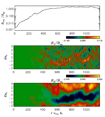
Figure 6.— Time dependence of the root–mean–squared value of the total magnetic field $\mbox{\boldmath$B$}^{\rm tot}$ and spacetime diagrams of $B_{1}(x_{3},t)$ and $B_{2}(x_{3},t)$ [all scaled with respect to $B_{\rm eq}$] from a direct simulation with ${\rm Re}\approx 0.378$, ${\rm Rm}\approx 15.135$ (i.e. ${\rm Pr}\approx 40.0$), $k_{f}/K=3.13$ and ${\rm S_{h}}\approx-1.01$, versus the dimensionless parameter $(t\,v_{\rm rms}\,k_{f})$. The top panel shows the initial exponential growth of the mean magnetic field which saturates subsequently with time. The other two panels demonstrate the episodes of large scale feature in the $x_{3}-$direction, especially in the $B_{2}$ component.

We now report our analysis concerning the growth of mean magnetic field in a background linear shear flow, with non–helical forcing at small scale, for the case when ${\rm Re}<1$ and ${\rm Rm}>1$. This is a particularly interesting regime for the following reasons: (i) it is an important fact to note that in the limit of small ${\rm Re}$ the non–helical forcing has been shown to give rise to non–helical velocity field (see the discussion below Eqn. (46) of Singh & Sridhar (2011)); (ii) For low ${\rm Re}$ the Navier–Stokes Eqn. (2) can be linearized and thus it becomes analytically more tractable problem, as compared to the case of high ${\rm Re}$. Such solutions have been rigorously obtained without the Lorentz forces and have been presented in Singh & Sridhar (2011). So it appears more reasonable to develop a theoretical framework in the limit, ${\rm Re}<1$ and ${\rm Rm}>1$ before one aims to have a theory which is valid for both (${\rm Re}$, ${\rm Rm}$) $>1$. Such thoughts motivated us to perform numerical experiment in this limit to look for the dynamo action. Figures (6–8) display the time dependence of root–mean–squared value of mean magnetic field $B$ and spacetime diagrams of $B_{1}(x_{3},t)$ and $B_{2}(x_{3},t)$ for three different combinations of ${\rm Re}$ and ${\rm Rm}$. These simulations were performed with $128^{3}$ mesh points. We have scaled the magnetic fields in Figs. (6–8) with respect to $B_{\rm eq}$ where $B_{\rm eq}=(\mu_{0}\langle\rho v_{\rm rms}^{2}\rangle)^{1/2}$. Scalings in these Figures have been chosen for compatibility with Figs. (7) and (8) of Brandenburg et al. (2008). Below we list few useful points related to the dynamo action when ${\rm Re}<1$ and ${\rm Rm}>1$ based on careful investigation of Figs. (6–8):

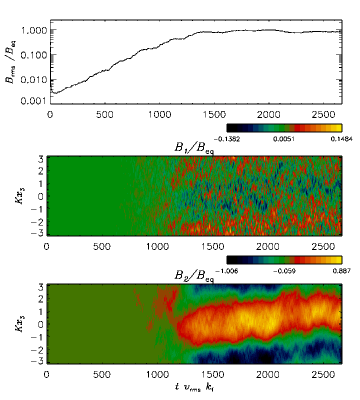
Figure 7.— Same as Fig. (6) but for ${\rm Re}\approx 0.833$, ${\rm Rm}\approx 24.976$ (corresponding to ${\rm Pr}\approx 30.0$), $k_{f}/K=3.13$ and ${\rm S_{h}}\approx-0.23$.

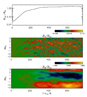
Figure 8.— Same as Fig. (6) but for ${\rm Re}\approx 0.641$, ${\rm Rm}\approx 32.039$ (corresponding to ${\rm Pr}\approx 50.0$), $k_{f}/K=5.09$ and ${\rm S_{h}}\approx-0.60$.

1. Top panels of Figs. (6–8) clearly show the growth of $B_{\rm rms}$ demonstrating the shear dynamo due to non–helical forcing ($B_{\rm rms}^{2}=\left<B^{2}\right>+\left<b^{2}\right>$, where $B$ and $b$ are the magnitudes of the mean and fluctuating magnetic fields respectively). Thus the $B_{\rm rms}-$field may grow either due to $B$ or $b$, or due to both $B$ and $b$.

2. Denoting the magnetic diffusion time scale as $\tau_{\eta}=(\eta k_{f}^{2})^{-1}$ and eddy turn over time scale as $\tau_{\rm edd}=(v_{\rm rms}k_{f})^{-1}$, we write $\tau_{\eta}={\rm Rm}\,\tau_{\rm edd}$. The magnetic fields in these simulations survive for times, say $t=640\,\tau_{edd}$, which for ${\rm Rm}\approx 32$ (corresponding to Fig. (8)) implies, $t\approx 20\,\tau_{\eta}$, i.e., twenty times the diffusion time scale. This is a clear indication of the dynamo action as the magnetic fields survive much longer than the magnetic diffusion time scale.

3. Spacetime diagrams in Figs. (6–8) reveal that the mean magnetic fields start developing only after times which are few times the magnetic diffusion time scale ($\tau_{\eta}$).

4. Although the mean magnetic field starts developing at much later times, $B_{\rm rms}$ starts growing at earlier times. The possibility of the growth of mean–squared field, with no net mean magnetic field at these early times, cannot be ruled out.

Table 2 Summary of the simulations for ${\rm Re}<1$ and ${\rm Rm}>1$

Run	${\rm Re}$	${\rm Rm}$	${-{\rm S_{h}}}$	${\rm Ma}$	Grid	$\eta_{t}/(\eta_{T}{\rm Re}^{2})$	$\eta_{12}/(\eta_{T}{\rm Re}^{2})$	$\eta_{21}/(\eta_{T}{\rm Re}^{2})$
R1	0.393	9.837	0.391	0.10	$128^{3}$	3.657	0.644	0.011
R2	0.396	19.796	0.583	0.10	$144^{3}$	4.735	1.695	0.057
S1	0.592	5.920	0.325	0.15	$144^{3}$	1.508	0.340	0.059
S2	0.598	14.938	0.515	0.15	$144^{3}$	2.110	0.704	0.084
S3	0.598	29.875	0.515	0.15	$144^{3}$	2.400	0.786	0.140
S4	0.603	37.692	0.638	0.15	$144^{3}$	2.435	1.196	0.189

In Table 2 we present results from test–field simulations performed in the regime ${\rm Re}<1$ and ${\rm Rm}>1$. We have runs for two sets of values of fluid Reynolds number, ${\rm Re}$; runs R1, R2 with ${\rm Re}\approx 0.4$ and runs S1–S4 with ${\rm Re}\approx 0.6$. We confirm that all the components of the magnetic diffusivity tensor, $\eta_{t}$, $\eta_{12}$ and $\eta_{21}$, increase with increasing magnetic Reynolds number, ${\rm Rm}$, which is in agreement with Brandenburg et al. (2008). Comparing the numerical values of $\eta$-tensor in Table 2 (with ${\rm Rm}>1$) to those in Table 1 (with ${\rm Rm}<1$), we see that each component of $\eta_{ij}$ increases with ${\rm Rm}$, for range of values considered in this work. For larger values of ${\rm Rm}$ we refer the reader to Brandenburg et al. (2008) where the possibility of the relevant component, $\eta_{21}$, becoming negative at much larger ${\rm Rm}\,(>100)$ was discussed, although the error bars were quite large, and therefore no conclusion could be drawn regarding the mean–field dynamo action. As mentioned earlier, our interest is in the intermediate ${\rm Rm}$ values (5–40), and we show our findings with maximum of ${\rm Rm}$ being below $38$. We note that the component $\eta_{21}$ remains positive even in this parameter regime, thus confirming earlier claims that the shear–current effect cannot be responsible for the observed large–scale dynamo action.

Figure 9.— Panels ($a$–$f$) show magnetic (bold line) and kinetic (dashed line) energy spectra from the direct simulation presented in Fig. (8) with ${\rm Re}\approx 0.641$, ${\rm Rm}\approx 32.039$, $k_{f}/K=5.09$ and ${\rm S_{h}}\approx-0.60$ for different values of $(t\,v_{\rm rms}\,k_{f})$.

It is instructive to know the magnitude of magnetic power at different length scales in the simulations and study its evolution in time. Although the forcing is done at a single length scale, a typical kinetic energy spectrum has a peak at the stirring scale with significantly less power at other length scales (e.g., see dashed lines in various panels of Fig. (9)). We display in Fig. (9) the energy spectra obtained in one of the three simulations (for different combinations of the control parameters, all with ${\rm Re}<1$), corresponding to the one shown in Fig. (8). Thus Figs. (8) and (9) show results obtained from one particular simulation with $128^{3}$ mesh points, ${\rm Re}\approx 0.641$, ${\rm Rm}\approx 32.039$, $k_{f}/K=5.09$ and ${\rm S_{h}}\approx-0.60$. A few noteworthy points are discussed below in detail:

1. Initially the magnetic power is very small as compared to the kinetic power and it is mainly concentrated at large $k$ (i.e. small length scales), as may be seen from panel ($a$) of Fig. (9). Also, there is essentially no magnetic power at small $k$ (i.e. large length scales) at the initial stage of the simulation.

2. The strength of the total magnetic field decreases upto certain time due to dissipation (compare panels ($a$) and ($b$) of Fig. (9)), before it starts building up due to dynamo action.

3. From the top panel of Fig. (8), we see that the root–mean–squared value of the total magnetic field starts growing due to dynamo action ($B_{\rm rms}^{2}=\left<B^{2}\right>+\left<b^{2}\right>$, where $B$ and $b$ are the magnitudes of the mean and fluctuating magnetic fields respectively). As the $B_{\rm rms}-$field may grow either due to $B$ or $b$, or due to both $B$ and $b$, it seems necessary to understand this in more detail. From Fig. (9), it may be seen that the magnetic energy grows at all scales if it starts growing up, till it saturates.

4. The small scale field grows faster, which averages out to zero, and hence does not show up in the spacetime diagrams of Fig. (8). This is generally referred to as the fluctuation dynamo. The growth rate changes and becomes smaller after the fluctuation dynamo saturates (which happens at $t\,v_{\rm rms}\,k_{f}\approx 150$ in Fig. (8) and the corresponding power spectrum at that time is shown in panel ($d$) of Fig. (9)).

5. Although there is non–zero magnetic energy in the large scales when $t\,v_{\rm rms}\,k_{f}\approx 150$ (see panel ($d$) of Fig. (9)), we begin to see some features in the spacetime diagrams of the mean magnetic field (shown in Fig. (8)) only beyond $t\,v_{\rm rms}\,k_{f}\approx 150$. Thus, it is possible that $\mbox{\boldmath$B$}={\bf 0}$ while $\left<B^{2}\right>$ be finite.

6. The mean magnetic field starts developing beyond $t\,v_{\rm rms}\,k_{f}\approx 150$ (which is about five times the magnetic diffusion time scale) and saturates at $t\,v_{\rm rms}\,k_{f}\approx 330$ (see Fig. (8)) after which the magnetic energy essentially stops evolving at all length scales, as may be seen from Fig. (9).

7. When the magnetic energy saturates at some value, we see significant magnetic power at the largest scale.

We recall that in the kinematic stage, the magnetic field at all length scales grow at the same rate, i.e., the magnetic spectrum remains shape invariant (Brandenburg & Subramanian 2005; Subramanian & Brandenburg 2014). From panel ($b$) to panel ($d$) of Fig. (9), the magnetic spectrum evolves in nearly shape invariant manner. During this kinematic stage, much of the magnetic power still lies at small scales, but the power at the largest scales also grows with time. This initial growth of magnetic energy occurs at turbulent (fast) time scale. Towards the end of the kinematic stage, the growth rates of large and small scale magnetic fields become different due to the back reaction from Lorentz forces. The small–scale fields saturate, whereas the large-scale field continues to grow, thus dominating over small–scale fields at much later times; shown in panels ($e$) and ($f$) of Fig. (9).

Figure 10.— Plot of dimensionless initial growth rates, $\gamma^{*}=\gamma/(v_{\rm rms}k_{f})$, of $B_{\rm rms}$ (corresponding to the cases when ${\rm Re}<1$ and ${\rm Rm}>1$) versus $-{\rm S_{h}}$. The ‘$+$’ symbols denote results from direct simulations whereas the bold line shows the slope of the linear trend corresponding to $\gamma^{*}\propto-{\rm S_{h}}$.

It may be seen from the top panels of Figs. (6–8) that $B_{\rm rms}$ shows exponential growth. We denote the initial exponential growth rate of $B_{\rm rms}$ as $\gamma$. It is evident from Fig. (10) that the dimensionless growth rate ($\gamma^{*}=\gamma/(v_{\rm rms}k_{f})$) appears to scale as $\gamma^{*}\propto-{\rm S_{h}}$ in the range of parameters explored in this work. This result is in agreement with (Yousef et al. 2008b; Brandenburg et al. 2008; Heinemann et al. 2011; Richardson & Proctor 2012).

Table 3 Summary of simulations in different parameter regimes

Run	${\rm Re}$	${\rm Rm}$	$k_{f}/K$	${-{\rm S_{h}}}$	${\rm Ma}$	Grid	Comments
A1	0.47	0.47	10.03	1.27	0.0235	$64^{3}$	No dynamo
A2	0.73	0.91	10.03	0.41	0.0727	$128^{3}$	No dynamo
A3	0.76	0.57	1.54	2.78	0.0701	$128^{3}$	No dynamo
B1	41.20	0.82	3.13	0.186	0.258	$64^{3}$	No dynamo
B2	4.65	0.69	10.03	0.0285	0.139	$64^{3}$	No dynamo
B3	4.99	0.75	10.03	0.133	0.150	$64^{3}$	No dynamo
C1	0.59	29.47	5.09	0.12	0.03	$128^{3}$	No dynamo
C2	0.59	29.47	5.09	0.66	0.03	$128^{3}$	Dynamo
C3	0.85	25.50	5.09	0.226	0.129	$128^{3}$	Dynamo
C4	0.75	33.60	10.03	0.236	0.0674	$128^{3}$	Dynamo
D1	1.04	41.66	3.13	0.367	0.13	$128^{3}$	Dynamo
D2	1.79	89.51	5.09	0.215	0.0911	$128^{3}$	Dynamo

In Table 3 we summarize the details of various simulations performed in different parameter regimes. We note that larger shear contributes positively for the mean–field dynamo action; compare the Runs C1 and C2, where shear in C2 is 5 times larger compared to C1, with the rest of the parameters being the same.

4. Conclusions

We performed a variety of numerical simulations exploring different regimes of the control parameters for the shear dynamo problem. The simulations were done for the following three parameter regimes: (i) both (${\rm Re}$, ${\rm Rm}$) $<1$; (ii) ${\rm Re}>1$ and ${\rm Rm}<1$; and (iii) ${\rm Re}<1$ and ${\rm Rm}>1$. These limits, which were never explored in any earlier works, appeared interesting to us for following reasons: first, to compare analytical findings of Singh & Sridhar (2011) with the results of numerical simulations in the parameter regimes when both (${\rm Re}$, ${\rm Rm}$) $<1$; and second, to look for the growth of mean magnetic field in the limit when ${\rm Re}<1$. Exploring the possibility of dynamo action when ${\rm Re}<1$ seems particularly interesting, as, in the limit of small ${\rm Re}$, non–helical forcing has been shown to give rise to non–helical velocity fields (see the discussion below Eqn. (46) of Singh & Sridhar (2011)); whether this is true even in the limit of high ${\rm Re}$ has not been proved yet. Thus performing the simulation in this limit (i.e., ${\rm Re}<1$) with non–helical forcing guarantees the fact that the fluctuating velocity field is also non–helical. Also, for low ${\rm Re}$, the Navier–Stokes Eqn. (2) can be linearized and thus it becomes an analytically more tractable problem, as compared to the case of high ${\rm Re}$. Such solutions have been rigorously obtained without the Lorentz forces, and have been presented in Singh & Sridhar (2011).

In the present paper, we successfully demonstrated that dynamo action is possible in a background linear shear flow due to non–helical forcing when the magnetic Reynolds number is above unity whereas the fluid Reynolds number is below unity, i.e., when ${\rm Re}<1$ and ${\rm Rm}>1$ (see Figs. (6–9)). Few important conclusions may be given as follows:

1. We did not find any dynamo action in the limit when both (${\rm Re}$, ${\rm Rm}$) $<1$ (see Fig. (4)). We note that all the simulations were performed in a fixed cubic domain of size $2\pi^{3}$, and the average outer scales of turbulence in these models were always about ten times smaller than the domain; see Section 3, part A. This scale separation of factor ten might not yet be sufficient, in principle, and the growth at scales larger than the $x_{3}$-extent cannot be ruled out. We computed all the transport coefficients by test–field simulations and compared with the theoretical work of Singh & Sridhar (2011) (see Figs. (1–3)). A good agreement between the theory and the simulations was found for all components of the magnetic diffusivity tensor, $\eta^{\infty}_{ij}$, except for $\eta^{\infty}_{12}$, which is expected to behave in a complicated fashion (Brandenburg et al. 2008; Rüdiger & Kitchatinov 2006; Singh & Sridhar 2011).

2. $\eta^{\infty}_{21}$ was always found to be positive in all the simulations performed in different parameter regimes. This is in agreement with earlier conclusions that the shear–current effect cannot be responsible for dynamo action.

3. There was no evidence of dynamo action in the limit when ${\rm Re}>1$ and ${\rm Rm}<1$ (see Fig. (5)).

4. We demonstrated dynamo action when ${\rm Re}<1$ and ${\rm Rm}>1$ (see Figs. (6–9)). The initial exponential growth rate of $B_{\rm rms}$, $\gamma$, seems to scale linearly with the rate of shear, $|S|$, in the range of parameters explored in this paper (see Fig. (10)); a result which is in agreement with Yousef et al. (2008b); Brandenburg et al. (2008); Heinemann et al. (2011); Richardson & Proctor (2012); Sridhar & Singh (2014).

It’s an intriguing question, what drives the dynamo action in the non-helical turbulence. It has been successfully demonstrated, both, from theoretical and numerical works, that the shear-current effect cannot not be responsible for the observed shear dynamo. In 1976, Kraichnan discussed the possibility of zero–mean $\alpha$ fluctuations, which, together with large scale shear, could possibly give rise to dynamo action in non–helically forced turbulence (Vishniac & Brandenburg 1997; Sokolov 1997; Silant’ev 2000; Proctor 2007). This is known as the incoherent alpha–shear mechanism. Heinemann et al. (2011) have predicted the growth of magnetic energy in a shearing background due to zero–mean $\alpha$ fluctuations, and have obtained scaling relations in agreement to the results from numerical simulations. In a recent analytical study, Sridhar & Singh (2014) have shown that the growth of mean magnetic field is possible due to fluctuating alpha with non–zero correlation times, in a shearing background. They derive the dimensionless parameters controlling the nature of dynamo (or otherwise) action. Numerical computation of these dynamo numbers in simulations of the shear dynamo is being the focus of a future investigation.

References

- Balbus & Hawley (1998) Balbus, S. A., & Hawley, J. F. 1998, Reviews of Modern Physics, 70, 1
- Binney & Tremaine (2008) Binney, J., & Tremaine, S. 2008, Galactic Dynamics: Second Edition (Princeton University Press)
- Blackman (1998) Blackman, E. G. 1998, ApJ, 496, L17
- Brandenburg et al. (2008) Brandenburg, A., Rädler, K.-H., Rheinhardt, M., & Käpylä, P. J. 2008, ApJ, 676, 740
- Brandenburg et al. (2012) Brandenburg, A., Sokoloff, D., & Subramanian, K. 2012, Space Sci. Rev., 169, 123
- Brandenburg & Subramanian (2005) Brandenburg, A., & Subramanian, K. 2005, Phys. Rep., 417, 1
- Heinemann et al. (2011) Heinemann, T., McWilliams, J. C., & Schekochihin, A. A. 2011, Physical Review Letters, 107, 255004
- Hughes & Proctor (2009) Hughes, D. W., & Proctor, M. R. E. 2009, Physical Review Letters, 102, 044501
- Käpylä et al. (2008) Käpylä, P. J., Korpi, M. J., & Brandenburg, A. 2008, A&A, 491, 353
- Kleeorin & Rogachevskii (2008) Kleeorin, N., & Rogachevskii, I. 2008, Phys. Rev. E, 77, 036307
- Krause & Rädler (1980) Krause, F., & Rädler, K.-H. 1980, Mean-field magnetohydrodynamics and dynamo theory
- Leprovost & Kim (2009) Leprovost, N., & Kim, E.-j. 2009, ApJ, 696, L125
- Lithwick (2007) Lithwick, Y. 2007, ApJ, 670, 789
- McWilliams (2012) McWilliams, J. C. 2012, Journal of Fluid Mechanics, 699, 414
- Mitra & Brandenburg (2012) Mitra, D., & Brandenburg, A. 2012, MNRAS, 420, 2170
- Moffatt (1978) Moffatt, H. K. 1978, Magnetic field generation in electrically conducting fluids
- Parker (1979) Parker, E. N. 1979, Cosmical magnetic fields: Their origin and their activity
- Proctor (2007) Proctor, M. R. E. 2007, MNRAS, 382, L39
- Rädler & Stepanov (2006) Rädler, K.-H., & Stepanov, R. 2006, Phys. Rev. E, 73, 056311
- Richardson & Proctor (2012) Richardson, K. J., & Proctor, M. R. E. 2012, MNRAS, 422, L53
- Rogachevskii & Kleeorin (2003) Rogachevskii, I., & Kleeorin, N. 2003, Phys. Rev. E, 68, 036301
- Rogachevskii & Kleeorin (2004) —. 2004, Phys. Rev. E, 70, 046310
- Rogachevskii & Kleeorin (2008) —. 2008, Astronomische Nachrichten, 329, 732
- Rüdiger & Kitchatinov (2006) Rüdiger, G., & Kitchatinov, L. L. 2006, Astronomische Nachrichten, 327, 298
- Shapovalov & Vishniac (2011) Shapovalov, D. S., & Vishniac, E. T. 2011, ApJ, 738, 66
- Silant’ev (2000) Silant’ev, N. A. 2000, A&A, 364, 339
- Singh & Sridhar (2011) Singh, N. K., & Sridhar, S. 2011, Phys. Rev. E, 83, 056309
- Sokolov (1997) Sokolov, D. D. 1997, Astronomy Reports, 41, 68
- Sridhar & Singh (2010) Sridhar, S., & Singh, N. K. 2010, Journal of Fluid Mechanics, 664, 265
- Sridhar & Singh (2014) —. 2014, MNRAS, 445, 3770
- Sridhar & Subramanian (2009a) Sridhar, S., & Subramanian, K. 2009a, Phys. Rev. E, 80, 066315
- Sridhar & Subramanian (2009b) —. 2009b, Phys. Rev. E, 79, 045305
- Subramanian & Brandenburg (2014) Subramanian, K., & Brandenburg, A. 2014, MNRAS, 445, 2930
- Sur & Subramanian (2009) Sur, S., & Subramanian, K. 2009, MNRAS, 392, L6
- Vishniac & Brandenburg (1997) Vishniac, E. T., & Brandenburg, A. 1997, ApJ, 475, 263
- Vishniac & Cho (2001) Vishniac, E. T., & Cho, J. 2001, ApJ, 550, 752
- Wisdom & Tremaine (1988) Wisdom, J., & Tremaine, S. 1988, AJ, 95, 925
- Yousef et al. (2008a) Yousef, T. A., Heinemann, T., Rincon, F., et al. 2008a, Astronomische Nachrichten, 329, 737
- Yousef et al. (2008b) Yousef, T. A., Heinemann, T., Schekochihin, A. A., et al. 2008b, Physical Review Letters, 100, 184501