Direct numerical simulations of rigid body dispersions. I. Mobility/Friction tensors of assemblies of spheres

Abstract

An improved formulation of the ``Smoothed Profile'' method is introduced to perform direct numerical simulations of arbitrary rigid body dispersions in a Newtonian host solvent. Previous implementations of the method were restricted to spherical particles, severely limiting the types of systems that could be studied. The validity of the method is carefully examined by computing the friction/mobility tensors for a wide variety of geometries and comparing them to reference values obtained from accurate solutions to the Stokes-Equation.

I Introduction

The dynamics of particles dispersed in a host solvent, how they react to and affect the fluid motion, is a relevant problem for science as well as engineering fieldsRussel et al. (1992). It is necessary to account for the macroscopic properties of suspensions (such as the viscosity, elastic modulus, and thermal conductivity), as well as the mechanics of protein unfoldingYamakawa (1970), the kinetics of bio-molecular reactionsSon and Lee (2011), and the tumbling motion of bacteriaSokolov and Aranson (2012). As the particles move, they generate long-range disturbances in the fluid, which are transmitted to all other particles. Properly accounting for these hydrodynamic interactions has proven to be a very complicated task due to their non-linear many-body nature.

Several numerical methods have been developed to explicitly include the effect of hydrodynamic interactions in a suspension of particlesBrady and Bossis (1988); Cichocki et al. (1994); Malevanets and Kapral (1999); Hu et al. (2001); Glowinski et al. (2001); Ladd and Verberg (2001); Cates et al. (2004). However, their applicability to non-Newtonian host solvents or solvents with internal degrees of freedom is not straightforward, and in some cases not possible. We have proposed an alternative direct numerical simulation (DNS) method, which we refer to as the Smooth Profile (SP) method, that simultaneously solves for the host fluid and the particles. The coupling between the two motions is achieved through a smooth profile for the particle interfaces. This method is similar in spirit to the fluid particle dynamics methodTanaka and Araki (2000), in which the particles are modeled as a highly viscous fluid. The main benefit of our model is the ability to use a fixed cartesian grid to solve the fluid equations of motion.

The SP method has been successfully used to study the diffusion, sedimentation, and rheology of colloidal dispersions in incompressible fluidsIwashita and Yamamoto (2009a); Kobayashi and Yamamoto (2010); Iwashita and Yamamoto (2009b); Kobayashi and Yamamoto (2011); Hamid and Yamamoto (2013). Recently it has been extended to include self-propelled swimmersMolina et al. (2013) and for compressible host solventTatsumi and Yamamoto (2012). So far, however, only spherical particles were considered. In this paper we extend the SP method to be applicable to arbitrary rigid bodies. We show the validity of the method by computing the mobility/friction tensors for a large variety of geometric shapes. The results are compared to numerical solutions of the Stokes equation, which are essentially exact, as well as experimental data. The agreement with our results is excellent in all cases considered here. Future papers in this series will deal with the dynamical properties of rigid body dispersions in detail, with this work we aim to introduce the basics of the model and show its validity.

II Simulation Model

II.1 Smooth Profile Method for Rigid Bodies

We solve the dynamics of a rigid body in an incompressible Newtonian host fluid using the SP method. The basic idea behind this method is to replace the sharp boundaries between the particles and the fluid with a smooth interface. This allows us to define all field variables over the entire computational domain, and results in an efficient method to accurately resolve the many-body hydrodynamic interactions.

The motion of the host fluid is governed by the incompressible Navier-Stokes equationBatchelor (1967)

$$\left(\partial_{t}+\bm{u}_{f}\cdot\nabla\right)\bm{u}_{f} =\rho_{f}^{-1}\nabla\cdot\bm{\mathsf{\sigma}}_{f}$$ (1)

$$\nabla\cdot\bm{u}_{f} =0$$ (2)

where $\bm{u}_{f}$ is the fluid velocity, $\rho_{f}$ the density, and $\bm{\mathsf{\sigma}}_{f}$ the Newtonian stress tensor

$$\bm{\mathsf{\sigma}}_{f} =-p\bm{\mathsf{I}}+\bm{\mathsf{\sigma}}^{\prime}$$ (3)

$$\bm{\mathsf{\sigma}}_{f}^{\prime} =\eta_{f}\left[\nabla\bm{u}_{f}+\left(\nabla\bm{u}_{f}\right)^{t}\right]$$ (4)

with $p_{f}$ and $\eta_{f}$ the pressure and viscosity of the fluid, respectively.

The motion of the particle is given by the Newton-Euler equationsJosé and Saletan (1998),

$$\dot{\bm{R}}_{I} =\bm{V}_{I} \dot{\bm{\mathsf{Q}}}_{I} =\text{skew}\left(\bm{\Omega}_{I}\right)\cdot\bm{\mathsf{Q}}_{i}$$ (5)

$$M_{I}\dot{\bm{V}}_{I} =\bm{F}_{I} \bm{\mathsf{I}}_{I}\cdot\bm{\Omega}_{I} =\bm{N}_{I}$$ (6)

where $\bm{R}_{I}$, $\bm{V}_{I}$, $\bm{\Omega}_{I}$, and $\bm{\mathsf{Q}}_{I}$, are the center of mass (com) position, velocity, angular velocity, and orientation matrix, respectively, of the $I$-th rigid body ($I=1,\cdots,N$). The total force and torque experienced the particles is denoted as $\bm{F}_{I}$ and $\bm{N}_{I}$, respectively, with $\bm{\mathsf{I}}_{I}$ the moment of inertia tensor and $\text{skew}(\bm{\Omega}_{I})$ the skew-symmetric angular velocity matrix

$$\text{skew}\left(\bm{\Omega}\right)=\begin{pmatrix}0&-\Omega^{z}&\Omega^{y}\\ \Omega^{z}&0&-\Omega^{x}\\ -\Omega^{y}&\Omega^{x}&0\end{pmatrix}$$ (7)

The force (and torque) on each of the particles $\bm{F}_{I}=\bm{F}_{I}^{\text{H}}+\bm{F}_{I}^{\text{C}}+\bm{F}_{I}^{\text{Ext}}$ is comprised of hydrodynamic contributions $\bm{F}^{\text{H}}$, particle-particle interactions (including a core potential to prevent overlap) $\bm{F}^{\text{C}}$, and a possible external field contribution $\bm{F}^{\text{Ext}}$. For the present study, we neglect thermal fluctuations, but they are easily included within the SP formalismIwashita et al. (2008).

The coupling between fluid and particles is obtained by defining a total velocity field $\bm{u}$, with respect to the fluid $\bm{u}_{f}$ and particle $\bm{u}_{p}$ velocity fields, as

$$\bm{u}(\bm{x}) =\left(1-\phi\right)\bm{u}_{f}(\bm{x})+\phi\bm{u}_{p}(\bm{x})$$ (8)

$$\phi\bm{u}_{p}(\bm{x}) =\sum_{I}\phi_{I}(\bm{x};\bm{R}_{I},\bm{\mathsf{Q}}_{I})\left[\bm{V}_{I}+\bm{\Omega}_{I}\times\bm{r}_{I}\right]$$ (9)

where $\phi_{I}(\bm{x};\bm{R}_{I},\bm{\mathsf{Q}}_{I})$ is a suitably defined SP function ($0\leq\phi_{I}\leq 1$) that interpolates between fluid and particle domains (as described below), and $\bm{r}_{I}=\bm{x}-\bm{R}_{I}$. The modified Navier-Stokes equation which governs the evolution the total fluid velocity field (host fluid $+$ particle) is given byNakayama and Yamamoto (2005)

$$\left(\partial_{t}+\bm{u}\cdot\nabla\right)\bm{u} =\rho^{-1}\nabla\cdot\bm{\mathsf{\sigma}}+\phi\bm{f}_{p}$$ (10)

$$\nabla\cdot\bm{u}_{f} =0$$ (11)

with $\rho=\rho_{f}$ and $\eta=\eta_{f}$. The stress tensor is defined as in eq. (3), but in terms of the total fluid velocity $\bm{u}$.

The scheme used to solve the equations of motion is the same fractional-step algorithm introduced in refNakayama et al. (2008)., with minor modifications needed to account for the non-spherical geometry of the particles. Let $\bm{u}^{n}$ be the velocity field at time $t_{n}=nh$ ($h$ the time interval). We first solve for the advection and hydrodynamic viscous stress terms, and propagate the particle positions (orientations) using the current particle velocities

$$\bm{u}^{*} =\bm{u}^{n}+\int_{t_{n}}^{t_{n}+h}\text{d}s\,\nabla\cdot\left[\rho^{-1}\bm{\mathsf{\sigma}}-\bm{u}\bm{u}\right]$$ (12)

$$\bm{R}_{I}^{n+1} =\bm{R}_{I}^{n}+\int_{t_{n}}^{t_{n}+h}\text{d}s\,\bm{V}_{I}$$ (13)

$$\bm{\mathsf{Q}}_{I}^{n+1} =\bm{\mathsf{Q}}_{I}^{n}+\int_{t_{n}}^{t_{n}+h}\text{d}s\,\text{skew}\left(\bm{\Omega}_{I}\right)\cdot\bm{\mathsf{Q}}_{I}$$ (14)

Given the dependence of the profile function on the particle position and orientation, we must also update the particle velocity field to

$$\phi\bm{u}_{p}^{*}(\bm{x})=\sum_{I}\phi^{n+1}_{I}(\bm{x})\left[\bm{V}_{I}^{n+1}+\bm{\Omega}_{I}\times\bm{r}_{I}^{n+1}\right]$$ (15)

Next, we compute the hydrodynamic force and torque exerted by the fluid on the particles, by assuming momentum conservation. The time integrated hydrodynamic force and torque over a period $h$ are equal to the momentum exchange over the particle domain

$$\left[\int_{t_{n}}^{t_{n}+h}\text{d}s\,\bm{F}_{I}^{\text{H}}\right] =\int\text{d}\bm{x}\,\rho\phi_{I}^{n+1}\left(\bm{u}^{*}-\bm{u}_{p}^{*}\right)$$ (16)

$$\left[\int_{t_{n}}^{t_{n}+h}\text{d}s\,\bm{N}_{I}^{\text{H}}\right] =\int\text{d}\bm{x}\,\left[\bm{r}_{I}^{n+1}\times\rho\phi_{I}^{n+1}\left(\bm{u}^{*}-\bm{u}_{p}^{*}\right)\right]$$ (17)

From this, and any other forces on the rigid bodies, we update the velocities of the particles as

$$\bm{V}_{I}^{n+1} =\bm{V}_{I}^{n}+M_{I}^{-1}\int_{t_{n}}^{t_{n}+h}\text{d}s\,\left[\bm{F}_{I}^{\text{H}}+\bm{F}_{I}^{\text{C}}+\bm{F}_{I}^{\text{Ext}}\right]$$ (18)

$$\bm{\Omega}_{I}^{n+1} =\bm{\Omega}_{I}^{n}+\bm{\mathsf{I}}_{I}^{-1}\int_{t_{n}}^{t_{n}+h}\cdot\left[\bm{N}_{I}^{\text{H}}+\bm{N}_{I}^{\text{C}}+\bm{N}_{I}^{\text{Ext}}\right]$$ (19)

Finally, the particle rigidity is imposed on the total fluid velocity through the body force in the Navier-Stokes equation

$$\bm{u}^{n+1} =\bm{u}^{*}+\left[\int_{t_{n}}^{t_{n}+h}\text{d}s\,\phi\bm{f}_{p}\right]$$ (20)

$$\left[\int_{t_{n}}^{t_{n}+h}\text{d}s\,\phi\bm{f}_{p}\right] =\phi^{n+1}\left(\bm{u}_{p}^{n+1}-\bm{u}^{*}\right)-\frac{h}{\rho}\nabla p_{p}$$ (21)

with the pressure due to the rigidity constraint obtained from the incompressibility condition $\nabla\cdot\bm{u}^{n+1}=0$.

II.2 Rigid Body Representation

For computational simplicity, we consider each particle ($I$) as being composed of a rigid collection of $n_{I}$ spherical beads (see fig.1), with position, velocities, and angular velocities given by $\bm{R}_{i}$, $\bm{V}_{i}$, and $\bm{\Omega}_{i}$. We use upper and lowercase variables to differentiate between rigid body particles and the spherical beads used to construct them, as well as the shorthand $i\in I$ to refer to the $n_{I}$ beads belonging to the rigid body $I$. The rigidity constraint on the bead velocities is given by

$$\bm{V}_{i} =\bm{V}_{I}+\bm{\Omega}_{I}\times\bm{G}_{i}$$ (22)

$$\bm{\Omega_{i}} =\bm{\Omega}_{I}$$ (23)

where $\bm{G}_{i}=\bm{R}_{i}-\bm{R}_{I}$ is the distance vector from the com of the rigid body ($\bm{R}_{I}$) to the bead's com ($\bm{R}_{i}$). The rigidity constraint on the position of the beads requires that the relative distances between any two of them remain constant. Thus, the $\bm{G}_{i}$ vectors, expressed within the reference frame of the particle $\widetilde{\bm{G}}_{i}$, are constants of motion

$$\widetilde{\bm{G}}_{i}=\bm{\mathsf{Q}}_{I}^{\text{t}}\cdot\bm{G}_{i}=\text{constant}$$ (24)

where $\bm{\mathsf{A}}^{t}$ is the matrix transpose of $\bm{\mathsf{A}}$. The individual positions of the beads can be directly obtained from the position and orientation of the rigid body to which they belongs through

$$\bm{R}_{i} =\bm{R}_{I}+\bm{G}_{i}$$ (25)

$$\bm{G}_{i} =\bm{\mathsf{Q}}_{I}\cdot\widetilde{\bm{G}}_{i}$$ (26)

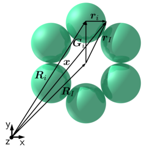
Figure 1: Rigid body representation as arbitrary collection of spherical beads.

The beads should only be considered as a computational bookkeeping device, used to map the rigid particles onto the computational grid used to solve the fluid equations of motion. We are free to chose any representation of the rigid body.

The advantage of this spherical-bead representation is the ease with which the smooth profile function $\phi_{I}$ of an arbitrary rigid body can be defined. We start with the profile function for spherical particles introduced in ref. Nakayama and Yamamoto (2005)

$$\phi_{i}\left(\bm{x}\right) =\frac{h\left[\left(a+\xi/2\right)-r_{i}\right]}{h\left[\left(a+\xi/2\right)-r_{i}\right]+h\left[r_{i}-\left(a-\xi/2\right)\right]}$$ (27)

$$h(x) =\begin{cases}\exp{\left(-\Delta^{2}/x^{2}\right)}&x\geq 0\\ 0&x<0\end{cases}$$ (28)

where $\bm{r}_{i}=\bm{x}-\bm{R}_{i}$ is the distance vector from the sphere center to the field point of interest, $a$ is the radius of the spheres, and $\xi$ is the thickness of the fluid-particle interface. We then define the smooth profile function of the rigid body as

$$\phi_{I}(\bm{x}) =\sum_{i\in I}\frac{\phi_{i}(\bm{x})}{\text{max}\left(\sum_{j\in I}\phi_{j}\left(\bm{x}\right),1\right)}$$ (29)

The normalization factor in eq. (29) is required to avoid double-counting in the case of overlap between beads belonging to the same rigid particle (beads belonging to different particles are prevented from overlapping by the core potential in $\bm{F}^{C}$). We note that this representation of particles as rigid assemblies of spheres does not impose any constraints on the particle geometries, because the constituent beads are free to overlap with each other.

III Stokes Drag

If the dispersion under consideration is such that the inertial forces are negligible compared to the viscous forces, i.e. when the particle Reynolds number is vanishingly small $\text{Re}=\rho UL/\eta\ll 1$ ($U$ and $L$ being the characteristic velocity and length scales), the incompressible Navier-Stokes equation (eq. (1)) reduces to the Stokes equationBatchelor (1967)

$$\eta\nabla^{2}\bm{u} =\nabla p+\bm{f}^{\text{Ext}}$$ (30)

with $\bm{f}^{\text{ext}}$ any external forces on the fluid. Due to the linear nature of this equation, the force (torque) exerted by the fluid on the particles is also linear in the their velocitiesKim and Karrila (2005); Dhont (1996)

$$\bm{\mathsf{F}} =\bm{\mathsf{Z}}\cdot\bm{\mathsf{U}}$$ (31)

$$\bm{\mathsf{U}} =\bm{\mathsf{M}}\cdot\bm{\mathsf{F}}$$ (32)

where $\bm{\mathsf{F}}=\left(\bm{F}_{1},\ldots,\bm{F}_{N},\bm{N}_{1},\ldots,\bm{N}_{N}\right)$ and $\bm{\mathsf{U}}~{}=~{}\left(\bm{V}_{1},\ldots,\bm{V}_{N},\bm{\Omega}_{1},\ldots,\bm{\Omega}_{N}\right)$ are $6N$ dimensional force and velocity vectors, and $\bm{\mathsf{Z}}$ and $\bm{\mathsf{M}}=\bm{\mathsf{Z}}^{-1}$ are the friction and mobility matrices, respectively

$$\bm{\mathsf{Z}} =\begin{pmatrix}\bm{\mathsf{Z}}^{tt}&\bm{\mathsf{Z}}^{tr}\\ \bm{\mathsf{Z}}^{rt}&\bm{\mathsf{Z}}^{rr}\end{pmatrix}$$ (33)

$$=\begin{pmatrix}\bm{\mathsf{\zeta}}^{tt}_{11}&\cdots&\bm{\mathsf{\zeta}}^{tt}_{1N}&\bm{\mathsf{\zeta}}^{tr}_{11}&\cdots&\bm{\mathsf{\zeta}}^{tr}_{1N}\\ \vdots&\ddots&\vdots&\vdots&\ddots&\vdots\\ \bm{\mathsf{\zeta}}^{tt}_{N1}&\cdots&\bm{\mathsf{\zeta}}^{tt}_{NN}&\bm{\mathsf{\zeta}}^{tr}_{N1}&\cdots&\bm{\mathsf{\zeta}}^{tr}_{NN}\\[6.00006pt] \bm{\mathsf{\zeta}}^{rt}_{11}&\cdots&\bm{\mathsf{\zeta}}^{rt}_{1N}&\bm{\mathsf{\zeta}}^{rr}_{11}&\cdots&\bm{\mathsf{\zeta}}^{rr}_{1N}\\ \vdots&\ddots&\vdots&\vdots&\ddots&\vdots\\ \bm{\mathsf{\zeta}}^{rt}_{N1}&\cdots&\bm{\mathsf{\zeta}}^{rt}_{NN}&\bm{\mathsf{\zeta}}^{rr}_{1N}&\cdots&\bm{\mathsf{\zeta}}^{rr}_{NN}\end{pmatrix}$$ (34)

$$\bm{\mathsf{M}} =\begin{pmatrix}\bm{\mathsf{M}}^{tt}&\bm{\mathsf{M}}^{tr}\\ \bm{\mathsf{M}}^{rt}&\bm{\mathsf{M}}^{rr}\end{pmatrix}$$ (35)

$$=\begin{pmatrix}\bm{\mathsf{\mu}}^{tt}_{11}&\cdots&\bm{\mathsf{\mu}}^{tt}_{1N}&\bm{\mathsf{\mu}}^{tr}_{11}&\cdots&\bm{\mathsf{\mu}}^{tr}_{1N}\\ \vdots&\ddots&\vdots&\vdots&\ddots&\vdots\\ \bm{\mathsf{\mu}}^{tt}_{N1}&\cdots&\bm{\mathsf{\mu}}^{tt}_{NN}&\bm{\mathsf{\mu}}^{tr}_{N1}&\cdots&\bm{\mathsf{\mu}}^{tr}_{NN}\\[6.00006pt] \bm{\mathsf{\mu}}^{rt}_{11}&\cdots&\bm{\mathsf{\mu}}^{rt}_{1N}&\bm{\mathsf{\mu}}^{rr}_{11}&\cdots&\bm{\mathsf{\mu}}^{rr}_{1N}\\ \vdots&\ddots&\vdots&\vdots&\ddots&\vdots\\ \bm{\mathsf{\mu}}^{rt}_{N1}&\cdots&\bm{\mathsf{\mu}}^{rt}_{NN}&\bm{\mathsf{\mu}}^{rr}_{1N}&\cdots&\bm{\mathsf{\mu}}^{rr}_{NN}\end{pmatrix}$$ (36)

where the off-diagonal matrices are related through the Lorentz reciprocal relations byKim and Karrila (2005)

$$\bm{\mathsf{Z}}^{rt} =\left(\bm{\mathsf{Z}}^{tr}\right)^{\text{t}}$$ (37)

$$\bm{\mathsf{M}}^{rt} =\left(\bm{\mathsf{M}}^{tr}\right)^{\text{t}}$$ (38)

The symmetric block matrices $\bm{\mathsf{Z}}$ ($\bm{\mathsf{M}}$) are composed of $3\times 3$ friction (mobility) matrices $\bm{\mathsf{\zeta}}^{tt}_{ij}$, $\bm{\mathsf{\zeta}}^{tr}_{ij}$, $\bm{\mathsf{\zeta}}^{rt}_{ij}$, and $\bm{\mathsf{\zeta}}^{rr}_{ij}$ which couple the translational and rotational motion of particle $i$ with that of particle $j$. Thus, the whole problem of solving the dynamical equations of motion for a suspension of spheres in the Stokes regime reduces to calculating the mobility or friction matrix. For a single spherical particle, translating (rotating) in an unbounded fluid under stick-boundary conditions, the translational $\zeta^{t}$ and rotational $\zeta^{r}$ friction coefficients are obtained from an exact solution of the Stokes equation asDhont (1996)

$$\zeta^{t} =\frac{1}{\mu^{t}}=6\pi\eta a$$ (39)

$$\zeta^{r} =\frac{1}{\mu^{r}}=8\pi\eta a^{3}$$ (40)

Exact solutions to the friction or resistance problem of two or three spherical particles are knownJeffrey and Onishi (1984); Kim and Mifflin (1985); Kim (1987), but for arbitrary many-particle systems, the complex non-linear nature of the hydrodynamic interactions makes it impossible to find a general solution. However, several methods have been developed to obtain accurate estimates for the mobility and friction matrices. Two of the most popular approaches are the method of reflections and the method of induced forcesDhont (1996); Cichocki et al. (1994). The former relies on a power series expansion of the flow field, in terms of the inverse particle distances ($a/r_{ij}$), while the latter uses a multipole expansion of the force densities induced at the particle surface, with the truncation scheme determined by the angular dependence of the flow field ($l=1,\ldots,L$). As an example, the popular Rotne-Prager (RPY) approximation to the mobility tensor can be obtained using the method of reflections, by truncating the hydrodynamic interactions to third order, which corresponds to a pair-wise representation

$$\bm{\mathsf{\mu}}_{ij}^{tt} =\begin{cases}\mu^{t}\bm{\mathsf{I}}&i=j\\ \mu^{t}\left[\frac{3}{4}\left(\bm{\mathsf{I}}+\hat{\bm{r}}_{ij}\hat{\bm{r}}_{ij}\right)+\frac{1}{2}\left(\frac{a}{r_{ij}}\right)^{3}\left(\bm{\mathsf{I}}-3\hat{\bm{r}}_{ij}\hat{\bm{r}}_{ij}\right)\right]&i\neq j\end{cases}$$ (41)

We will compare our DNS results with those obtained using the method of induced forces, using the freely available HYDROLIB libraryHinsen (1995). Calculations of the friction coefficients for a sedimenting array of spherical clusters, using the induced force method truncated to third order ($L=3$), gives an error of less than $1\%$ with respect to the experimental resultsCichocki and Hinsen (1995). We therefore consider these values as the exact solution to the Stokes equation (SE). Finally, we note that neither the method of reflections nor the induced force method is able to directly take into account lubrication forces, caused by the relative motion of particles at short distances, as they require the high-order terms to be included in both expansions. Following Durlofsky et al.Durlofsky et al. (1987), these contributions are usually added to the friction matrix by assuming a pairwise superposition approximation. In this work we will consider only the collective motion of a rigid agglomerate of spheres, so that lubrication effects need not be considered.

IV Results

In what follows we report the friction coefficients for a variety of non-spherical particles under steady translation (rotation) through a fluid. The numerical simulations are performed in three dimensions under periodic boundary conditions. The modified Navier-Stokes equation (eq.(10)) is discretized with a dealiased Fourier spectral scheme in space and an Euler scheme in time. The motion of the particles is integrated using a second order Adams-Bashforth scheme. The lattice spacing $\Delta$ is taken as unit of length, the unit of time is given by $\rho\Delta^{2}/\eta$, with $\rho=1$ and $\eta=1$ the density and viscosity of the fluid. The integration time step is $h=7.5\times 10^{-2}$. We only consider neutrally bouyant particles, $\rho_{p}=\rho$, so gravity effects are not considered Furthermore, we are only interested in single particle motion, so the particle-particle interactions and external field contributions can be ignored $\bm{F}^{\text{Ext}}=\bm{F}^{\text{C}}=0$.

The rigid particles are constructed as rigid agglomerates of non-overlapping spherical beads of equal radius $a$. We use a bead radius of $a=2,4$ and a system size of $L=128,256$ (depending on the particle geometry); the interfacial thickness is $\zeta=2$ in all cases. The particle velocity $\mathsf{U}^{\alpha}$ is fixed throughout the simulation and the steady-state forces $\mathsf{F}^{\beta}$, which are purely hydrodynamic in nature, are measured in order to obtain the friction coefficients $\zeta^{\alpha\beta}$. All results are given in terms of the kinetic form factors $\mathsf{K}^{\alpha\beta}$, defined as

$$\bm{\mathsf{Z}}=\begin{pmatrix}\bm{\mathsf{K}}^{tt}\zeta^{t}\phantom{/\zeta^{t}}&\bm{\mathsf{K}}^{tr}\zeta^{r}/\zeta^{t}\\ \bm{\mathsf{K}}^{rt}\zeta^{r}/\zeta^{t}&\bm{\mathsf{K}}^{rr}\zeta^{r}\phantom{/\zeta^{t}}\end{pmatrix}$$ (42)

such that $\bm{\mathsf{K}}^{tt}$ ($\bm{\mathsf{K}}^{rr}$) expresses the force (torque) on the agglomerates relative the force (torque) experienced by a spherical particle of equal volume (radius $a_{e}$) moving (rotating) at the same velocity (angular velocity) and under the same boundary conditions. We use the general term, friction tensor or matrix, to refer to both $\bm{\mathsf{Z}}$ and $\bm{\mathsf{K}}$.

IV.1 Spherical Agglomerates

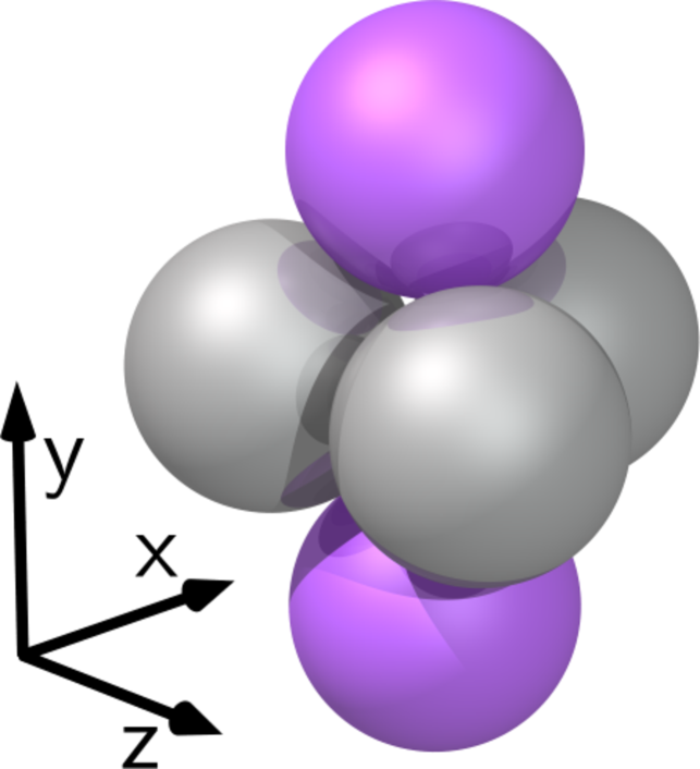
(a) hcp₅

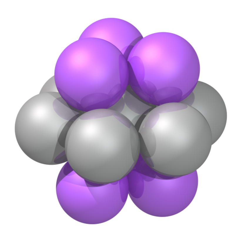
(b) hcp₁₃

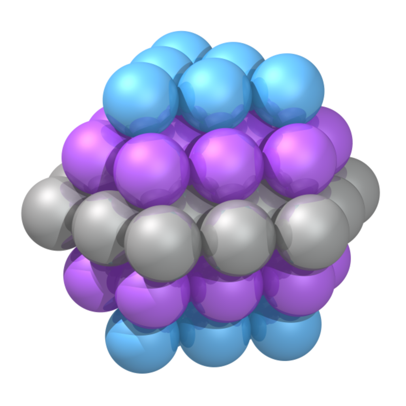
(c) fcp₅₅

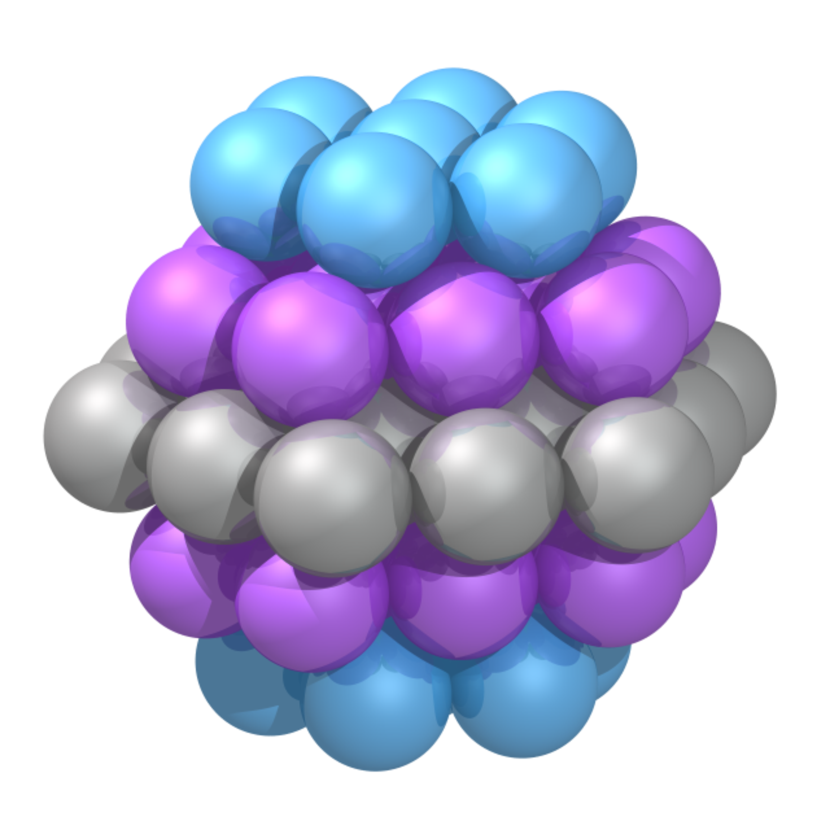
(d) hcp₅₇

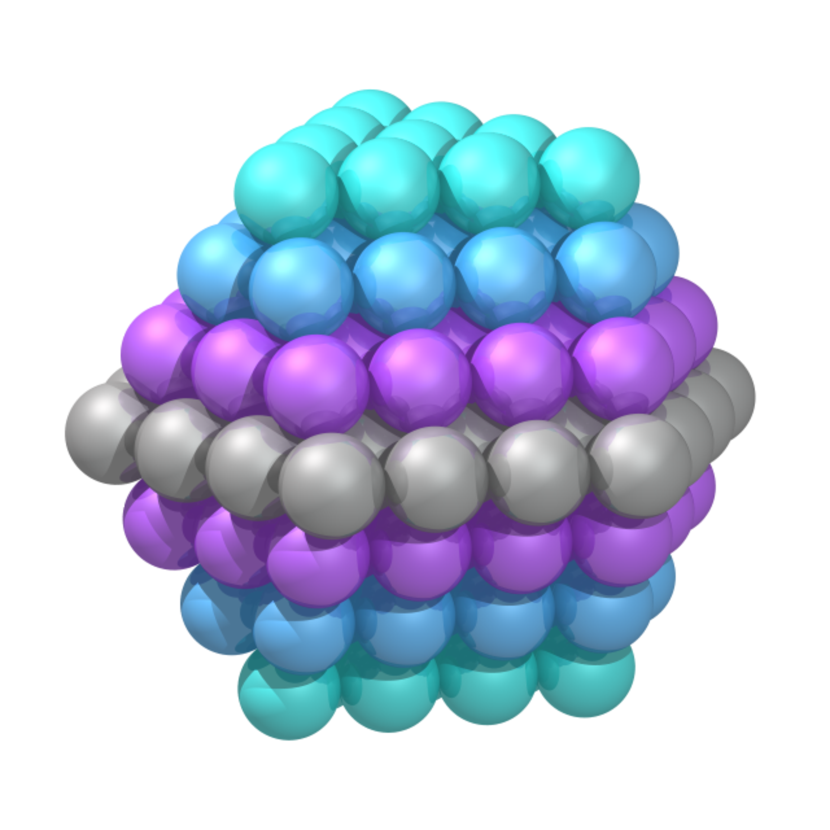
(e) hcp₁₄₇

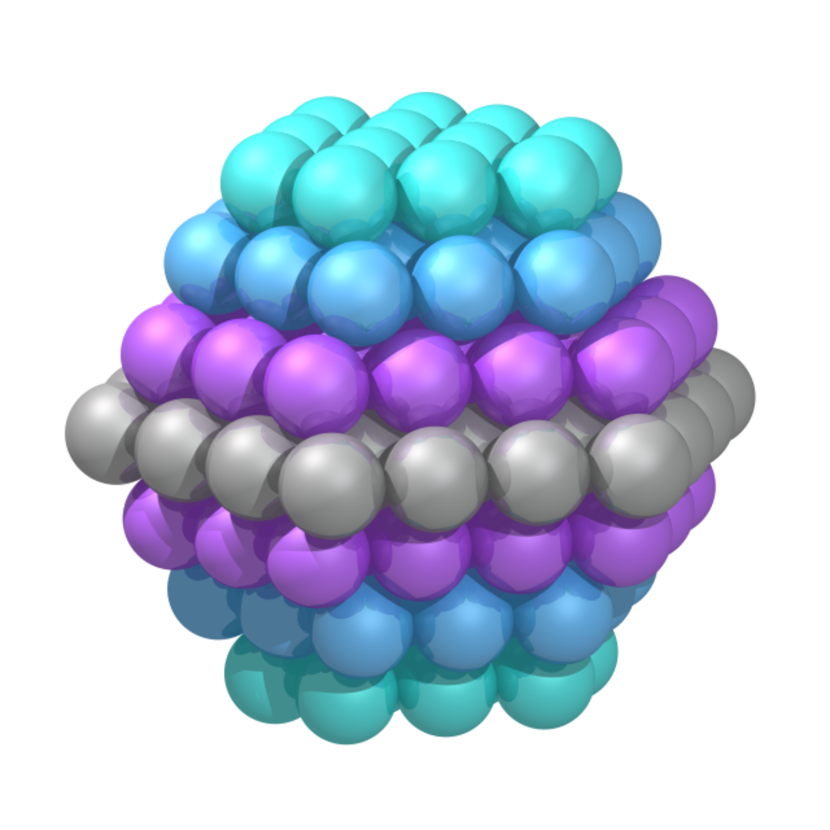
(f) hcp₁₅₃

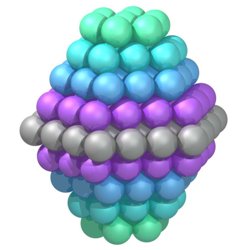
(g) hcp₁₆₇

Figure 2: (color online) Closed-packed (hcp and fcc) arrays of spherical particles. Colors are assigned to the individual layers as a visual guide.

We begin by measuring the friction coefficients of the spherical agglomerates studied experimentally in ref Cichocki and Hinsen (1995). The agglomerates where constructed to obtain semi-spherical geometries by gluing together from two to $167$ spherical beads of equal radius within a closest-packing arrangement (using either hcp or fcc lattices). The spherical agglomerates for $N\geq 5$ are shown in Fig. 2. The system parameters are $a=2$, $L=128$, and $V^{\alpha}=0.02$ ($\alpha=y,z$), which gives a Reynolds number of $\leq 0.44$. Given the symmetry of the particles, the friction matrix is diagonal, with only two distinct coefficients

$$\bm{\mathsf{K}}^{tt}=\begin{pmatrix}\mathsf{K}^{zz}&0&0\\ 0&\mathsf{K}^{yy}&0\\ 0&0&\mathsf{K}^{zz}\end{pmatrix}$$ (43)

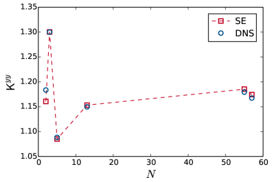
Figure 3: (color online) Friction coefficients $\mathsf{K}^{yy}$ for several closed-packed arrays of spherical particles as a function of size (number of spheres). Results obtained from DNS calculations (circle) are compared to the exact solution to the Stokes equation (square).

$N$	$a/a_{e}$	$\mathsf{K}_{SE}^{yy}$	$\mathsf{K}_{DNS}^{yy}$	$\mathsf{K}_{SE}^{zz}$	$\mathsf{K}_{DNS}^{zz}$
2	$1.26$	$1.161$	$1.184$	$1.025$	$1.051$
3	$1.44$	$1.300$	$1.300$	$1.074$	$1.081$
5	$1.71$	$1.085$	$1.088$	$1.172$	$1.173$
13	$2.35$	$1.153$	$1.150$	$1.153$	$1.148$
55	$3.80$	$1.185$	$1.179$	$1.185$	$1.175$
57	$3.84$	$1.174$	$1.167$	$1.178$	$1.167$
147	$5.28$	—	$1.198$	—	$1.195$
153	$5.35$	—	$1.184$	—	$1.186$
167	$5.50$	—	$1.156$	—	$1.227$

Table 1: Friction coefficients for motion parallel and perpendicular to the vertical $y$-axis for all the closed-packed arrays, as given by our DNS method and the exact solution to the SE.

Precise experimental measurements are available for these systems, but they should not be compared directly to our simulation results due to the mismatch in boundary conditions, particularly for the larger agglomerates. The friction coefficients for movement along the vertical $y$-axis are given in fig 3, where they are compared to the exact (SE) results. The complete set of values for the two independent friction coefficients are given in table 1. For the larger systems, $N\geq 147$, the HYDROLIB library does not converge if periodic boundary conditions are used, so no reference data is given. Our results show excellent agreement with the available SE values, differentiating between nearly identical agglomerates which differ in volume by only a few percent. In all cases, the difference between our results and the reference values are less than $2\%$, which is the comparable with the error estimates of the actual experiments.

IV.2 Non-Spherical Agglomerates

We now consider the friction coefficients for a series of non-spherical regular-shaped agglomerates. The simulation protocol is exactly the same as for the spherical agglomerates considered above. In total, we study six different families of configurations, shown schematically in fig. 4, v-shaped, w-shaped, h-shaped, hexagonal and rectangular arrays. The v- and w-shaped configurations vary in the number of particles ($N=3,4,5$), as well as the branching angle $\theta$. For the h-shaped and hexagonal configurations only the branching angle is varied, the number of particles is fixed to six. For the rectangular $(l\times m)\times n$ arrays, the maximum number of particles in any dimension is four. In total, we have considered $84$ different geometric configurations. Details on the construction of the agglomerates, as well as experimental data for the kinematic form factors, can be found in ref. Niida and Ohtsuka (1997).

(a) v-shaped (even)

(b) v-shaped (odd)

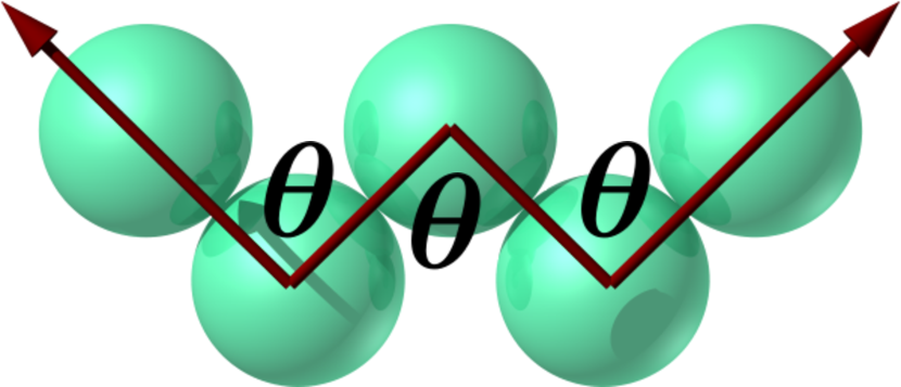
(c) w-shaped

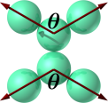
(d) h-shaped

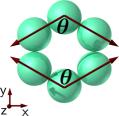
(e) hexagonal

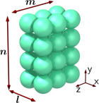
(f) rectangular

Figure 4: (color online) Non-spherical agglomerates for various regular shaped geometries.

The total friction matrix $\bm{\mathsf{K}}$ is block diagonal for all the geometrical configurations considered here, except for the case of v- and w-shaped particles, for which a slight coupling between translation and rotation can be observed: $(\mathsf{K}^{rt})^{xz}$ and $(\mathsf{K}^{rt})^{zx}\neq 0$. For the moment, however, we consider only translational motion. Due to the symmetry of the particles, the friction matrix $\bm{\mathsf{K}}^{tt}$ is again diagonal

$$\bm{\mathsf{K}}^{tt} =\mathsf{K}^{\alpha\beta}\bm{\mathsf{\delta}}_{\alpha\beta}$$ (44)

We have computed the friction coefficients for motion parallel to the vertical $y$ axis for all the systems, the full friction matrix is only measured for the h-shaped and hexagonal agglomerates. Our results are summarized in fig. 5, along with the experimental data, and the exact solutions for both a periodic and an infinite system. Although our DNS results should only be compared with the SE solutions under equivalent boundary conditions, the periodicity effects for the systems considered here are small, being of the same order of magnitude as the errors in the experiments. The relative error of the DNS results (compared to experiments) is less than $5\%$ for all configurations. A comparison of our results with the exact SE values under periodic boundary conditions show almost perfect agreement, considerably better than that of experiments with the exact SE values for an infinite system.

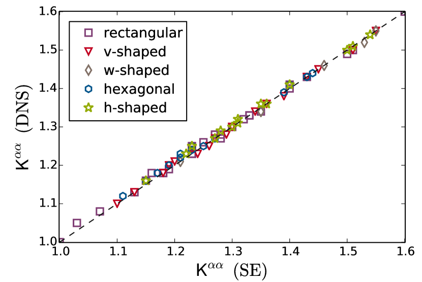
(a) DNS versus SE

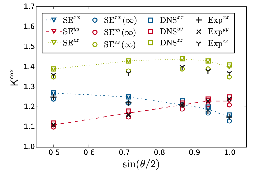
(b) hexagonal

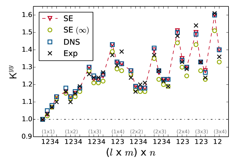
(c) rectangular

Figure 5: (color online) Friction coefficients for various non-spherical regular-shaped agglomerates. (a) All the friction coefficients computed with the DNS method as a function of the exact SE values. (b) The friction coefficients for the hexagonal shaped agglomerates as a function of their vertical dimension. (c) Vertical friction coefficients for rectangular $(l\times m)\times n$ arrays as a function of height $n$. Values obtained from the exact solution to the SE, for both periodic and unbounded $(\infty)$ systems, as well as experimental values, are also shown in (b) and (c).

The friction coefficients $\mathsf{K}^{\alpha\alpha}_{\text{DNS}}$ of all the configurations are plotted in fig. 5(a) with respect to the exact SE value for a system with the same periodic boundary conditions $\mathsf{K}^{\alpha\alpha}_{\text{SE}}$. The results clearly show the accuracy of our method, as $\mathsf{K}^{\alpha\alpha}_{\text{DNS}}=\mathsf{K}^{\alpha\alpha}_{\text{SE}}$ within $\lesssim 2\%$. Detailed results for the hexagonal particles are given in fig. 5(b), where the three form factors $\mathsf{K}^{\alpha\alpha}$ are plotted as a function of the vertical dimensions of the agglomerate ($\sin{\theta/2}$). The DNS results show almost perfect agreement with the exact SE results. The difference among the frictions coefficients and their dependence on the branching angle is very accurately reproduced. Finally, the form factors for the rectangular $(l\times m)\times n$ arrays are plotted in fig. 5(c), as a function of increasing vertical height $n$. As expected, the agreement with the exact results is very good, and we are able to accurately distinguish between particles with the same cross-sectional area $(l\times n)$.

IV.3 Chiral Structures

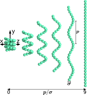
Figure 6: (color online) Helical structures of varying pitch $p\sigma$ ($\sigma$ is the particle diameter), with constant length ($30$ beads) and number of turns ($3$).

Up to now, we have considered symmetric particles for which the translational and rotational motion are only weakly coupled, if at all. Here we will analyze chiral structures which exhibit a very strong coupling between the two motions. We consider left-handed helices composed of a fixed number of beads ($30$) and turns ($3$), which vary only in their degree of pitch $p$ (surface to surface distance between turns). The pitch will then vary in the range $0\leq p\leq 9$, with $p=0$ corresponding to a packed configuration (hollow cylinder), and $p=9$ to a linear chain (see fig. 6). The simulation protocol is slightly modified with respect to the previous systems, we now consider beads of radius $a=4$ and a simulation box size of $L=256$. To compute the complete friction matrix, we now require six different simulations for each helical geometry: three at fixed velocity $V^{\alpha}=-10^{-3}$ and three at fixed angular velocity $\Omega^{\alpha}=10^{-4}$ ($\alpha=x,y,z$).

The friction matrices obtained from the DNS simulations, together with the exact SE values, for a helix with pitch $p/\sigma=6.5$ ($\sigma=2a$ the diameter of the beads) are given in eqs. (45)–(47)

$$\bm{\mathsf{K}}^{tt}_{\text{DNS}} =\left(\begin{smallmatrix}-3.44&-1.38\times 10^{-2}&-7.53\times 10^{-3}\\ -1.35\times 10^{-2}&-2.28&-4.21\times 10^{-2}\\ -7.44\times 10^{-3}&-4.21\times 10^{-2}&-3.47\end{smallmatrix}\right)$$ (45)

$$\bm{\mathsf{K}}^{tt}_{\text{SE}\phantom{S}} =\left(\begin{smallmatrix}-3.4&-1.3\times 10^{-2}&-7.55\times 10^{-3}\\ -1.3\times 10^{-2}&-2.22&-4.01\times 10^{-2}\\ -7.55\times 10^{-3}&-4.01\times 10^{-2}&-3.42\end{smallmatrix}\right)$$

$$\bm{\mathsf{K}}^{rr}_{\text{DNS}} =\left(\begin{smallmatrix}-5.67\times 10^{1}&-6.42\times 10^{-1}&2.04\times 10^{-1}\\ -5.59\times 10^{-1}&-2.61&-1.62\\ 1.56\times 10^{-1}&-1.58&-5.6\times 10^{1}\end{smallmatrix}\right)$$ (46)

$$\bm{\mathsf{K}}^{rr}_{\text{SE}\phantom{S}} =\left(\begin{smallmatrix}-5.64\times 10^{1}&-5.3\times 10^{-1}&1.55\times 10^{-1}\\ -5.3\times 10^{-1}&-2.78&-1.63\\ 1.55\times 10^{-1}&-1.63&-5.6\times 10^{1}\end{smallmatrix}\right)$$

$$\bm{\mathsf{K}}^{rt}_{\text{DNS}} =\left(\begin{smallmatrix}3.94&6.27\times 10^{-1}&-1.19\\ -3.1&-5.39&-9.4\\ -6.03\times 10^{-1}&1.94&1.34\end{smallmatrix}\right)$$ (47)

$$\bm{\mathsf{K}}^{rt}_{\text{SE}\phantom{S}} =\left(\begin{smallmatrix}3.92&6.63\times 10^{-1}&-9.26\times 10^{-1}\\ -2.99&-5.21&-9.22\\ -9.27\times 10^{-1}&2.04&1.33\end{smallmatrix}\right)$$

The complex nature of the fluid flow generated by the motion of the body is clearly evident in the form of the friction matrices. The translational (rotational) friction matrix $\bm{\mathsf{K}}^{tt}$ ($\bm{\mathsf{K}}^{rr}$) is no longer diagonal, eqs. (45) and (46), although it remains symmetric, which means that the hydrodynamic force (torque) will not be parallel to the direction of motion (axis of rotation). We note that although the off-diagonal components can be up two three orders of magnitude smaller than the diagonal components, the DNS method is able to accurately measure all contributions. Although this accuracy is slightly reduced when considering the coupling between translation and rotation $\bm{\mathsf{K}}^{tr}$ (the small off-diagonal components can show large relative errors $\simeq 30\%$), the dominant components are well reproduced. To establish a clear estimate of the error, we use the Frobenius norm $\left\lVert\cdot\right\lVert_{F}$ as a measure of the difference between the two matrices

$$\left\lVert A\right\lVert_{F}^{2} =\sum_{\alpha}\sum_{\beta}\left\lVert A^{\alpha\beta}\right\lVert^{2}$$ (48)

The overall error of the DNS method, computed as the relative distance between the DNS and SE friction matrices is $\lesssim 5\%$.

$$\chi =\begin{pmatrix}\frac{\left\lVert\bm{\mathsf{K}}^{tt}_{\text{SE}}-\bm{\mathsf{K}}^{tt}_{\text{DNS}}\right\lVert_{F}}{\left\lVert\bm{\mathsf{K}}^{tt}_{\text{SE}}\right\lVert_{F}},&\frac{\left\lVert\bm{\mathsf{K}}^{rt}_{\text{SE}}-\bm{\mathsf{K}}^{rt}_{\text{DNS}}\right\lVert_{F}}{\left\lVert\bm{\mathsf{K}}^{rt}_{\text{SE}}\right\lVert_{F}},&\frac{\left\lVert\bm{\mathsf{K}}^{rr}_{\text{SE}}-\bm{\mathsf{K}}^{rr}_{\text{DNS}}\right\lVert_{F}}{\left\lVert\bm{\mathsf{K}}^{rr}_{\text{SE}}\right\lVert_{F}}\\ \end{pmatrix}$$

$$=\begin{pmatrix}1.6,&4.3,&4.1\times 10^{-1}\end{pmatrix}10^{-2}$$ (49)

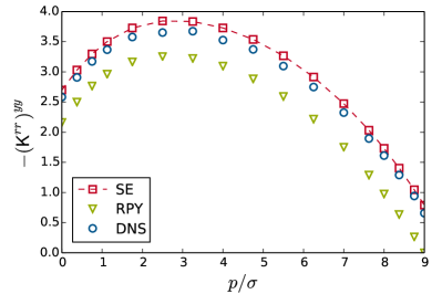
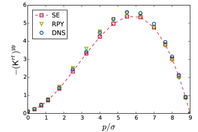
Figure 7: $yy$ friction coefficients for a helix of fixed length and number of turns, as a function of pitch $p/\sigma$ ($\sigma$ is the bead radius). (top) rotation-rotation and (bottom) rotation-translation friction tensor. The results obtained from DNS simulations are compared to the exact SE values, as well as those obtained using an RPY approximation.

Finally, to see in what way the structure of the helix will affect its motion, we consider the $yy$ components of the $\bm{\mathsf{K}}^{rt}$ and $\bm{\mathsf{K}}^{rr}$ friction matrices, as a function of the pitch distance $p$. As the pitch is increased and the helix starts to stretch, fluid flow between the turns of the helix will start to increase, while the cross sectional area of the particle ($xz$ plane) is reduced. The latter will increase the torque felt by the helix (as the particle must now drag the fluid along), while the former will tend to reduce it (by reducing the moment of inertia). These effects give rise to the behavior seen in fig 7, where the $\bm{\mathsf{K}}^{rr}$ coefficient shows a maximum at an intermediate pitch value $p/\sigma\simeq 3$. Similar behavior is observed for the $\bm{\mathsf{K}}^{rt}$ coefficient, although the maximum is obtained at a different pitch value $p/\sigma\simeq 6$, and the coupling between rotation and translation disappears for $p/\sigma=0$ and $p/\sigma=9$, as expected. For comparison purposes, we have also plotted the results obtained using the Ewald-summed RPY tensorBeenakker (1986) in fig 7. The agreement is surprisingly good for the $\bm{\mathsf{K}}^{tr}$ tensor, but a considerable discrepancy appears in the coefficients of the $\bm{\mathsf{K}}^{rr}$ tensor, as this RPY formulation does not include hydrodynamic effects arising from the particle rotation.

V Conclusions

We have extended the SP method to apply to arbitrary rigid bodies. For the moment, we have considered only particles constructed as a rigid agglomerate of (possibly overlapping) spherical beads, but alternative formulations are straightforward. We have verified the accuracy of our method by performing low Reynolds number DNS simulations to compute the single particle friction coefficients for a large variety of rigid bodies. Our results were compared with the exact solutions to the Stokes equation, showing excellent agreement in all cases. While there are several methods capable of performing these type of calculations, they impose a number of restrictions which can severely limit the type of systems to which they can be applied. Our method can capture the many-body hydrodynamic effects very accurately, and it is not restricted to zero Reynolds number flow or Newtonian host solvents. In future papers we will consider the lubrication effects of non-spherical particles (chains, rods, disks, tori, etc), as well as the dynamics at high Reynolds number and in the presence of a background flow fields.