Macroscopic quantum behaviour of periodic quantum systems

Abstract

In this paper we introduce a simple procedure for computing the macroscopic quantum behaviour of periodic quantum systems in the high energy regime. The macroscopic quantum coherence is ascribed to a one-particle state, not to a condensate of a many-particle system; and we are referring to a system of high energy but with few degrees of freedom. We show that, in the first order of approximation, the quantum probability distributions converge to its classical counterparts in a clear fashion, and that the interference effects are strongly suppressed. The harmonic oscillator provides a testing ground for these ideas and yields excellent results.

I Introduction

The superposition principle lies at the heart of quantum mechanics, and it is one of its features that most distinctly marks the departure from classical concepts Schlosshauer . Formally, the superposition principle is rooted in the linearity of the Hilbert space. A striking and inevitable counterintuitive consequence of this principle is the phenomenon of quantum interference. The simplest kind of interference is displayed in the famous double-slit experiments, first performed by Young in 1802 with light, then duplicated during the last century with all sorts of material particles.

At the macroscopic scale all happens as if, by a conspiracy of nature, the naked quantum is hidden, leaving us with an apparent world described consistently in a classical language Haroche . The question that naturally arises is if quantum effects can be observed at macroscopic level. A classical illustration of the conflict between the existence of quantum superpositions and our real-world experience (of observation and measurement) is the ”Schrödinger’s cat”, in which a cat is put in a quantum superposition of alive and dead states. A widely accepted explanation nowadays for the appearance of classical like features from an underlying quantum world is the environment induced decoherence approach Joos ; Zurek1 ; Zurek2 ; Giulini . According to this theory, coupling to a large number of degrees of freedom (the environment) results in a loss of quantum coherence which leads to emergent classicality.

In this paper we introduce a simple procedure to compute the high energy regime of a general density matrix for periodic quantum systems. We show that, in the first order of approximation, the quantum probability distribution converges to its classical counterpart in a clear fashion, and that the interference effects are strongly suppressed. The harmonic oscillator provides a testing ground for these ideas as we will illustrate. We demonstrates that the classical features emerges from its quantum description in the high energy regime. This problem has been considered before by Cabrera and Kiwi Cabrera . In this work, they use purely quantum-mechanical results to analyze (by inspection) the amplitude of the oscillations and the spatial autocorrelation function for large quantum numbers. They conclude that even for arbitrarily high quantum numbers, a superposition of (a few) eigenstates retains quantum effects. The originality of our paper lies in the fact that we propose a well-founded mathematical procedure for calculating the macroscopic manifestations of quantum behaviour.

The remainder of the paper is organized as follows. In Sec. II, we introduce the general procedure. The results for the harmonic oscillator are presented in Section III. Finally, some conclusions and remarks are given in Section IV.

II General procedure

It is generally accepted that the classical and quantum probability density functions for periodic systems approach each other in a locally averaged sense when the principal quantum number becomes large Liboff ; Auerbach ; Yoder ; Robinett , i.e.

$$\rho^{CL}\left(x\right)=\lim_{n\gg 1}\frac{1}{2\epsilon_{n}}\int_{x-\epsilon_{n}}^{x+\epsilon_{n}}\rho_{n}^{QM}\left(y\right)dy\,\text{,}$$ (1)

where the interval $\epsilon_{n}$ decreases with increasing the quantum number $n$. For a brief discussion of the meaning of the classical probability distribution see Ref.Robinett . The local averaging of the infinite square well potential is reported in Auerbach and Robinett . In most cases, Eq.(1) is very difficult to calculate analitically. We briefly review an alternative procedure to compute the local averages appearing Eq.(1) Bernal ; Martin . Supported by the harmonic analysis criteria, the authors write the classical and quantum distributions as a Fourier expansion,

$$\rho_{n}^{QM}\left(x\right) = \int f_{n}^{QM}\left(p\right)e^{i\frac{px}{\hbar}}dp,$$ (2)

$$\rho^{CL}\left(x\right) = \int f^{CL}\left(p\right)e^{i\frac{px}{\hbar}}dp,$$

where $f_{n}^{QM}\left(p\right)$ and $f^{CL}\left(p\right)$ are the Fourier coefficients of each expansion respectively. An immediate consequence of Eqs. (1) and (2) is that the Fourier coefficients have a similar behaviour for $n$ large,

$$f_{n}^{QM}\left(p\right)\sim f^{CL}\left(p\right).$$ (3)

Note that Planck’s constant keep a finite value, so $\hbar$-dependent corrections may arise in Eq.(3). This implies that even at macroscopic level the Heisenberg’s theorem works. Finally calculating the inverse Fourier transform of the asymptotic Fourier coefficients we obtain, at least in a first approximation, the classical probability density. Analytical results for the simplest quantum systems were reported Bernal ; Martin .

Now we focus on the general problem. Let us consider a physical system described completely by the Hamiltonian $\hat{H}$. Let $\left\{\left|\psi_{n}\right\rangle\right\}$ be an orthonormal basis of eigenvectors of $\hat{H}$ with eigenvalues $E_{n}$. If the initial state $\left|\Psi\left(0\right)\right\rangle$ has coefficients $c_{n}=\left\langle\psi_{n}|\Psi\left(0\right)\right\rangle$, then the state at a later time $t$, according to Schrödinger equation, is given by

$$\left|\Psi\left(t\right)\right\rangle=\sum_{n}c_{n}e^{-i\frac{E_{n}t}{\hbar}}\left|\psi_{n}\right\rangle.$$ (4)

The corresponding density matrix reads

$$\hat{\rho}\left(t\right)=\left|\Psi\left(t\right)\right\rangle\left\langle\Psi\left(t\right)\right|=\sum\limits_{n,m}c_{n}c_{m}^{\ast}e^{-i\frac{\left(E_{n}-E_{m}\right)t}{\hbar}}\left|\psi_{n}\right\rangle\left\langle\psi_{m}\right|.$$ (5)

The terms $m\neq n$ embody the quantum coherence between the different components $\left|\psi_{n}\right\rangle$. Accordingly, they are usually referred to as interference terms, or off-diagonal terms. Consequently, the expectation value of the arbitrary observable $\mathcal{O}$ is given by

$$\left\langle\mathcal{O}\right\rangle=Tr\left[\mathcal{O}\hat{\rho}\left(t\right)\right]=\sum\limits_{n,m}c_{n}c_{m}^{\ast}\mathcal{O}_{m,n}e^{-i\frac{\left(E_{n}-E_{m}\right)t}{\hbar}},$$ (6)

with $\mathcal{O}_{m,n}\equiv\left\langle\psi_{m}\right|\mathcal{O}\left|\psi_{n}\right\rangle$.

To explain our procedure, let us consider the coordinate representation of the matrix density. Its components are given by

$$\rho_{n,m}\left(x,t\right)=c_{n}c_{m}^{\ast}\tilde{\rho}_{n,m}\left(x\right)e^{-i\frac{\left(E_{n}-E_{m}\right)t}{\hbar}},$$ (7)

with $\tilde{\rho}_{n,m}\left(x\right)\equiv\psi_{n}\left(x\right)\psi_{m}^{\ast}\left(x\right)$. It is well known that space and time play fundamentally different roles in quantum mechanics: whereas position is represented by a hermitian operator, time is represented by a $c$-number Neumann . Then we study separately the roles of space and time in Eq.(7). We first consider the spacial behaviour.

It is well known that for periodic quantum systems, nodes are always present in the density matrix (by means of $\tilde{\rho}_{n,m}\left(x\right)$) for arbitrarily large quantum numbers, and thus the study of its macroscopic behaviour naturally implies an average process. To this end we extend the Fourier expansion in Eq.(2) to the spatial components of the matrix density (7),

$$\tilde{\rho}_{n,m}\left(x\right)=\int f_{n,m}\left(p\right)e^{i\frac{px}{\hbar}}dp,$$ (8)

where $f_{n,m}\left(p\right)$ are the Fourier coefficients of the expansion. Physically the Fourier coefficients $f_{n,m}\left(p\right)$ are the convolution $\phi_{n}\left(p\right)\ast\phi_{m}\left(p\right)$, where $\phi_{n}\left(p\right)$ is the wavefunction in momentum representation. Subsequently we consider the spacial asymptotic behaviour of the Fourier coefficients for large quantum numbers, and finally its inverse Fourier transform gives the desired macroscopic behaviour of $\tilde{\rho}_{n,m}\left(x\right)$. According to our macroscopic-world experience, the interference effects are completely suppressed. For instance, no one has ever seen a ball going through two directions at once Haroche . Therefore, the asymptotics of $\tilde{\rho}_{n,m}\left(x\right)$, for $n\neq m$, should be strongly suppressed.

We now study the temporal behaviour. We observe that Eq.(7) is an almost periodic function of the time (except for the diagonal terms), even for arbitrarily high energies. It is clear that the off-diagonal terms are a rapidly oscillating functions of the time when the energies differ significantly, and a slowly varying functions if the energies are close each other. This means that in the macroscopic regime becomes important only the interference between states with high energies $E_{n}$ and $E_{m}$, such that $\left|E_{n}-E_{m}\right|=E_{\upsilon}$ and $E_{\upsilon}\ll E_{n}$. Under these conditions the quantum-mechanical frequencies goes to its classical counterpart Lindenbaum , i.e.,

$$\omega_{\upsilon}^{QM}\equiv\frac{E_{n+\upsilon}-E_{n}}{\hbar}\approx 2\pi\upsilon\frac{\partial E_{n}}{\partial J}=\upsilon\omega^{CL}\text{,}$$ (9)

where we used the standard definition $\omega^{CL}\equiv 2\pi\frac{\partial E_{n}}{\partial J}$, where $J=nh$ is the action Goldstein .

We conclude this section with the final expression for the macroscopic density matrix in coordinate representation, i.e.,

$$\rho\left(x,t\right)\sim\sum\limits_{n,\upsilon}c_{n}c_{n-\upsilon}^{\ast}\tilde{\rho}_{n,n-\upsilon}\left(x\right)e^{-i\upsilon\omega^{CL}t}\text{.}$$ (10)

where we have included the spatial and temporal analysis described above. We observe that (10) is the Fourier expansion of a classical function, which can be inmediately identified with the classical probability distribution $\rho^{CL}\left[x\left(t\right)\right]$. Note that the long-time behavior of $\rho\left(x,t\right)$ converges towards $\sum\limits_{n}\left|c_{n}\right|^{2}\tilde{\rho}_{n,n}\left(x\right)$, in agreement with the classical result. We point out that in our work the macroscopic quantum coherence is ascribed to a one-particle state, not to a condensate of a many-particle system. We are referring to a system of high energy, but with few degrees of freedom. In the next section we present analytical results for the harmonic oscillator.

III Macroscopic density matrix of the harmonic oscillator

The harmonic oscillator provides a testing ground for these ideas as we now illustrate. We first consider again the spacial behaviour. The energy eigenfunctions and eigenvalues of the corresponding Schrödinger equation are well known. The quantized energies are given by

$$E_{n}=\hbar\omega\left(n+\frac{1}{2}\right)$$ (11)

with $n\in\mathbb{Z}^{+}$, while the stationary states can be written as follows

$$\psi_{n}\left(x\right)=\sqrt[4]{\frac{\alpha}{\pi}}\frac{1}{\sqrt{2^{n}n!}}H_{n}\left(\sqrt{\alpha}x\right)e^{-\frac{\alpha x^{2}}{2}}$$ (12)

where $\alpha=\frac{m\omega}{\hbar}$. The spatial components of the matrix density are given by

$$\tilde{\rho}_{n,m}\left(x\right)=\sqrt{\frac{\alpha}{\pi}}\frac{1}{\sqrt{2^{n}n!2^{m}m!}}H_{n}\left(\sqrt{\alpha}x\right)H_{m}\left(\sqrt{\alpha}x\right)e^{-\alpha x^{2}}\text{.}$$ (13)

Figure 1 illustrates the spatial components $\tilde{\rho}_{n,m}\left(x\right)$ for different values of $n$ and $m$. In Figs. 1(a), 1(b) and 1(c) we first consider the smooth oscillatory quantum regime for $n=1$ and $m=1,10,~{}20$, respectively. When increasing the quantum numbers, $\tilde{\rho}_{n,m}\left(x\right)$ becomes a rapidly oscillatory functions around the $x$-axis. This is illustrated in Figs. 1(d), 1(e) and 1(f) for $n=100$ and $m=100,125,150$, respectively. As we anticipated, nodes are always present for arbitrarily large quantum numbers. Note that the number of nodes increase with decreasing the difference $n-m$. It is clear that, after the local averaging process, the off-diagonal components will be strongly suppresed compared with the diagonal terms. Now we focus on applying the procedure presented in Sec.I.

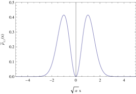
(a)

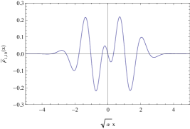
(b)

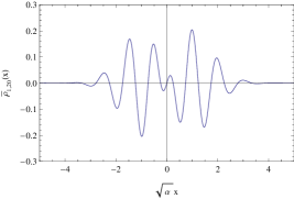
(c)

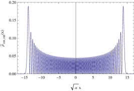
(d)

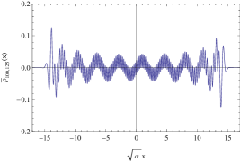
(e)

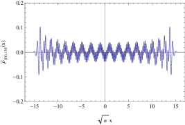
(f)

Figure 1: Spatial behaviour of $\bar{\rho}_{n,m}\left(x\right)\equiv\frac{\tilde{\rho}_{n,m}\left(x\right)}{\sqrt{\alpha}}$.  Graphs (a), (b) and (c) corresponds to $n=1$ and $m=1,10,~{}20$, respectively. The high energy regime is illustrated in graphs (d), (e) and (f) for $n=100$ and $m=100,125,150$, respectively.

We first calculate the Fourier coefficients appearing in Eq.(8). The corresponding inverse Fourier transform is reported in many handbooks of mathematical functions Abramowitz ; Gradshteyn :

$$f_{n,m}\left(p\right)=\left(-i\right)^{n-m}\sqrt{\frac{m!}{n!}}e^{-\frac{\xi_{0}^{2}}{2}}\xi_{0}^{n-m}L_{m}^{n-m}\left(\xi_{0}^{2}\right)$$ (14)

where $n\geq m$, $\xi_{0}\equiv\frac{p}{\sqrt{2m\omega\hbar}}$ and $L_{m}^{n-m}$ is an associated Laguerre polynomial. In this expression it can be seen that the correlation between two wave functions increases as the difference $n-m$ decrease.

The asymptotic behaviour of $f_{n,m}\left(p\right)$, for $n$ and $m$ large, is also well known. Szegö finds the following iterative relation for $n$ large Szego :

$$u\left(x\right) = e^{-\frac{x^{2}}{2}}x^{\upsilon}L_{n}^{\upsilon}\left(x^{2}\right)\sim\frac{\Gamma\left(n+\upsilon+1\right)}{N^{\frac{\upsilon}{2}}n!}J_{\upsilon}\left(2\sqrt{N}x\right)-\frac{\pi}{2}\times$$

$$\int_{0}^{x}y^{3}u\left(y\right)\left[J_{\upsilon}\left(2\sqrt{N}x\right)Y_{\upsilon}\left(2\sqrt{N}y\right)-Y_{\upsilon}\left(2\sqrt{N}x\right)J_{\upsilon}\left(2\sqrt{N}y\right)\right]dy$$

where $J_{\upsilon}$ and $Y_{\upsilon}$ are the usual Bessel functions of the first and second kind respectively, and $N=n+\frac{\upsilon+1}{2}$. Szegö also shows that the iteration terms are strongly suppressed compared with the first order of approximation in the limit $N\rightarrow\infty$. In this paper we will consider only the first order of approximation, however the higher orders of approximation follows immediately from Eq.(III). The asymptotic behaviour of the Fourier coefficients is then

$$f_{n,n-\upsilon}\left(p\right)\sim\frac{\left(-i\right)^{\upsilon}}{\left(1-\frac{\upsilon-1}{2n}\right)^{{}^{\frac{\upsilon}{2}}}}J_{\upsilon}\left(2\sqrt{N}\xi_{0}\right)$$ (16)

with $N=n-\frac{\upsilon-1}{2}$ and $\upsilon=n-m$, such that $n\gg\upsilon\geq 0$. In Eq.(16) we have used the approximation $\frac{n!}{m!}\sim n^{\upsilon}$. From Eq.(16) it follows that, in the asymptotic Fourier coefficients matrix, the order of the Bessel function increases as we move away from the main diagonal. For example, in the main diagonal we have $J_{0}\left(2\sqrt{n+\frac{1}{2}}\xi_{0}\right)$, in the secondary diagonals we have firstly $-iJ_{1}\left(2\sqrt{n}\xi_{0}\right)$, secondly $-\left(1-\frac{1}{2n}\right)^{-\frac{1}{{}^{{}^{2}}}}J_{2}\left(2\sqrt{n+\frac{1}{2}}\xi_{0}\right)$, and so on. Physically this means that in the high energy regime the interference between two states becomes important when its energies are close each other, as anticipated.

Finally the macroscopic behaviour of $\tilde{\rho}_{n,n-\upsilon}\left(x\right)$ is obtained by substituting the Eq.(16) into Eq.(8) and calculating the resulting Fourier transform. In Refs.Erdelyi and Kammler is reported the Fourier transformation of Bessel functions. Our final expression for the asymptotic behaviour of $\tilde{\rho}_{n,n-\upsilon}\left(x\right)$ for large quantum numbers is then

$$\tilde{\rho}_{n,n-\upsilon}\left(x\right)\sim\frac{1}{\left(1-\frac{\upsilon-1}{2n}\right)^{{}^{\frac{\upsilon}{2}}}}\frac{T_{\upsilon}\left(\frac{x}{\chi_{n,n-\upsilon}}\right)}{\pi\sqrt{\chi_{n,n-\upsilon}^{2}-x^{2}}}\mathrm{Rect}\left(\frac{x}{2\chi_{n,n-\upsilon}}\right)$$ (17)

where $\chi_{n,n-\upsilon}\equiv\sqrt{\frac{2N\hbar}{m\omega}}$, $T_{\upsilon}$ is the Chebyshev polynomial of the first kind and $\mathrm{{\mathrm{Rect}}}$ is the rectangular function. Note that the rectangular function restricts the domain of (17) to $x\in\left[-\chi_{n,n-\upsilon},\chi_{n,n-\upsilon}\right]$.

We observe that the diagonal terms in (17) are simply

$$\tilde{\rho}_{n,n}\left(x\right)\sim\frac{1}{\pi\sqrt{x_{n}^{2}-x^{2}}}\mathrm{{\mathrm{Rect}}}\left(\frac{x}{2x_{0}}\right)\text{,}$$ (18)

with $x_{n}\equiv\chi_{n,n}=\sqrt{\frac{2\left(n+\frac{1}{2}\right)\hbar}{m\omega}}$. Note that $\tilde{\rho}_{n,n}\left(x\right)$ coincides with the probability density of a classical harmonic oscillator with amplitude $x_{n}$. Rearranging the expression for $\chi_{n,n}$ we obtain $\frac{1}{2}m\omega^{2}x_{n}^{2}=\hbar\omega\left(n+\frac{1}{2}\right)$, which is the well known expression for the classical energy. Therefore we have shown that the classical features (e.g. amplitude, energy, probability distribution and the confinement effect) naturally emerge as the first order of approximation of quantum mechanics in the high energy regime. When considering higher orders of approximation in (18) we observe macroscopic quantum behaviour. For example, a residual oscillatory behaviour (in all space) is retained in $\tilde{\rho}_{n,n}\left(x\right)$ even for arbitrarily high quantum number $n$ Bernal . This is because $\hbar$ keeps a finite value, and thus the Heisenberg’s theorem still works. The exact classical result is recovered if we take $\hbar\rightarrow 0$, however $\hbar$ is a fundamental constant of nature whose numerical value although small is not zero.

The exact classical limit requires the off-diagonal terms equal to zero (means no interference), however according to our result (17) this is never attained. In figures 2 we present the asymptotic behaviour of $\tilde{\rho}_{n,n-\upsilon}\left(x\right)$ for $n=10000$ and different values of $\upsilon$. Figs. 2(a) and 2(b) depict the interference between neighboring states with $\upsilon=1,2$ respectively, while in figs. 2(c) and 2(d) we consider states with $\upsilon=50,100$ respectively. Note that in all cases, although the interference effect is very small (less than $0.01$) is not zero. Also it can be seen that the nodes increase with increasing $\upsilon$, so that the expectation values $\left\langle\psi_{m}\right|\mathcal{O}\left|\psi_{n}\right\rangle$ of a smooth function $\mathcal{O}\left(x\right)$ converge more rapidly to zero for $\upsilon$ large. This means that at high energies the interference becomes important only for neighboring states.

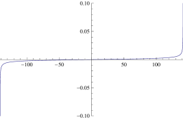
(a)

(b)

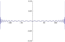
(c)

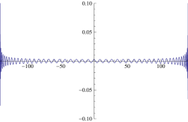
(d)

Figure 2: Asymptotic spatial behaviour of $\bar{\rho}_{n,m}\left(x\right)\equiv\frac{\tilde{\rho}_{n,m}\left(x\right)}{\sqrt{\alpha}}$ for $n=10000$. Graphs (a) and (b) depict the interference between neighboring states with $\upsilon=1,2,$ respectively, while in graphs (c) and (d) we consider states with $\upsilon=50,100,$ respectively.

Regarding to the temporal behaviour, from Eq.(7) it follows that the off-diagonal temporal terms in the matrix density are simply $e^{-i\upsilon\omega t}$, were we used (11). We observe that the frequency of the temporal oscillations increase as we move away from the main diagonal. In this case the high energy temporal behaviour is exactly the same as its low energy counterpart (with the same $\upsilon$). In the macroscopic regime $\upsilon\ll n$ therefore $e^{-i\upsilon\omega t}$ is a slowly varying function.

To complete this section we write an asymptotic expression for the expectation value of an arbitrary observable $\mathcal{O}$. According to our results $\left\langle\mathcal{O}\right\rangle$ will be, at first order of approximation, the classical expectation value $\left\langle\mathcal{O}\right\rangle^{CL}$ plus corrections coming from the possible interferece between states, i.e.

$$\left\langle\mathcal{O}\right\rangle\sim\left\langle\mathcal{O}\right\rangle^{CL}+\sum\limits_{n,\upsilon}\frac{c_{n}c_{n-\upsilon}^{\ast}e^{-i\upsilon\omega t}}{\left(1-\frac{\upsilon-1}{2n}\right)^{{}^{\frac{\upsilon}{2}}}}\int_{-1}^{+1}\mathcal{O}\left(\chi_{n,n-\upsilon}\xi\right)\frac{T_{\upsilon}\left(\xi\right)}{\pi\sqrt{1-\xi^{2}}}d\xi,$$ (19)

where $\left\langle\mathcal{O}\right\rangle^{CL}=\sum\limits_{n}\left|c_{n}\right|^{2}\int\mathcal{O}\left(x\right)\tilde{\rho}_{n,n}\left(x\right).$ We can also evaluate higher orders of approximation in a simple fashion Szego , however these are strongly suppressed compared with Eq.(19). In practice only a few number of terms are important in the summation. Because the properties of Chebyshev polynomials, if $\mathcal{O}\left(x\right)$ is a polynomial function of order $k$, then the integral in Eq.(19) vanishes for $k>\upsilon$ Abramowitz . Therefore $\left\langle x\right\rangle$ and $\left\langle x^{2}\right\rangle$ requires only $\upsilon=1,2$, respectively. We point out that the ergodic behaviour of Eq.(19) yields the correct classical expectation value.

IV Final remarks

It is well known that the concepts of classical and macroscopic systems are distinct, as the existence of macroscopic quantum phenomena (such as superconductivity) demonstrates, but the behaviour of most macroscopic systems can be described by classical theories Ballentine . In this paper we have shown that quantum mechanics is applicable in every scale of nature, and the macroscopic regime emerge as a consequence of its high energy behaviour. Quantum effects remains at this level (called macroscopic quantum behaviour), as the interference between quantum states. It would be interesting to test these effects with real quantum systems approaching the microscopic-macroscopic boundary, as Rydberg atoms or neutron interferometry for example. At higher energies these macroscopic quantum effects are so strongly suppressed that it is impossible to detect, leaving us with an apparent world described consistently in a classical language. With the appropriate experimental devices such effects should be observed even in our real-world experience, however nowadays it is impossible.

Technical difficulties in the calculation of the Kepler problem are greater than in the simple case which we have treated here, however we can definetly foresee that our procedure gives its correct macroscopic behaviour. Even though our approach gives the correct classical results for periodic quantum systems, it is far from the general solution to the classical limit problem. Several other questions remain to be resolved as the study of unbound systems and entanglement, but is not clear in the framework adopted here. The environment induced decoherence approach successfully resolves these problems.

Based in our results, in our future research we intend to concentrate on the definition of the classical regime, which is of considerable importance in the study of quantum chaos.

B. Buck and C. V. Sukumar, Phys. Lett. 83A, 132 (1981).

American Journal of Physics – May 2006 – Volume 74, Issue 5, pp. 404

References

- (1) Schlosshauer, M., Decoherence and the Quantum-to-Classical Transition, 1st Edition. Springer, Berlin/Heidelberg, 2007.
- (2) Serge Haroche and Jean-Michel Raimond, Exploring the Quantum. Atoms, Cavities, and Photons, Oxford University Press, New York, 2006.
- (3) Joos, E. and Zeh, H. D., Z. Phys. B 59, 223 (1985).
- (4) Zurek, W. H., Phys. Today 44, 36 (1991).
- (5) Zurek, W. H. Rev. Mod. Phys. 75, 715 (2003).
- (6) Giulini, D., Joos, E., Kiefer, C., Kupsch, J., Stamatescu, I. O. and Zeh, H. D. Decoherence and the appearance of the classical world in quantum theory, Springer, Berlin, 1996.
- (7) G. G. Cabrera and M. Kiwi, Phys. Rev. A 36, 2995–2998 (1987).
- (8) R. Liboff, Introductory Quantum Mechanics, 4th ed., Addison-Wesley, Boston, 2002.
- (9) Luis de la Peña, Introducción a la Mecánica Cuántica, México: FCE, UNAM, 2006.
- (10) G. Yoder, Am. J. Phys., Vol. 74, No. 5, (2006).
- (11) R. W. Robinett, Am. J. Phys., Vol. 63, No. 9, (1995).
- (12) J. Bernal, A. Martín-Ruiz and J. García-Melgarejo, Journal of Modern Physics, Vol. 4, No. 1, (2013).
- (13) A. Martín-Ruiz, J. Bernal, A. Frank and A. Carbajal-Dominguez, Journal of Modern Physics, Vol. 4, No. 6, (2013).
- (14) J. von Neumann, Mathematical Foundations of Quantum Mechanics (1932). Translated by R. T. Beyer Princeton University Press, Princeton, NJ, 1955.
- (15) Samuel D. Lindenbaum, Lecture Notes on Quantum Mechanics, World Scientific Pub Co Inc (June 1999)
- (16) Goldstein H., Poole C. P. and Safko J. P., Classical Mechanics, Addison-Wesley, San Francisco CA, 2002.
- (17) M. Abramowitz and I. Stegun, Handbook of Mathematical Functions: with Formulas, Graphs, and Mathematical Tables, Dover Publications, New York, 1965.
- (18) I. S. Gradshteyn and I. M. Ryzhik. Table of Integrals, Series, and Products. Edited by A. Jeffrey and D. Zwillinger. Academic Press, New York, 4th edition, 1994.
- (19) G. Szegö, Orthogonal Polynomials, American Mathematical Society, Providence, 1939.
- (20) Erdélyi, Arthur, Tables of Integral Transforms 1, New Your: McGraw-Hill, 1954.
- (21) Kammler, David, A First Course in Fourier Analysis, Prentice Hall, 2000.
- (22) L. E. Ballentine, Quantum mechanics: a modern development, World Scientific, New York, 1998.