Bound states of the one-dimensional Dirac equation
for scalar and vector double square-well potentials

Abstract

We have analytically studied bound states of the one-dimensional Dirac equation for scalar and vector double square-well potentials (DSPs), by using the transfer-matrix method. Detailed numerical calculations of the eigenvalue, wave function and density probability have been performed for the three cases: (1) vector DSP only, (2) scalar DSP only, and (3) scalar and vector DSPs with equal magnitudes. We discuss the difference and similarity among results of the cases (1)-(3) in the Dirac equation and that in the Schrödinger equation. Motion of a wave packet is calculated for a study on quantum tunneling through the central barrier in the DSP.

I Introduction

The basic physics of relativistic quantum mechanics was formulated in the Dirac equation, which elucidates the origin of spin 1/2 of an electron and predicts the existence of an antiparticle (a positron) Greiner81 . The Dirac equation has been applied not only to realistic models like hydrogen atom but also to pedagogical models which play important roles in understanding the properties of the Dirac equation. The Dirac equation for step and square potentials has been investigated in connection to the Klein paradox Thomson91 ; Nitta99 ; Krekora04 ; Le06 ; Bosanac07 . Square-well potentials with finite and infinite depths have been studied in Refs. Coulter71 ; Gumbs86 ; Coutinho88 ; Alberto96 ; Alhaidari11 ; Ying04 . The double square-well potential (DSP) consisting of the confining potential and the central potential is more difficult than the single square-well potential Coulter71 ; Gumbs86 ; Coutinho88 ; Alberto96 ; Alhaidari11 ; Ying04 . Indeed applications of the Dirac equation to the DSP have not been reported as far as we are aware of Note1 . The DSP is a simplified model for an appropriate and realistic description of a continuous double-well potential. Extensive investigations within the nonrelativistic treatment of the Schrödinger equation have been made for double-well systems where numerous quantum phenomena have been realized (for a recent review on double-well systems, see Ref. Thorwart01 ). The Schrödinger equation for the DSP with the infinite confining potential is manageable and treated in the undergraduate text, whereas the DSP with the finite confining potential has been investigated only in several studies Lopez06 ; Acus11 ; Tserkis13 . One of advantages of the DSP is to provide us with exact analytic expressions for eigenstates and wave functions. In the relativistic quantum theory, two types of vector ($V(x)$) and scalar ($S(x)$) potentials have been adopted. In previous studies on the single square-well potential, the vector potential was adopted in Refs. Coulter71 ; Gumbs86 ; Coutinho88 ; Alhaidari11 ; Ying04 while the scalar potential was employed in Refs. Coutinho88 ; Alberto96 . The purpose of this paper is to make a detailed study on the Dirac equation for scalar and vector DSPs and to make a comparison between results of the Dirac equation and the Schrödinger equation. Such a study is expected to be essential and inevitable for a deeper understanding of relativistic quantum double-well systems.

The paper is organized as follows. In Sec. II, we obtain analytic expressions for eigenvalues and wave functions of bound states in the Dirac equation for scalar and vector DSPs, by using the transfer-matrix method. In Sec. III, the transcendental complex equation for the eigenvalue is numerically solved and bound-state wave functions are obtained for three cases: (1) the vector DSP only (VDSP: $S(x)=0$), (2) the scalar DSP only (SDSP: $V(x)=0$), and (3) equal scalar and vector DSPs (EDSP: $S(x)=V(x)$). In Sec. IV, eigenvalues in the Dirac equation are compared to those obtained in the Schrödinger equation. Motion of a wave packet is investigated for a study on the quantum tunneling through the central barrier in the DSP. Sec. V is devoted to our conclusion. In the Appendix the transfer-matrix method is applied to the Schrödinger equation for the DSP.

II Dirac equation for the double square-well potential

II.1 Transfer-matrix formulation

We will obtain the bound-state solution of the stationary one-dimensional Dirac equation for the DSP. Among conceivable, equivalent expressions for the Dirac equation, we employ the $(1+1)$-dimensional representation

$$\left[c\>\sigma_{x}\left(-i\hbar\frac{\partial}{\partial x}\right)+\sigma_{z}\left[mc^{2}+S(x)\right]\right]\Psi(x) = \left[E-V(x)\right]\>\Psi(x),$$ (1)

with

$$\Psi(x) = \left({\begin{array}[]{*{20}c}\psi_{+}(x)\\ \psi_{-}(x)\\ \end{array}}\right),$$ (4)

where $\psi_{\pm}(x)$ signify elements of two-dimensional spinor of $\Psi(x)$, $\sigma_{x}$ and $\sigma_{z}$ are Pauli matrices, $S(x)$ and $V(x)$ express scalar and vector potentials, respectively, $E$ denotes the stationary energy, $m$ is rest mass of a particle with spin 1/2, and $c$ is the light velocity. Two component of $\psi_{+}(x)$ and $\psi_{-}(x)$ satisfy

$$[mc^{2}+V(x)+S(x)]\psi_{+}(x)-i\hbar c\frac{d}{dx}\psi_{-}(x) = E\psi_{+}(x),$$ (5)

$$-i\hbar c\frac{d}{dx}\psi_{+}(x)+[-mc^{2}+V(x)-S(x)]\psi_{-}(x) = E\psi_{-}(x).$$ (6)

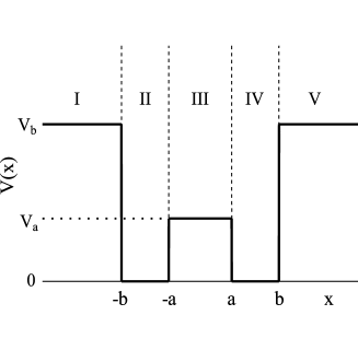
Figure 1: Schematic vector DSP, $V(x)$, given by Eqs. (12) (bold solid lines), the $x$ axis being divided into five regions I-V separated by dashed lines. The scalar DSP, $S(x)$, is given if we read $V_{a}\rightarrow S_{a}$ and $V_{b}\rightarrow S_{b}$.

We consider the one-dimensional vector potential $V(x)$ expressed by

$$V(x) = \left\{\begin{array}[]{ll}V_{b}&\mbox{for $x\leq-b$ \hskip 34.14322pt (region I)},\\ 0&\mbox{for $-b<x\leq-a$ \hskip 5.69046pt (region II)},\\ V_{a}&\mbox{for $-a<x\leq a$ \hskip 14.22636pt (region III)},\\ 0&\mbox{for $a<x\leq b$ \hskip 28.45274pt (region IV)},\\ V_{b}&\mbox{for $x>b$ \hskip 42.67912pt (region V)},\end{array}\right.$$ (12)

with $V_{b}\geq 0$ and $0\leq V_{a}\leq V_{b}$. Here the $x$ axis is divided into five spatial regions: (I) $x\leq-b$, (II) $-b\leq x\leq-a$, (III) $-a<x\leq a$, (IV) $a<x\leq b$, and (V) $x>b$; $V_{b}$ expresses the confining potential in the regions I and V; $V_{a}$ denotes central barrier potential in the region III (Fig. 1).

As for the scalar potential $S(x)$, we consider

$$S(x) = \left\{\begin{array}[]{ll}S_{b}&\mbox{for $x\leq-b$ \hskip 34.14322pt (region I)},\\ 0&\mbox{for $-b<x\leq-a$ \hskip 5.69046pt (region II)},\\ S_{a}&\mbox{for $-a<x\leq a$ \hskip 14.22636pt (region III)},\\ 0&\mbox{for $a<x\leq b$ \hskip 28.45274pt (region IV)},\\ S_{b}&\mbox{for $x>b$ \hskip 42.67912pt (region V)},\end{array}\right.$$ (18)

with $S_{b}\geq 0$ and $0\leq S_{a}\leq S_{b}$ (read $V_{a}\rightarrow S_{a}$ and $V_{b}\rightarrow S_{b}$ in Fig. 1). The adopted scalar and vector DSPs are symmetric with respect to the origin. In the limit of $V_{a}=S_{a}=0$, $a=0$, or $a=b$, the double square-well potential reduces to the single one.

Wave functions in five regions I-V may be expressed by

$$\Psi_{I}(x) = A_{1}\left({\begin{array}[]{*{20}c}1\\ \beta\\ \end{array}}\right)e^{iqx}+B_{1}\left({\begin{array}[]{*{20}c}1\\ {-\beta}\\ \end{array}}\right)e^{-iqx}\hskip 28.45274pt\mbox{for $x<-b$},$$ (23)

$$\Psi_{II}(x) = A_{2}\left({\begin{array}[]{*{20}c}1\\ \alpha\\ \end{array}}\right)e^{ikx}+B_{2}\left({\begin{array}[]{*{20}c}1\\ {-\alpha}\\ \end{array}}\right)e^{-ikx}\hskip 28.45274pt\mbox{for $-b<x<-a$},$$ (28)

$$\Psi_{III}(x) = A_{3}\left({\begin{array}[]{*{20}c}1\\ \gamma\\ \end{array}}\right)e^{ipx}+B_{3}\left({\begin{array}[]{*{20}c}1\\ {-\gamma}\\ \end{array}}\right)e^{-ipx}\hskip 28.45274pt\mbox{for $-a<x<a$},$$ (33)

$$\Psi_{IV}(x) = A_{4}\left({\begin{array}[]{*{20}c}1\\ \alpha\\ \end{array}}\right)e^{ikx}+B_{4}\left({\begin{array}[]{*{20}c}1\\ {-\alpha}\\ \end{array}}\right)e^{-ikx}\hskip 28.45274pt\mbox{for $a<x<b$},$$ (38)

$$\Psi_{V}(x) = A_{5}\left({\begin{array}[]{*{20}c}1\\ \beta\\ \end{array}}\right)e^{iqx}+B_{5}\left({\begin{array}[]{*{20}c}1\\ {-\beta}\\ \end{array}}\right)e^{-iqx}\hskip 28.45274pt\mbox{for $x<-a$},$$ (43)

with

$$k = \frac{\sqrt{E^{2}-m^{2}c^{4}}}{\hbar c},$$ (44)

$$p = \frac{\sqrt{(E+mc^{2}-V_{a}+S_{a})(E-mc^{2}-V_{a}-S_{a})}}{\hbar c},$$ (45)

$$q = \frac{\sqrt{(E+mc^{2}-V_{b}+S_{b})(E-mc^{2}-V_{b}-S_{b})}}{\hbar c},$$ (46)

$$\alpha = \frac{\hbar ck}{E+mc^{2}},$$ (47)

$$\beta = \frac{\hbar cq}{E+mc^{2}-V_{b}+S_{b}},$$ (48)

$$\gamma = \frac{\hbar cp}{E+mc^{2}-V_{a}+S_{a}},$$ (49)

where $\sqrt{z}$ signifies the square root of a complex $z$: for a real $z$, $\sqrt{z}=z^{1/2}\>\Theta(z)+i\>(-z)^{1/2}\>\Theta(-z)$ with the Heaviside function $\Theta(z)$.

Matching conditions of wave functions at boundaries at $x=\pm b$ and $x=\pm a$ yield

$$\left({\begin{array}[]{*{20}c}{e^{-iqb}}&{e^{iqb}}\\ {\beta\>e^{-iqb}}&{-\beta\>e^{iqb}}\\ \end{array}}\right)\left({\begin{array}[]{*{20}c}{A_{1}}\\ {B_{1}}\\ \end{array}}\right) = \left({\begin{array}[]{*{20}c}{e^{-ikb}}&{e^{ikb}}\\ {\alpha\>e^{-ikb}}&{-\alpha\>e^{ikb}}\\ \end{array}}\right)\left({\begin{array}[]{*{20}c}{A_{2}}\\ {B_{2}}\\ \end{array}}\right),$$ (58)

$$\left({\begin{array}[]{*{20}c}{e^{-ika}}&{e^{ika}}\\ {\alpha\>e^{-ika}}&{-\alpha\>e^{ika}}\\ \end{array}}\right)\left({\begin{array}[]{*{20}c}{A_{2}}\\ {B_{2}}\\ \end{array}}\right) = \left({\begin{array}[]{*{20}c}{e^{-ipa}}&{e^{ipa}}\\ {\gamma\>e^{-ipa}}&{-\gamma\>e^{ipa}}\\ \end{array}}\right)\left({\begin{array}[]{*{20}c}{A_{3}}\\ {B_{3}}\\ \end{array}}\right),$$ (67)

$$\left({\begin{array}[]{*{20}c}{e^{ipa}}&{e^{-ipa}}\\ {\gamma\>e^{ipa}}&{-\gamma\>e^{-ipa}}\\ \end{array}}\right)\left({\begin{array}[]{*{20}c}{A_{3}}\\ {B_{3}}\\ \end{array}}\right) = \left({\begin{array}[]{*{20}c}{e^{ika}}&{e^{-ika}}\\ {\alpha\>e^{ika}}&{-\alpha\>e^{-ika}}\\ \end{array}}\right)\left({\begin{array}[]{*{20}c}{A_{4}}\\ {B_{4}}\\ \end{array}}\right),$$ (76)

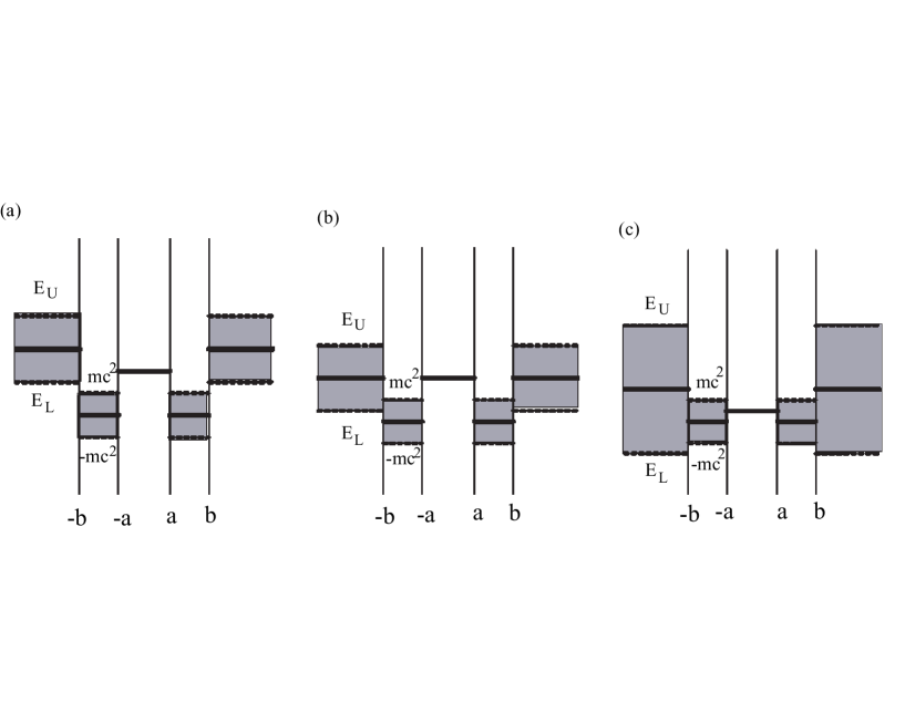
Figure 2: (Color online) Critical energy levels for (a) $V_{b}-S_{b}\geq 2mc^{2}$, (b) $0\leq V_{b}-S_{b}<2mc^{2}$, and (c) $V_{b}-S_{b}<0$ ($E_{U}=V_{b}+S_{b}+mc^{2}$, $E_{L}=V_{b}-S_{b}-mc^{2}$), wave vectors of $k$ and $p$ being purely imaginary in dark areas (see text).

$$\left({\begin{array}[]{*{20}c}{e^{ikb}}&{e^{-ikb}}\\ {\alpha\>e^{ikb}}&{-\alpha\>e^{-ikb}}\\ \end{array}}\right)\left({\begin{array}[]{*{20}c}{A_{4}}\\ {B_{4}}\\ \end{array}}\right) = \left({\begin{array}[]{*{20}c}{e^{iqb}}&{e^{-iqb}}\\ {\beta\>e^{ipb}}&{-\beta\>e^{-ipb}}\\ \end{array}}\right)\left({\begin{array}[]{*{20}c}{A_{5}}\\ {B_{5}}\\ \end{array}}\right).$$ (85)

By matrix calculation, we obtain

$$\left({\begin{array}[]{*{20}c}{A_{i}}\\ {B_{i}}\\ \end{array}}\right) = {\sf M}_{i\>i+1}\left({\begin{array}[]{*{20}c}{A_{i+1}}\\ {B_{i+1}}\\ \end{array}}\right)\hskip 28.45274pt\mbox{for $i=1-4$},$$ (90)

yielding

$$\left({\begin{array}[]{*{20}c}{A_{1}}\\ {B_{1}}\\ \end{array}}\right) = {\sf T}\left({\begin{array}[]{*{20}c}{A_{5}}\\ {B_{5}}\\ \end{array}}\right)=\left({\begin{array}[]{*{20}c}{T_{11}}&{T_{12}}\\ {T_{21}}&{T_{22}}\\ \end{array}}\right)\left({\begin{array}[]{*{20}c}{A_{5}}\\ {B_{5}}\\ \end{array}}\right),$$ (99)

where the transfer matrix ${\sf T}$ given by ${\sf T}={\sf M}_{1\>2}\>{\sf M}_{2\>3}\>{\sf M}_{3\>4}\>{\sf M}_{4\>5}$ includes information on the properties of a particle under consideration.

II.2 Bound-state condition

In order to obtain eigenvalues of a bounded particle, we set $A_{1}=B_{5}=0$ in Eq. (99), which is satisfied by $T_{11}=0$. After some matrix manipulations, we obtain the eigenvalue condition given by

$$T_{11} = \frac{e^{2iqb}}{16\alpha^{2}\beta\gamma}\{(\alpha+\gamma)^{2}\left[(\alpha+\beta)^{2}\>e^{2i[k(a-b)-pa]}-(\alpha-\beta)^{2}\>e^{-2i[k(a-b)-pa]}\right]$$ (100)

$$+ (\alpha-\gamma)^{2}\left[(\alpha-\beta)^{2}\>e^{-2i[k(a-b)+pa]}-(\alpha+\beta)^{2}\>e^{2i[k(a-b)+pa]}\right]$$

$$+ 2(\alpha^{2}-\beta^{2})(\alpha^{2}-\gamma^{2})\left[\>e^{2ipa}-e^{-2ipa}\right]\}=0.$$

Equation (100) determines both even- and odd-parity solutions.

It is necessary to solve the transcendental complex equation given by Eq. (100) in order to obtain eigenvalues of a bounded particle. Once an eigenvalue $E=E_{n}$ for an index $n$ ($=1,2,\cdots$) is obtained, we may successively determine coefficients of $A_{i}$ and $B_{i}$ ($i=2-4$) and $B_{1}$, starting from assumed coefficients of $A_{5}=C$ and $B_{5}=0$ by using Eq. (90). The magnitude of the assumed $C$ is determined by the normalization condition for the density probability $\rho(x)$ given by

$$\int_{-\infty}^{\infty}\rho(x)\>dx = 1,$$ (101)

with

$$\rho(x) = |\psi_{+}(x)|^{2}+|\psi_{-}(x)|^{2},$$ (102)

which may be analytically evaluated.

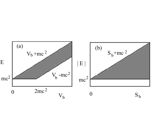
Figure 3: (Color online) Energy ranges of bound states for (a) the VDSP [Eq. (108)] and (b) the SDSP [Eq. (109)], bound states existing in shaded regions. The energy range for EDSP is expressed by (b) if we read $S_{b}+mc^{2}\rightarrow 2S_{b}+mc^{2}$ [Eq. (110)].

II.3 Bound-state energy range

We examine the energy range for bound states. Depending on magnitudes of $V_{b}-S_{b}$ and $mc^{2}$, the properties of wave vectors $k$ and $q$ change in the three cases: (A) $V_{b}-S_{b}\geq 2mc^{2}$, (B) $0\leq V_{b}-S_{b}<2mc^{2}$ and (C) $V_{b}-S_{b}<0$, as shown in Figs. 2(a), 2(b) and 2(c), respectively, where $k$ and $p$ are purely imaginary in dark areas. Bound states exist when $k$ is real but $q$ is purely imaginary which lead to plane waves in regions II and IV and evanescent waves in regions I and V. When the above condition is satisfied, bound states exist independently of whether the wave vector $p$ in the region III is real or imaginary. We obtain such energy regions for bound states given by

$$E_{L} < E<E_{U}\hskip 119.50148pt\mbox{for case A ($V_{b}-S_{b}\geq 2mc^{2}$)},$$ (103)

$$mc^{2} < E<E_{U}\hskip 119.50148pt\mbox{for case B ($0\leq V_{b}-S_{b}<2mc^{2}$)},$$ (104)

$$mc^{2} < E<E_{U}\hskip 5.69046pt{\rm or}\hskip 5.69046ptE_{L}<E<-mc^{2}\hskip 14.22636pt\mbox{for case C ($V_{b}-S_{b}<0$)},$$ (105)

where

$$E_{U} = V_{b}+S_{b}+mc^{2},$$ (106)

$$E_{L} = V_{b}-S_{b}-mc^{2}.$$ (107)

In the so-called Klein region: $mc^{2}<E<V_{b}-mc^{2}$ with $S_{b}=0$ in the case A, we obtain oscillating waves in regions I and V, and then no bound states are realized [see Fig. 2(a)]. The negative $E$ of $V_{b}-S_{b}-mc^{2}<E<-mc^{2}$ in Eq. (105) expresses the bound state for an antiparticle. In the special cases of (1) $S_{b}=0$ (VDSP), (2) $V_{b}=0$ (SDSP), and (3) $S_{b}=V_{b}$ (EDSP), the bound-state condition becomes

$${\rm max}(V_{b}-mc^{2},mc^{2}) < E<V_{b}+mc^{2}\hskip 14.22636pt\mbox{for $S_{b}=0$ (VDSP)},$$ (108)

$$mc^{2} < |E|<S_{b}+mc^{2}\hskip 14.22636pt\mbox{for $V_{b}=0$ (SDSP)},$$ (109)

$$mc^{2} < E<2S_{b}+mc^{2}\hskip 14.22636pt\mbox{for $S_{b}=V_{b}$ (EDSP)}.$$ (110)

Bound-state energy ranges given by Eqs. (108) and (109) for the VDSP and SDSP are shown in Figs. 3(a) and 3(b), respectively, where bound states exist in shaded regions. The bound-state range for EDSP is expressed by Fig. 3(b) where $S_{b}+mc^{2}$ is replaced by $2S_{b}+mc^{2}$ [Eq. (110)]. We note that the energy range for the VDSP in Fig. 3(a) is quite different from those for the SDSP and EDSP in Fig. 3(b). The bound-state region given by Eqs. (103)-(105) which is derived by physical consideration, has been numerically confirmed by the eigenvalue condition given by Eq. (100).

II.4 Single square-well limit

In the limit of $V_{a}=0$ and $S_{a}=0$, or in the limit of $a=0$ where the double square-well potential reduces to the single square-well potential, Eq. (100) becomes

$$T_{11} = \frac{e^{2iqb}}{4\alpha\beta}\left[(\alpha+\beta)^{2}\>e^{-2ikb}-(\alpha-\beta)^{2}\>e^{2ikb}\right]=0,$$ (111)

leading to

$$\tan(2kb) = \frac{2\alpha\kappa}{\alpha^{2}-\kappa^{2}}\hskip 14.22636pt\left(\kappa=\sqrt{\frac{mc^{2}+V_{b}+S_{b}-E}{mc^{2}-V_{b}+S_{b}+E}}\right).$$ (112)

For the vector potential only ($S_{b}=0$), Eq. (112) becomes

$$\tan(2kb) = \frac{2\alpha\kappa_{v}}{\alpha^{2}-\kappa_{v}^{2}}\hskip 28.45274pt\left(\kappa_{v}=\sqrt{\frac{mc^{2}+V_{b}-E}{mc^{2}-V_{b}+E}}\right),$$ (113)

which denotes the condition for the single vector square-well potential Greiner81 ; Coulter71 . On the other hand, for the scalar potential only ($V_{b}=0$), Eq. (112) becomes

$$\tan(2kb) = \frac{2\alpha\kappa_{s}}{\alpha^{2}-\kappa_{s}^{2}}\hskip 28.45274pt\left(\kappa_{s}=\sqrt{\frac{mc^{2}+S_{b}-E}{mc^{2}+S_{b}+E}}\right),$$ (114)

which expresses the condition for the single scalar square-well potential. In particular in the limit of infinite confining potential with $S_{b}\rightarrow\infty$, Eq. (114) yields Alberto96

$$\tan(2kb) = -\frac{\hbar k}{mc}.$$ (115)

Unfortunately such a limit of $V_{b}\rightarrow\infty$ cannot be taken for the vector single square-well potential in Eq. (113).

II.5 Nonrelativistic limit

Before going to model calculations, we examine the nonrelativistic limit of the bound-state condition in the Dirac equation with a shifted energy $E_{s}$ defined by

$$E_{s}=E-mc^{2}.$$ (116)

In the nonrelativistic limit of $mc^{2}\rightarrow\infty$, Eqs. (44)-(49) become

$$k \rightarrow \frac{\sqrt{2mE_{s}}}{\hbar},\;\;\;q\rightarrow\frac{\sqrt{2m(E_{s}-V_{b}-S_{b})}}{\hbar},\;\;\;p\rightarrow\frac{\sqrt{2m(E_{s}-V_{a}-S_{a})}}{\hbar},$$ (117)

$$\alpha \rightarrow \frac{\hbar\>k}{2mc},\;\;\;\beta\rightarrow\frac{\hbar\>q}{2mc},\;\;\;\gamma\rightarrow\frac{\hbar\>p}{2mc},$$ (118)

with which the bound-state condition given by Eq. (100) reduces to Eq. (A53) with Eqs. (A7)-(A9) in the Schrödinger equation, if we read $E_{s}\rightarrow E$, $V_{a}+S_{a}\rightarrow V_{a}$ and $V_{b}+S_{b}\rightarrow V_{b}$. Equations (103)-(105) become

$$V_{b}+S_{b} > E_{s}>{\rm max}(V_{b}-S_{b}-2mc^{2},0)\rightarrow 0.$$ (119)

Then the bound-state condition of the Dirac equation given by Eqs. (100) and (119) in the nonrelativistic limit is equivalent to that of the Schrödinger equation given by Eqs. (A53) and (A54).

III Model calculations

The transcendental complex equation (100) has been solved with the use of MATHEMATICA. We will separately present model calculations for (1) VDSP, (2) SDSP and (3) EDSP in Secs. III A, III B and III C, respectively, adopting atomic units of $m=\hbar=e=1$ and then $c=137.036$.

III.1 Vector potential only ($S(x)=0$)

First we consider the case of the VDSP, changing $V_{a}$ with fixed $V_{b}=50000$, $S_{a}=S_{b}=0$, $a=0.01$ and $b=0.02$. Calculated eigenvalues are plotted as a function of $V_{a}$ in Fig. 4, numerical values of some eigenvalues being shown also in Table 1. Filled and open circles denote eigenvalues for which $\psi_{+}(x)$ has the even and odd parities, respectively, whereas $\psi_{-}(x)$ has the opposite parity. The number of eigenvalues for $(V_{a},V_{b})=(0,50000)$ in the range of $31231<E_{n}<68769$ is five ($n=1-5$). With increasing $V_{a}$, eigenvalues are gradually increased. For $V_{a}>10000$, new eigenstates appear at $E_{1}\gtrsim 32000$. With furthermore increasing $V_{a}$, quasi-degenerate pair states appear: for $V_{a}=50000$, $E_{1}\simeq E_{2}$. and $E_{3}\simeq E_{4}$.

$V_{a}$	$n=1$	$n=2$	$n=3$	$n=4$	$n=5$	$n=6$
$\;\;0\;\;$	36085	44246	52660	60964	68254	$-$
10000	32325	40323	48890	56839	64679	$-$
20000	33124	34783	45988	53502	60624	68125
30000	35693	36655	52348	57389	64365	$-$
40000	37475	38240	57687	60339	68554	$-$
50000	38948	39831	61189	62552	$-$	$-$

Table 1 Eigenvalues $E_{n}$ as a function of $V_{a}$ for the VDSP with $V_{b}=50000$, $S_{a}=S_{b}=0$, $a=0.01$ and $b=0.02$, the index $n$ being assigned from the lowest eigenvalue (see Fig. 4).

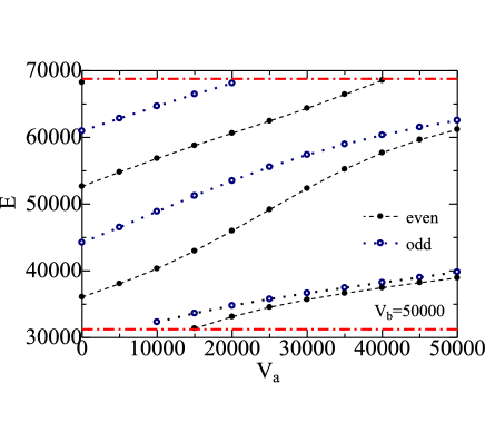
Figure 4: (Color online) The $V_{a}$ dependence of eigenvalues $E_{n}$ for the VDSP ($V_{b}=50000$, $S_{a}=S_{b}=0$, $a=0.01$ and $b=0.02$): bound states appear between lower and upper limits expressed by chain curves. For eigenstates depicted by filled and open circles, $\psi_{+}(x)$ has even- and odd-parity wave functions, respectively, while $\psi_{-}(x)$ has the opposite parity (see text).

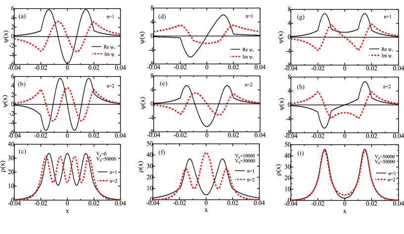
Figure 5: (Color online) Wave function $\psi_{\pm}(x)$ and density probability $\rho(x)$ for the VDSP; $\psi_{\pm}(x)$ for (a) $n=1$ and (b) $n=2$, and (c) $\rho(x)$ for $n=1$ and $n=2$ with $(V_{a},V_{b})=(0,50000)$; $\psi_{\pm}(x)$ for (d) $n=1$ and (e) $n=2$, and (f) $\rho(x)$ for $n=1$ and $n=2$ with $(V_{a},V_{b})=(10000,50000)$; $\psi_{\pm}(x)$ for (g) $n=1$ and (h) $n=2$, and (i) $\rho(x)$ for $n=1$ and $n=2$ with $(V_{a},V_{b})=(50000,50000)$. In (a), (b), (d), (e), (g) and (h), solid and dashed curves express Re $\psi_{+}(x)$ and Im $\psi_{-}(x)$, respectively [Im $\psi_{+}(x)=$ Re $\psi_{-}(x)=0$]. In (c), (f) and (i), solid and dashed curves denote $\rho(x)$ for $n=1$ and $n=2$, respectively ($a=0.01$ and $0.02$).

Figures 5(a) and 5(b) show wave functions for $n=1$ and $n=2$, respectively, with $(V_{a},V_{b})=(0,50000)$. We note that Re $\psi_{+}(x)$ for $n=1$ with $V_{b}=50000$ in Figs. 5(a) have three nodes in contrast with the conventional wisdom that the ground-state wavefunction has a single node. It is the case also for $n=2$ where number of nodes of Re $\psi_{+}(x)$ in Fig. 5(b) is four. This is because wave vectors $k$ for $E_{1}=38948$ and $E_{2}=39831$ with $V_{b}=50000$ have large values. Figure 5(c) shows that density probabilities $\rho(x)$ for $n=1$ and $n=2$ have three and four peaks, respectively.

We introduce $V_{a}=10000$ in the central square potential, for which the wave vector $p$ in the region III is real. Solid (dashed) curves in Figs. 5(d) and 5(e) show Re $\psi_{+}(x)$ (Im $\psi_{-}(x)$) for $n=1$ and $n=2$, respectively. It is noted that the parity of $\psi_{+}(x)$ for $n=2$ is even while that for $n=1$ is odd. This is because $\psi_{+}(x)$ for $n=2$ with $V_{a}=10000$ has the same even parity as that for $n=1$ with $V_{a}=0$, as shown in Fig. 4. Density probabilities $\rho(x)$ for $n=1$ and $n=2$ have two and three peaks, respectively, in Fig. 5(f).

The value of $V_{a}$ is furthermore increased to $V_{a}=50000$, for which $p$ in the region III becomes imaginary. Figures 5(g) and 5(h) show that magnitudes of wave functions for $n=1$ and $n=2$ in the region III are much reduced compared to those in regions II and IV. Then magnitudes of density probabilities in the region III become significantly smaller than those in regions II and IV, as shown in Fig. 5(i).

III.2 Scalar potential only ($V(x)=0$)

Next we study the case of the SDSP, changing $S_{a}$ with fixed $S_{b}=50000$, $V_{a}=V_{b}=0$, $a=0.01$ and $b=0.02$. Figure 6 shows calculated eigenvalues as a function of $S_{a}$, numerical figures of some results being shown also in Table 2. Note that eigenvalues are given for a pair of $\pm E$ [Eq. (105)] although we will hereafter consider the positive eigenvalue only. For eigenvalues shown by filled and open circles, $\psi_{+}(x)$ ($\psi_{-}(x)$) has the even and odd (odd and even) parities, respectively. For $S_{a}=0$, we have six bound states within the allowed range of $18769<E_{n}<68769$ ($n=1-6$) between the lower and upper limits shown by dashed curves. With increasing $V_{a}$, eigenvalues are gradually increased. For $S_{a}\geq 20000$, eigenvalues of $E_{1}$ and $E_{2}$ are quasi-degenerate, but not degenerate Coutinho88 . This trend is the same as that for the VDSP shown in Fig. 4.

$S_{a}$	$n=1$	$n=2$	$n=3$	$n=4$	$n=5$	$n=6$
$\;\;0\;\;$	20708	25901	33130	41443	50290	59317
10000	26381	27912	36321	44871	52510	60547
20000	28963	29238	42876	49214	54937	62666
30000	29994	30042	50417	53138	57791	66274
40000	30539	30548	55317	55730	63393	$-$
50000	30887	30888	57204	57251	$-$	$-$

Table 2 Eigenvalues $E_{n}$ as a function of $S_{a}$ for the SDSP with $S_{b}=50000$, $V_{a}=V_{b}=0$, $a=0.01$ and $b=0.02$, the index $n$ being assigned from the lowest eigenvalue (see Fig. 6).

Calculated wavefunctions and density probabilities are plotted in Figs. 7(a)-7(i). Figures 7(a) and 7(b) show wavefunctions for $n=1$ and $n=2$, respectively, for $(S_{a},S_{b})=(0,50000)$, and Fig. 7(c) denotes relevant density probabilities. With the central barrier potential of $S_{a}=10000$ for which the wave vector $q$ becomes imaginary, magnitudes of the wavefunction and probability density for $n=1$ at $-0.01<x<0.01$ are decreased, as shown in Figs. 7(d)-7(f). Figures 7(g)-7(i) show that for a larger $S_{a}=50000$, magnitudes of $\rho(x)$ and $\psi_{\pm}(x)$ almost completely vanish at $-0.01<x<0.01$.

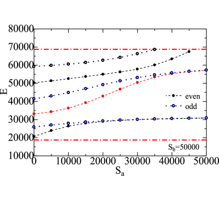
Figure 6: (Color online) The $S_{a}$ dependence of eigenvalues $E_{n}$ for the SDSP ($S_{b}=10000$, $V_{a}=V_{b}=0$, $a=0.01$ and $b=0.02$): bound states appear between lower and upper limits expressed by chain curves. For eigenstates depicted by filled and open circles, $\psi_{+}(x)$ has even- and odd-parity wave functions, respectively, while $\psi_{-}(x)$ has the opposite parity.

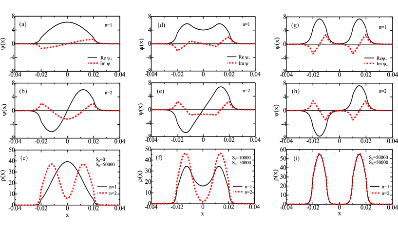
Figure 7: (Color online) Wave function $\psi_{\pm}(x)$ and density probability $\rho(x)$ for SDSP; $\psi_{\pm}(x)$ for (a) $n=1$ and (b) $n=2$, and (c) $\rho(x)$ for $n=1$ and $n=2$ with $(S_{a},S_{b})=(0,50000)$; $\psi_{\pm}(x)$ for (d) $n=1$ and (e) $n=2$, and (f) $\rho(x)$ for $n=1$ and $n=2$ with $(S_{a},S_{b})=(10000,50000)$; $\psi_{\pm}(x)$ for (g) $n=1$ and (h) $n=2$, and (i) $\rho(x)$ for $n=1$ and $n=2$ with $(S_{a},S_{b})=(50000,50000)$. In (a), (b), (d), (e), (g) and (h), solid and dashed curves express Re $\psi_{+}(x)$ and Im $\psi_{-}(x)$, respectively [Im $\psi_{+}(x)=$ Re $\psi_{-}(x)=0$]. In (c), (f) and (i), solid and dashed curves denote $\rho(x)$ for $n=1$ and $n=2$, respectively ($a=0.01$ and $0.02$).

III.3 Equal Scalar and vector potentials ($S(x)=V(x)$)

We study the case of the EDSP [$S(x)=V(x)$], for which the Dirac equation is expressed by one component equation given by

$$\left[\hbar^{2}c^{2}\frac{d^{2}}{dx^{2}}+E^{2}-m^{2}c^{4}-2(mc^{2}+E)V(x)\right]\psi_{+}(x)=0,$$ (120)

$$\psi_{-}(x)=\left(\frac{-i\hbar c}{mc^{2}+E}\right)\frac{d}{dx}\psi_{+}(x).$$ (121)

Figure 8 shows eigenvalues calculated as a function of $S_{a}$ ($=V_{a}$) for fixed $S_{b}=V_{b}=25000$, $a=0.01$ and $b=0.02$, numerical values of some results being shown in Table 3. We notice that the $V_{a}$ dependence of eigenvalues in Fig. 8 is similar to that for the SDSP shown in Fig. 6.

$S_{a}(=V_{a})$	$n=1$	$n=2$	$n=3$	$n=4$	$n=5$	$n=6$	$n=7$
$\;\;0\;\;$	20954	26527	33944	422623	50995	59814	68033
5000	26990	29182	37672	46322	54189	62385	$-$
10000	30255	30882	43879	50724	57152	65381	$-$
15000	31791	31981	50973	54503	60328	$-$	$-$
20000	32665	32731	56190	57167	65430	$-$	$-$
25000	33250	33276	58693	58910	$-$	$-$	$-$

Table 3 Eigenvalues $E_{n}$ as a function of $S_{a}$ ($=V_{a}$) for the EDSP with $S_{b}=V_{b}=25000$, $a=0.01$ and $b=0.02$, the index $n$ being assigned from the lowest eigenvalue (see Fig. 8).

Relevant wavefunctions and density probabilities are shown in Figs. 9(a)-9(i). Although the wavevector $p$ is real for the case of $S_{a}=V_{a}=0$ in Figs. 9(a)-9(c), it becomes imaginary for cases of $S_{a}=V_{a}=5000$ and $25000$ in Figs. 9(d)-9(i). Comparing Figs. 9(a)-9(i) to Figs. 7(a)-7(i), we again notice that wavefunctions and probability densities for the EDSP are quite similar to those for the SDSP.

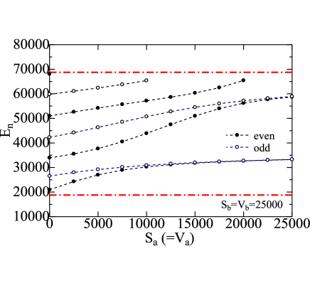
Figure 8: (Color online) The $S_{a}$ ($=V_{a}$) dependence of eigenvalues $E_{n}$ for EDSP ($S_{a}=V_{a}=25000$, $a=0.01$ and $b=0.02$): bound states appear between lower and upper limits expressed by chain curves. For eigenstates depicted by filled and open circles, $\psi_{+}(x)$ has even- and odd-parity wave functions, respectively, while $\psi_{-}(x)$ has the opposite parity.

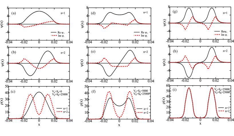
Figure 9: (Color online) Wave function $\psi_{\pm}(x)$ and density probability $\rho(x)$ for the EDSP; $\psi_{\pm}(x)$ for (a) $n=1$ and (b) $n=2$, and (c) $\rho(x)$ for $n=1$ and $n=2$ with $(S_{a},S_{b})=(V_{a},V_{b})=(0,25000)$; $\psi_{\pm}(x)$ for (d) $n=1$ and (e) $n=2$, and (f) $\rho(x)$ for $n=1$ and $n=2$ with $(S_{a},S_{b})=(V_{a},V_{b})=(5000,25000)$ ; $\psi_{\pm}(x)$ for (g) $n=1$ and (h) $n=2$, and (i) $\rho(x)$ for $n=1$ and $n=2$ with $(S_{a},S_{b})=(V_{a},V_{b})=(25000,25000)$. In (a), (b), (d), (e), (g) and (h), solid and dashed curves express Re $\psi_{+}(x)$ and Im $\psi_{-}(x)$, respectively [Im $\psi_{+}(x)=$ Re $\psi_{-}(x)=0$]. In (c), (f) and (i), solid and dashed curves denote $\rho(x)$ for $n=1$ and $n=2$, respectively ($a=0.01$ and $0.02$).

IV Discussion

IV.1 Comparison with results of the Schrödinger equation for the DSP

We may apply the transfer-matrix method adopted in this study to the Schrödinger equation for the DSP. A calculation for the Schrödinger equation goes parallel to that for the Dirac equation, details being provided in the Appendix. The condition of bound states for the DSP is given by Eq. (A53), which is ostensibly the same as Eq. (100) if the relation: $\alpha/k=\beta/q=\gamma/p$ holds. From Eqs. (108)-(110) and (A54), the conceivable range of the bound-state energy $E$ ($>0$) is given by

$${\rm max}(V_{b}-2mc^{2},0) < E_{s}<V_{b}\hskip 14.22636pt\mbox{for $S_{b}=0$ (VDSP)},$$ (122)

$$0 < E_{s}<S_{b}\hskip 14.22636pt\mbox{for $V_{b}=0$ (SDSP)},$$ (123)

$$0 < E_{s}<2S_{b}\hskip 14.22636pt\mbox{for $S_{b}=V_{b}$ (EDSP)},$$ (124)

$$0 < E<V_{b}\hskip 56.9055pt\mbox{in the Schr\"{o}dinger equation},$$ (125)

where $E_{s}=E-mc^{2}$. Bound-state ranges for SDSP and EDSP in the Dirac equation are similar to that in the Schrödinger equation, in contrast to that for the VDSP (Fig. 3).

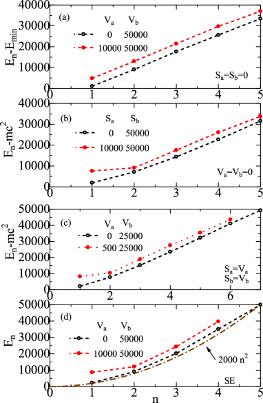
Figure 10: (a) The $n$ dependence of $E_{n}-E_{min}$ for (a) the VDSP of $(V_{a},V_{b})=(0,50000)$ (open circles) and $(10000,50000)$ (filled circles) with $(S_{a},S_{b})=(0,0)$ and $E_{min}=V_{b}-mc^{2}=31231$; (b) $E_{n}-mc^{2}$ for the SDSP of $(S_{a},S_{b})=(0,50000)$ (open circles) and $(10000,50000)$ (filled circles) with $(V_{a},V_{b})=(0,0)$ and $mc^{2}=18769$; (c) $E_{n}-mc^{2}$ with the EDSPs of $(V_{a},V_{b})=(S_{a},S_{b})=(0,25000)$ (open circles) and $(5000,25000)$ (filled circles); (d) $E_{n}$ of the Schrödinger equation (SE) for the DSP with $(V_{a},V_{b})=(0,50000)$ (open circles) and $(10000,50000)$ (filled circles), the chain curve denoting $2000\>n^{2}$. Dashed curves are plotted for guide of eye ($a=0.01$ and $b=0.02$).

We have calculated eigenvalues of the Schrödinger equation for the DSP. Calculated eigenvalues $E_{n}$ are plotted in Fig. 10(d) as a function of $n$ for two sets of $V_{a}$ and $V_{b}$. Eigenvalues for $(V_{a},V_{b})=(0,50000)$ and $(10000,50000)$ approximately follow $E_{n}\simeq 2000\>n^{2}$ which is shown by the chain curve. Note that the $E_{n}\propto n^{2}$ law is exactly realized in the limit of $V_{b}=\infty$ [Eq. (A58)].

The $n$ dependence of $E-E_{min}$ for the VDSP studied in Secs. III A is shown in Fig. 10(a) where $E_{min}={\rm max}(V_{b}-mc^{2},mc^{2})=31231$. Figures 10(b) and 10(c)) show the $n$-dependence of eigenvalues of $E-mc^{2}$ for the SDSP and EDSP, respectively, which are studied in Secs. III B and III C. We expect from Figs. 10(a)-10(c) that that the eigenvalue in the Dirac equation for scalar and vector DSPs approximately follows a linear $n$ dependence for adopted parameters of $V_{a}\ll V_{b}$ and $S_{a}\ll S_{b}$.

We have calculated the wavefunction and probability density in the Schrödinger equation for the DSP with $(V_{a},V_{b})=(0,50000)$, $(10000,50000)$ and $(50000,50000)$ whose results are plotted in Figs. 11(a)-11(f). We note that wavefunctions and probability densities for $(V_{a},V_{b})=(0,50000)$ in Figs. 11(a) and 11(b) are similar to $\psi_{+}(x)$ and $\rho(x)$ of the Dirac equation for the SDSP shown in Figs. 7(a)-7(c) and to those for the EDSP shown in Figs. 9(a)-9(c), although they are quite different from those for the VDSP shown in Figs. 5(a)-5(c). It is the case also for $(V_{a},V_{b})=(10000,50000)$ in Figs. 11(c) and 11(d) and for $(V_{a},V_{b})=(50000,50000)$ in Figs. 11(e) and 11(f).

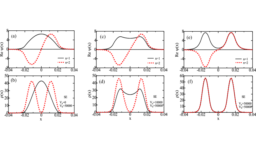
Figure 11: (Color online) Wave function $\psi(x)$ and density probability $\rho(x)$ of the Schrödinger equation (SE) for the DSP; (a) Re $\psi(x)$ and (b) $\rho(x)$ for $(V_{a},V_{b})=(0,50000)$; (c) Re $\psi(x)$ and (d) $\rho(x)$ for $(V_{a},V_{b})=(100000,50000)$; (e) Re $\psi(x)$ and (f) $\rho(x)$ for $(V_{a},V_{b})=(500000,50000)$. Solid and dashed curves express results for $n=1$ and $n=2$, respectively.

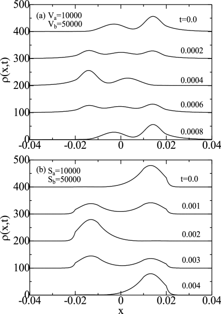
Figure 12: Time dependence of $\rho(x,t)$ for (a) the VDSP of $(V_{a},V_{b})=(10000,50000)$, and (b) the SDSP of $(S_{a},S_{b})=(10000,50000)$, results being successively shifted for clarity of figures ($a=0.01$ and $b=0.02$).

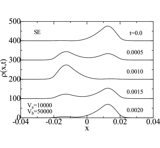
Figure 13: Time dependence of $\rho(x,t)$ of the Schrödinger equation (SE) for $(V_{a},V_{b})=(10000,50000)$, results being successively shifted for clarity of figure ($a=0.01$ and $b=0.02$).

IV.2 Tunneling through the central barrier

We may study the tunneling of a particle through the central potential barrier. As an initial Gaussian-like wave packet, we assume a pair of the states for $n=1$ and $n=2$ as given by

$$\Psi(x,t) = \left({\begin{array}[]{*{20}c}\psi_{+}(x,t)\\ \psi_{-}(x,t)\\ \end{array}}\right)=\frac{1}{\sqrt{2}}\left({\begin{array}[]{*{20}c}\psi_{1+}(x)\\ \psi_{1-}(x)\\ \end{array}}\right)\>e^{-iE_{1}t/\hbar}+\frac{1}{\sqrt{2}}\left({\begin{array}[]{*{20}c}\psi_{2+}(x)\\ \psi_{2-}(x)\\ \end{array}}\right)\>e^{-iE_{2}t/\hbar},$$ (132)

where $\psi_{n\pm}(x)$ denotes spinor of the stationary wave function and $E_{n}$ signifies an eigenvalue of state $n$ ($=1,2$). The time-dependent probability density $\rho(x,t)$ is given by

$$\rho(x,t) = |\psi_{+}(x,t)|^{2}+|\psi_{-}(x.t)|^{2}.$$ (133)

It is straightforward to calculate $\rho(x,t)$ because we have obtained $\psi_{n\pm}(x)$ and $E_{n}$ for $n=1,2$ in the preceding Sec. III.

Figure 12(a) shows $\rho(x,t)$ for the VDSP with $(V_{a},V_{b})=(10000,50000)$. At $t=0.0$, $\rho(x,0)$ consists of two Gaussian-like wave packets because stationary wave functions of $\psi_{1\pm}(x)$ and $\psi_{2\pm}(x)$ have multiple nodes in Figs. 5(d) and 5(e). The period of the oscillation is $T=2\pi/\Delta E_{12}=0.000786$ for $\Delta E_{12}=E_{2}-E_{1}=7998$. The time dependence of $\rho(x,t)$ for the SDSP with $(S_{a},S_{b})=(10000,50000)$ shown in Fig. 12(b) has the period of $T=0.0041$ for $\Delta E_{12}=1531$. The time dependence of $\rho(x,t)$ for the EDSP is similar to that for the SDSP (relevant result not shown).

Figure 13 shows $\rho(x,t)$ of the Schrödinger equation for the DSP with $(V_{a},V_{b})=(10000,50000)$ which yields $T=0.00184$. We note that $\rho(x,t)$ of the Schrödinger equation is similar to that for the SDSP in Fig. 12(b) but not to that for the VDSP in Fig. 12(a).

V Conclusion

Exact expressions of bound states for scalar and vector DSPs in the one-dimensional Dirac equation have been obtained with the use of the elegant transfer-matrix method. Our calculations have shown that although results of the Dirac equation for scalar and vector DSPs reduce to those of the Schrödinger in the nonrelativistic limit, they have the difference and similarity in general as follows:

(i) The bound-state energy range of the Dirac equation for the VDSP is different from those for the SDSP and EDSP (Fig. 3),

(ii) The bound-state energy $E_{n}$ has an approximate linear $n$ dependence in the Dirac equation for adopted scalar and vector DSPs with small central potential barriers, while it is approximately given by $E_{n}\propto n^{2}$ in the Schrödinger equation (Fig. 10), and

(iii) The wave function and probability density of the Dirac equation for the VDSP are rather different from those of the Dirac equation for the SDSP and EDSP, and also from those of Schrödinger equation (Figs. 5, 7, 9 and 11).

As for the item (i), Eq. (122) implies that the bound-state energy range for the vector potential depends on the order of taking two limits of $mc^{2}\rightarrow\infty$ and $V_{b}\rightarrow\infty$. If we first take the nonrelativistic limit of $mc^{2}\rightarrow\infty$, the bound-state range becomes $0<E_{s}<V_{b}\rightarrow\infty$ ($E_{s}=E-mc^{2}$) for infinite confining potential, in agreement with that of the Schrödinger equation in Eq. (125): $0<E<V_{b}\rightarrow\infty$, as shown in Eq. (119). However, if we first take the limit of $V_{b}\gg mc^{2}$, the range for the bound state becomes $V_{b}-2mc^{2}<E_{s}<V_{b}$, which disagrees with the relevant result of the Schrödinger equation. On the other hand, for the scalar potential, Eq. (123) always yields $0<E_{s}<S_{b}$ for the positive eigenvalue in agreement with Eq. (125) of the Schrödinger equation. This is consistent with Ref. Alberto96 in which Alberto, Fiolhals and Gil pointed out that a calculation with the scalar potential avoids a difficulty realized with the vector potential, in studying a single square-well system with an infinite confining potential [Eq. (115)].

Considering the fact that the double-well potential has been extensively studied within the nonrelativistic treatment Thorwart01 , we expect that scalar and vector DSPs in the Dirac equation play important roles in studying relativistic double-well systems, to which our method may be applied with various generalizations. Quite recently our nonrelativistic calculations have shown that an asymmetry in the double-well potential yields interesting quantum phenomena Hasegawa12 ; Hasegawa13 . An application of the Dirac equation to an asymmetric DSP is under consideration and results will be reported in a separate paper.

*

Appendix A Schrödinger equation for the DSP

We obtain the bound-state solution of the Schrödinger equation

$$\left[-\frac{\hbar^{2}}{2m}\>\frac{d^{2}}{dx^{2}}+V(x)\right]\psi(x) = E\psi(x),$$ (A1)

for the DSP given by Eq. (12). Wave functions in five regions I$-$V are given by

$$\psi_{I}(x) = A_{1}\>e^{iqx}+B_{1}\>e^{-iqx}\hskip 28.45274pt\mbox{for $x\leq-b$},$$ (A2)

$$\psi_{II}(x) = A_{2}\>e^{ikx}+B_{2}\>e^{-ikx}\hskip 28.45274pt\mbox{for $-b<x\leq-a$},$$ (A3)

$$\psi_{III}(x) = A_{3}\>e^{ipx}+B_{3}\>e^{-ipx}\hskip 28.45274pt\mbox{for $-a<x\leq a$},$$ (A4)

$$\psi_{IV}(x) = A_{4}\>e^{ikx}+B_{4}\>e^{-ikx}\hskip 28.45274pt\mbox{for $a<x\leq b$},$$ (A5)

$$\psi_{V}(x) = A_{5}\>e^{iqx}+B_{5}\>e^{-iqx}\hskip 28.45274pt\mbox{for $x>b$},$$ (A6)

with

$$k = \frac{\sqrt{2mE}}{\hbar},$$ (A7)

$$p = \frac{\sqrt{2m(E-V_{a})}}{\hbar},$$ (A8)

$$q = \frac{\sqrt{2m(E-V_{b})}}{\hbar},$$ (A9)

where $A_{i}$ ($B_{i}$) ($i=1-3$) denote magnitudes of wave functions traveling rightwards (leftwards), and $m$ is mass of a particle. From the matching conditions for wave functions and their derivatives at the boundaries at $x=\pm a$ and $x=\pm b$, we obtain

$$\left({\begin{array}[]{*{20}c}{e^{-iqb}}&{e^{iqb}}\\ {q\>e^{-iqb}}&{-q\>e^{iqb}}\\ \end{array}}\right)\left({\begin{array}[]{*{20}c}{A_{1}}\\ {B_{1}}\\ \end{array}}\right) = \left({\begin{array}[]{*{20}c}{e^{-ikb}}&{e^{ikb}}\\ {k\>e^{-ikb}}&{-k\>e^{ikb}}\\ \end{array}}\right)\left({\begin{array}[]{*{20}c}{A_{2}}\\ {B_{2}}\\ \end{array}}\right),$$ (A18)

$$\left({\begin{array}[]{*{20}c}{e^{-ika}}&{e^{ika}}\\ {k\>e^{-ika}}&{-k\>e^{ika}}\\ \end{array}}\right)\left({\begin{array}[]{*{20}c}{A_{2}}\\ {B_{2}}\\ \end{array}}\right) = \left({\begin{array}[]{*{20}c}{e^{-ipa}}&{e^{ipa}}\\ {p\>e^{-ipa}}&{-p\>e^{ipa}}\\ \end{array}}\right)\left({\begin{array}[]{*{20}c}{A_{3}}\\ {B_{3}}\\ \end{array}}\right),$$ (A27)

$$\left({\begin{array}[]{*{20}c}{e^{ipa}}&{e^{-ipa}}\\ {p\>e^{ipa}}&{-p\>e^{-ipa}}\\ \end{array}}\right)\left({\begin{array}[]{*{20}c}{A_{3}}\\ {B_{3}}\\ \end{array}}\right) = \left({\begin{array}[]{*{20}c}{e^{ika}}&{e^{-ika}}\\ {k\>e^{ika}}&{-k\>e^{-ika}}\\ \end{array}}\right)\left({\begin{array}[]{*{20}c}{A_{4}}\\ {B_{4}}\\ \end{array}}\right),$$ (A36)

$$\left({\begin{array}[]{*{20}c}{e^{ikb}}&{e^{-ikb}}\\ {k\>e^{ikb}}&{-k\>e^{-ikb}}\\ \end{array}}\right)\left({\begin{array}[]{*{20}c}{A_{4}}\\ {B_{4}}\\ \end{array}}\right) = \left({\begin{array}[]{*{20}c}{e^{iqb}}&{e^{-iqb}}\\ {q\>e^{iqb}}&{-q\>e^{-iqb}}\\ \end{array}}\right)\left({\begin{array}[]{*{20}c}{A_{5}}\\ {B_{5}}\\ \end{array}}\right).$$ (A45)

Transfer matrix is given by

$$\left({\begin{array}[]{*{20}c}{A_{1}}\\ {B_{1}}\\ \end{array}}\right) = \left({\begin{array}[]{*{20}c}{T_{11}}&{T_{12}}\\ {T_{21}}&{T_{22}}\\ \end{array}}\right)\left({\begin{array}[]{*{20}c}{A_{5}}\\ {B_{5}}\\ \end{array}}\right).$$ (A52)

We note that Eqs. (A18)-(A45) are equivalent to Eqs. (58)-(85) for the Dirac equation when we read $\alpha=k$, $\beta=q$ and $\gamma=p$. The condition for the bound state is given by

$$T_{11} = \frac{e^{2iqb}}{16k^{2}qp}\{(k+p)^{2}\left[(k+q)^{2}\>e^{2i[k(a-b)-pa]}-(k-q)^{2}\>e^{-2i[k(a-b)-pa]}\right]$$ (A53)

$$+ (k-p)^{2}\left[(k-q)^{2}\>e^{-2i[k(a-b)+pa]}-(k+q)^{2}\>\>e^{2i[k(a-b)+pa]}\right]$$

$$+ 2(k^{2}-q^{2})(k^{2}-p^{2})\left[\>e^{2ipa}-e^{-2ipa}\right]\}=0.$$

Bound states appear at

$$0<E<V_{b},$$ (A54)

for which $k$ is real and $q$ is purely imaginary: plane waves in regions II and IV and evanescent waves in regions I and V.

It is necessary to numerically solve the transcendental equation (A53) for given parameters of $m$, $V_{a}$, $V_{b}$, $a$, $b$. Once an eigenvalue is obtained from Eq. (A53), matrix calculations determine coefficients of $A_{i}$, $B_{i}$ ($i=2$ to 4) and $B_{1}$ with $A_{1}=B_{5}=0$ for an assumed value of $A_{5}=C$ and $B_{5}=0$, as was made for the Dirac equation. The magnitude of $C$ is fixed by the normalization condition:

$$\int_{-\infty}^{\infty}|\psi(x)|^{2}\>dx=1.$$ (A55)

In the limit of $V_{a}=0$ or in the limit of $a=0$, Eq. (A53) becomes

$$\frac{1}{4kq}\left[(q+k)^{2}e^{-2ikb}-(q-k)^{2}e^{2ikb}\right] = 0,$$ (A56)

which leads to the result for the single square-well potential

$$\frac{2k\kappa}{k^{2}-\kappa^{2}} = \tan(2kb)\hskip 28.45274pt\left(\kappa=\frac{\sqrt{2m(V_{b}-E)}}{\hbar}\right).$$ (A57)

In the limit of $V_{b}\rightarrow\infty$, Eq. (A57) yields the well-known result

$$E_{n} = \frac{n^{2}\pi^{2}\hbar^{2}}{8mb^{2}}\hskip 28.45274pt\mbox{($n=1,2,\cdots$)}.$$ (A58)

References

- (1) W. Greiner, Relativistic Quantum MechanicsWave Equations (Springer-Verlag, Berlin, 1990).
- (2) M. J. Thomspn and B. H. McKellr, Am. J. Phys. 59, 340(1991).
- (3) H. Nitta, T. Kudo and H. Minowa, Am. J. Phys. 67, 966 (1999).
- (4) S. De Leo and P. P. Rotelli, arXiv:hep-th/0607176.
- (5) P. Krekora, Q. Su, and R. Grobe, Phys. Rev. Lett. 92, 040406 (2004).
- (6) S. D. Bosanac, J. Phys. A: Math. Theor. 40, 8991 (2007).
- (7) B. L. Coulter and C. G. Adler, Am. J. Phys. 39 (1971) 305.
- (8) G. Gumbs and D. Kiang, Am. J. Phys. 54 (1986) 462.
- (9) A. B. Coutinho, Y. Nogami, and F. M. Toyama, Am. J. Phys. 56 (1988) 904.
- (10) P. Alberto, C. Fiolhals, and V. M. S. Gil, Eur. J. Phys. 17 (1996) 19.
- (11) A. D. Alhaidari and E. El Aaoud, Proc. Filth Saudi Physical Siciety 1370 (2011) 21.
- (12) X. U. Ying, L. U. Meng, and S. U. Ru-Keng, Commun. Theor. Phys. (Beijing, China) 41 (2004), 859.
- (13) Although Ref. Ying04 discussed an application of the Dirac equation to the double square-well potential, its eigenvalue condition is not correct and disagrees with our result [Eq. (100)]. Actually Eqs. (73) and (78) in Ref. Ying04 do not reduce to the relevant condition for the single square-well potential in the limit of , , or (in our notations).
- (14) M. Thorwart, M. Grifoni, and P. Hänggi, Annals Phys. 293, 14 (2001).
- (15) E. Peacock-López, Chem. Educator 11, 383 (2006).
- (16) A. Acus and A. Dargys, Phys. Scr. 84, 015703 (2011).
- (17) S. T. Tserkis, Ch. C. Moustakidis, S. E. Massen, and C. P. Panos, arXiv: 1307.1104.
- (18) H. Hasegawa, Phys. Rev. 86, 061104 (2012).
- (19) H. Hasegawa, Physica A 392 6232 (2013).