Response to Selection for continuous traits: an alternative to the breeder’s and Lande’s equations.

Abstract

The breeder’s equation is a cornerstone of quantitative genetics and is widely used in evolutionary modeling. The equation, which reads $R=h^{2}S$, relates response to selection $R$ (the mean phenotype of the progeny) to the selection differential $S$ (mean phenotype of selected parents) through a simple proportionality relation. The validity of this relation however relies strongly on the normal (Gaussian) distribution of the parent genotype, which is an unobservable quantity and cannot be ascertained. In contrast, we show here that if the fitness (or selection) function is Gaussian, an alternative, exact linear equation of the form $R^{\prime}=j^{2}S^{\prime}$ can be derived, regardless of the parental genotype distribution. Here $R^{\prime}$ and $S^{\prime}$ stand for the mean phenotypic lag with respect to the mean of the fitness function in the offspring and selected populations. To demonstrate this relation, we derive the exact functional relation between the mean phenotype in the selected and the offspring population and deduce all cases that lead to a linear relation between the mean phenotypes of progeny and selected parents. These results, which are confirmed by individual based numerical simulations, generalize naturally to the concept of $G$ matrix and the multivariate Lande’s equation $\Delta\mathbf{\bar{z}}=GP^{-1}\mathbf{S}$. The linearity coefficients of the alternative equation are not changed by selection. The alternative equation can thus be more suitable for long term evolutionary studies than the $G$ matrix.

I Introduction.

The breeder’s equation for the evolution of quantitative traits for additive genetic effects, introduced by Lush Lush (1943) is widely used both in artificial and natural selection theory and experiments Falconer and Mackay (1995); Lynch and Walsh (1998); Lande (1976); Heywood (2005) and appears in all textbooks of quantitative genetic. The scalar equation $R=h^{2}S$, or its vectorial version $\Delta\bar{\mathbf{z}}=GP^{-1}\mathbf{S}$ ascertain that the response to selection (mean phenotype of offspring) and the selection differential (mean phenotype of selected parents) are related through a linear relation which is the ratio of genotype to phenotype variances, $h^{2}$.

Use of the breeder’s equation and its underlying assumptions have been criticized by many authors Heywood (2005); Gienapp and al. (2008); Pigliucci (2006); Kruuk (2004); Pemberton (2010). One fundamental assumption of the breeder’s equation is the normal (Gaussian) distribution of the breeding value (genotype) and environment factors. Authors who demonstrate the linear relation Falconer and Mackay (1995); Lynch and Walsh (1998); Kimura and Crow (1978); Crow and Kimura (2009); Lande (1979); Lande and Arnold (1983); Nagylaki (1992) assume normal distribution for the above quantities or the analogous hypothesis of linearity of the parent-offspring regression (see Appendix/Parent-offspring regression). When this assumption is relaxed, the breeder’s equation is no longer valid and one has to resort to a system of hierarchical moment (or alternatively, cumulant) equations to describe the changes ; in general, this system is not closed and the moments of a given order depend on moments of higher order Turelli and Barton (1990).

The assumption of a Gaussian distribution of the genotype can be criticized on several grounds Pigliucci (2006); Pigliucci and Schlichting (1997); Geyer and Shaw (2008). For example, the very act of selection causes the genotype distribution to deviate from a Gaussian Turelli and Barton (1990, 1994) (see also equation 6 below). Another important case is when the genotype is a cross between different breeds due to external gene flow or the breeder’s scheme. In many cases, the phenotype can have a bell shape and thus is assumed to be Gaussian, when the genotype is indeed far from it (see for example figure 2a). It is sometimes argued that even if the breeding value does not follow a normal distribution, a scale can be used to restore it to a normal distribution. Such a scale however will also distort the distribution of environment factors and the assumptions of breeder’s equation are violated even in this case.

For additive genetic effects and in the absence of epistasis and dominance, I derive here a precise functional relation between the mean of the trait in the selected subpopulation and in their progeny for the general case. The mathematical formulation is close to the framework used by many authors such as Slatkin, Lande and Karlin Slatkin (1970); Lande (1979); Karlin (1979). I then use a standard tool of functional analysis, the Fourier transform, to deduce all the cases taht lead to a linear relation between the response $R$ and the selection differential $S$, regardless of the selection function. These cases imply a precise form of the distributions of genotype and environment factors, and I show that the proportionality factor between $R$ and $S$ is the heritability coefficient $h^{2}$ only if these distributions are normal.

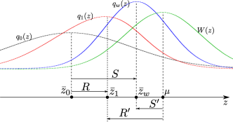
Figure 1: Schematic representation of the selection lag $S^{\prime}$, the response lag $R^{\prime}$ and their relation to the selection differential $S$ and the response $R$. The mean phenotype of parental generation $\bar{z}_{0}$, selected population $\bar{z}_{w}$, the progeny $\bar{z}_{1}$ and the peak of selection function$\mu$ are represented on the phenotype axis $z$. Dashed curves represent a sketch of the distributions of parental phenotype $q_{0}(z)$, selected parents $q_{w}(z)$, the progeny $q_{1}(z)$ and the selection function $W(z)$.

The genotype however is not observable or controllable and its normal distribution cannot be assumed a priori. I show that if instead of the genotype, the fitness function and environment factors are Gaussian, then a new linear relation can be obtained in the form of

$$R^{\prime}=j^{2}S^{\prime}$$ (1)

regardless of the genotype distribution. Here $R^{\prime}$ and $S^{\prime}$ are the mean phenotypic lag with respect to the mean of the fitness function of the progeny and the selected population (Figure 1). The $j^{2}$ coefficient contains only the width of the fitness function and environment factors. The use of a Gaussian selection function, both in artificial and natural selection (as an approximation of stabilizing selection) is widespread Lande (1976); Kimura and Crow (1978); Lewontin (1964); Zhang and Hill (2010) and the above relation is potentially as useful as the standard breeder’s equation.

The advantage is more critical when the breeder’s or Lande’s equations are used in long term evolution, where the variance of the genotype (or the $G$ matrix) also varies and $h^{2}$ cannot be assumed to remain constant Pigliucci and Schlichting (1997); Gavrilets and Hastings (1995); Roff (2000) ; in contrast, the relation (1) remains valid if each round of selection uses a Gaussian fitness function.

The above results generalize naturally to multivariate trait selection where the alternative Lande’s equation is

$$\mathbf{R}^{\prime}=(\Omega+E)\Omega^{-1}\mathbf{S}^{\prime}$$ (2)

where $\mathbf{R}^{\prime}$ and $\mathbf{S}^{\prime}$ are the vectorial phenotype lag, and $\Omega$ and $E$ are the covariance matrices of the fitness function and the environment respectively.

The Fisher’s fundamental theorem states that “the rate of increase in fitness of any organism at any time is equal to its genetic variance in fitness at that time”. The alternative equations (1) or (2) could thus seem unusual, as the linearity coefficient or matrix does not contain the genetic variance. There is however no contradiction : both quantities $R^{\prime}$ and $S^{\prime}$ depend on the genetic variance but their ratio is not. All the above results are confirmed by individual based numerical simulations.

This article is organized as follows : in the Results section, I first derive the general functional relationship between $R$ and $S$; the second subsection is devoted to all the cases where these two quantities can be linearly related, including the special case of the breeder’s equation. The alternative breeder’s equation is derived in the third subsection and all the results are generalized to selection on multiple traits in the fourth subsection. The above results are put into perspective in the Discussion section. Technical details such as the use of Fourier transforms and numerical simulations are treated in the Appendix.

II Results.

General results.

Consider a continuous phenotype $Z$, which is the result of additive genetic effect $Y$ and the environment $\xi$ Visscher and al. (2008)

$$Z=Y+\xi$$

The term environment encompasses here any source of noise that causes the observed phenotype $z$ to deviate from the (unobserved) breeding value $y$ Wright (1920); Lynch and Walsh (1998); Raj and van Oudenaarden (2008). In the following, the population distribution of the breeding value (genotype) and its variance in the parental generation are denoted $p_{0}(y)$ and $\sigma_{A}^{2}$. The environment effect is captured by the distribution law $f(z|y)$, the probability density of observing phenotype $z$ with the given genotype $y$. We will suppose that $f$ is a symmetric function of its argument of the form $f(z|y)=f(z-y)$.

A subpopulation among the parental generation is selected according to a fitness or selection function $W(z)$, the proportion of phenotypes in $[z,z+dz[$ to be selected for the production of the next generation. The selected individuals produce offspring which will constitute the next generation. As we will show below, the response $R$ (the mean of the phenotype trait in the offspring) and the selection differential $S$ (the mean of the phenotype trait in the selected parents) are given by

$$R=E(Z_{1}) = \frac{1}{\bar{W}}\iint_{\mathbb{R}^{2}}yp_{0}(y)W(z)f(z-y)dydz$$ (3)

$$S=E(Z_{w}) = \frac{1}{\bar{W}}\iint_{\mathbb{R}^{2}}zp_{0}(y)W(z)f(z-y)dydz$$ (4)

where $\bar{W}$ is the mean fitness of parental generation. The above equations (3,4) are used for example by Lande Lande (1979), although their derivation there depended on the normal distribution of the genotype. I derive these equations here for the more general case.

Before going into the details of calculations, note that the genotype distribution $p_{0}(y)$ and the selection function $W(z)$ play a symmetric role in the above expressions. In the following sections, we will explore specific functional forms of $p_{0}(y)$ and $W(z)$ which lead to a linear relationship between $R$ and $S$. Because of the symmetric role of these two functions however, once a particular relation is obtained for a specific form of $p_{0}(y)$ regardless of $W(z)$, an analogous relationship can be obtained for a similar form of $W(z)$ regardless of $p_{0}(y)$. This is what leads us to an alternative form of the breeder’s equation.

Let us now derive the equations (3,4). We note that the distribution of the phenotype $Z$ in the parental generation is given by

$$q_{0}(z)=\int_{\mathbb{R}}p_{0}(y)f(z|y)dy$$ (5)

We will denote its variance by $\sigma_{P}^{2}$.

The distribution of the phenotype $z$ in the parental population selected according to the fitness function $W(z)$ is

$$q_{w}(z)=\frac{1}{\bar{W}}q_{0}(z)W(z)$$

where $\bar{W}$ is the mean fitness of the parental generation

$$\bar{W} = \int_{\mathbb{R}}q_{0}(z)W(z)dz$$

$$= \iint_{\mathbb{R}^{2}}p_{0}(y)W(z)f(z|y)dydz$$

The genotype distribution of the selected population is Turelli and Barton (1994)

$$p_{w}(y) = \frac{1}{\bar{W}^{\dagger}}\int_{\mathbb{R}}p_{0}(y)f(z|y)W(z)dz$$ (6)

$$= \frac{1}{\bar{W}^{\dagger}}p_{0}(y)W^{\dagger}(y)$$ (7)

where

$$W^{\dagger}(y)=\int_{\mathbb{R}}W(z)f(z|y)dz$$ (8)

is the genotype fitness function, i.e. the convolution of the phenotype fitness function by the environment factors. $\bar{W}^{\dagger}$ is the mean genotype fitness :

$$\bar{W}^{\dagger} = \int_{\mathbb{R}}p_{0}(y)W^{\dagger}(y)dy$$

$$= \iint_{\mathbb{R}^{2}}p_{0}(y)W(z)f(z|y)dydz$$

Note that $\bar{W}=\bar{W}^{\dagger}$ as both these quantities are defined by the same double integration over the domains of $y$ and $z$.

For a large, randomly mating population, reproduction gives for the distribution of breeding values in the next generation Slatkin (1970); Karlin (1979); Bulmer (1985); Turelli and Barton (1994)

$$p_{1}(y)=\iint_{\mathbb{R}^{2}}p_{w}(y_{a})p_{w}(y_{b})L\left(y-(y_{a}+y_{b})/2\right)dy_{a}dy_{b}$$

The exact form of the probability density $L(y)$ that captures the inheritance process (recombination, segregation, …) is not important here ; Turelli and Barton (Turelli and Barton (1994)) for example use a normal distribution for $L(y)$ in the framework of the infinitesimal model. For our purpose, it is enough to suppose that the mean of the distribution $L(y)$ is zero, i.e. $\int_{y}yL(y)dy=0$ which is valid in the absence of dominance and epistasis effects Turelli and Barton (1990) (see also Appendix/Segregation density function).

The phenotype distribution of the progeny is

$$q_{1}(z)=\int_{\mathbb{R}}p_{1}(y)f(z|y)dy$$ (9)

We now make the further assumption that (i) the environment and genotype are independent random variables, so that $f(z|y)=f(z-y)$ and therefore the variances are additive : $\sigma_{P}^{2}=\sigma_{A}^{2}+\sigma_{E}^{2}$ and (ii) environment effects are of zero mean ($\int_{x}xf(x)dx=0$) and symmetric ($f(-x)=f(x)$ ). An environmental noise with such a distribution law does not change the mean of the random variable : $E(Z)=E(Y+\xi)=E(Y)$. Therefore, the mean phenotype of the offspring is

$$R=E(Z_{1}) = E(Y_{1})$$ (10)

$$= \int_{\mathbb{R}}yp_{1}(y)dy$$

$$= (1/2)\iint_{\mathbb{R}^{2}}(y_{a}+y_{b})p_{w}(y_{a})p_{w}(y_{b})dy_{a}dy_{b}$$

$$= \int_{\mathbb{R}}yp_{w}(y)dy$$

$$= \frac{1}{\bar{W}}\iint_{\mathbb{R}^{2}}yp_{0}(y)W(z)f(z-y)dydz$$ (11)

which is the equation (3). Note that the first lines of the above equations merely state that the expectations of the breeding’s value of parent and offspring are equal for purely additive traits.

On the other hand, the mean phenotype of the selected parents is

$$S=E(Z_{w}) = \int_{\mathbb{R}}zq_{w}(z)dz$$

$$= \frac{1}{\bar{W}}\int_{\mathbb{R}}zq_{0}(z)W(z)dz$$

$$= \frac{1}{\bar{W}}\iint_{\mathbb{R}^{2}}zp_{0}(y)W(z)f(z-y)dydz$$

which is the equation (4).

Note that for an asexually reproducing organism, or for a sexually reproducing population which remains at Hardy-Weinberg equilibrium after selection-reproduction, we would have $p_{1}(y)=p_{w}(y)$ ; this would again lead to the same equation (10) and the same response (3). The conditions for the existence of multilocus Hardy-Weinberg equilibrium were analyzed by Karlin and Liberman Karlin and Liberman (1979a, b) who concluded that for additive traits, the equilibrium is stable for a wide range of recombination distributions.

Conditions for proportionality of $R$ and $S$.

The relations (3,4) show that the selection differential $S$ and the response $R$ to it are related through a functional equation involving three factors : genotype distribution, the selection function and the environmental noise. It is far from obvious that $R$ and $S$ could be proportional.

Fourier transforms (FT) in functional analysis play a role analogous to logarithms in algebra, and part of their usefulness is due to the fact that they transform convolution products into simple products. They are useful for clarifying the $R-S$ relation, where we can transform the double integrations into simple ones. Here $\tilde{u}(k)$ designates the FT of the function $u(x)$ and $a*$ is the complex conjugate of $a$ (see Appendix/Fourier Transforms). We set the origin of the breeding values at its mean in the parental population, i.e. $\int_{\mathbb{R}}yp_{0}(y)dy=0$. The response and selection differential are

$$R=\frac{i}{2\pi\bar{W}}\int_{\mathbb{R}}\tilde{W}^{*}(k)\tilde{p}_{0}^{\prime}(k)\tilde{f}(k)dk$$

and

$$S = \frac{i}{2\pi\bar{W}}\int_{\mathbb{R}}\tilde{W}^{*}(k)\left[\tilde{p}_{0}^{\prime}(k)\tilde{f}(k)+\tilde{p}_{0}(k)\tilde{f}^{\prime}(k)\right]dk$$ (12)

$$= R+\frac{i}{2\pi\bar{W}}\int_{\mathbb{R}}\tilde{W}^{*}(k)\tilde{p}_{0}(k)\tilde{f}^{\prime}(k)dk$$

We see that $S$ and $R$ can be proportional if the second term of the r.h.s. of equation (12) is proportional to $R$ ; this will be true, regardless of the selection function $W$, if

$$\tilde{p}_{0}(k)\tilde{f}^{\prime}(k)=a\tilde{p}_{0}^{\prime}(k)\tilde{f}(k)$$ (13)

where $a$ is an arbitrary constant. Equation (13) is the necessary and sufficient condition that defines the functional shape of the genotype distribution and the environment noise compatible with the proportionality of $R$ and $S$ regardless of the selection function. If condition (13) is fulfilled, then

$$R=(1+a)^{-1}S$$

On the other hand, eq. (13) can be seen as a differential equation whose solution is given by

$$\tilde{f}(k)=b\tilde{p}_{0}(k)^{a}$$ (14)

where $b$ is another arbitrary constant.

If $\tilde{f}(k)$ and $\tilde{p}_{0}(k)$ are both Gaussians, i.e.,

$$\tilde{f}(k) = \text{$\exp$}\left(-\sigma_{E}^{2}k^{2}/2\right)$$

$$\tilde{p}_{0}(k) = \exp\left(-\sigma_{A}^{2}k^{2}/2\right)$$

then the relation(14) is satisfied by

$$a=\sigma_{E}^{2}/\sigma_{A}^{2}$$

and we retrieve the usual breeder’s equation $R=h^{2}S$ where $h^{2}=\sigma_{A}^{2}/(\sigma_{A}^{2}+\sigma_{E}^{2})$. Of course, if $\tilde{f}(k)$ and $\tilde{p}_{0}(k)$ are of the above form, their inverse Fourier transforms represent normal distributions of width $\sigma_{E}$ and $\sigma_{A}$ respectively (see Appendix/Fourier Transforms).

We see however that even if the strict condition (14) is fulfilled, the proportionality constant need not be $h^{2}$. Consider for example the class of stretched exponential functions $\phi(k)=\exp(-|k|^{\alpha})$ which generalizes Gaussians (case $\alpha=2$). Set $\tilde{f}(k)=\phi(\sigma_{E}k)$, $\tilde{p}_{0}(k)=\phi(\sigma_{A}k)$. The inverse Fourier transform of these functions gives the distribution of the genotype $Y$ and environment effect $E$ and it is straightforward to show that as for the Gaussian case, $\mbox{Var}(E)/\mbox{Var}(Y)=\sigma_{E}^{2}/\sigma_{A}^{2}$. Condition (14) however is satisfied this time with $a=\sigma_{E}^{\alpha}/\sigma_{A}^{\alpha}$ and therefore the realized heritability $h^{\alpha}=R/S$ is

$$h^{\alpha}=\frac{\sigma_{A}^{\alpha}}{\sigma_{A}^{\alpha}+\sigma_{E}^{\alpha}}$$

The above examples were to emphasize the fact that selection-independent proportionality is achieved only for particular pairs of genotype/environment distributions. In general, as shown in figure 2, the realized heritability is not constant and depends critically on the selection function $W(z)$.

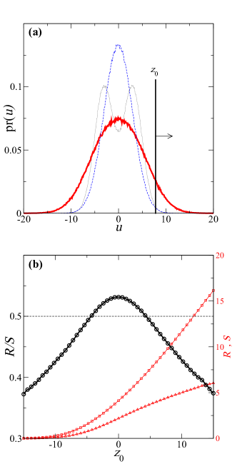
Figure 2: Individual based numerical simulation of the selection process and its comparison to theoretical results. (a) $10^{6}$ parental individuals are generated. The breeding value $y_{0,i}$ of an individual is drawn from a double Gaussian distribution ; environmental effects $e_{i}$ are drawn from a normal distribution with the same variance ; the phenotype $z_{i}$ of an individual is determined by adding the environment effect to its breeding value $z_{0,i}=y_{0,i}+e_{i}$. Distributions of $p_{0}(y)$ (dotted curve, black), $f(x)$ (dashed curve, blue) and $q_{0}(z)$ (thick solid line, red) are shown. A truncation selection for high phenotype $z>z_{0}$ is applied and shown as the thick vertical line. (b) selected individuals produce progeny with the same breeding value $(y_{1,i}=y_{w,i})$ which are subject to the same random environmental effect : $z_{1,i}=y_{1,i}+e^{\prime}_{i}$. The mean phenotype is computed from the individuals in each generation and is a function of truncation threshold $z_{0}$. Right scale: $R=E(z_{1})$ (triangles, red) and $S=E(z_{w})$ (squares, red) as a function of $z_{0}$. Left scale : the realized heritability $R/S$ (circles, black) as a function of $z_{0}$ ; the value of $h^{2}=\mbox{Var}(Y_{0})/\mbox{Var}(Z_{0})$ is indicated by the horizontal dashed line (black).

Alternative breeder’s equation.

Optimal phenotypic selection approximated by Gaussians has been considered by many authors both in artificial (as early as Lush Lush (1943) ) and in natural selection (as early as WrightWright (1935) HaldaneHaldane (1954)) and it is widespread in the literature Lewontin (1964); Lande (1976); Kimura and Crow (1978); Karlin and Liberman (1979a); Zhang and Hill (2010). If the selection function is Gaussian, a new linear relation can be extracted from the general relations (3,4), regardless of the (unobservable) breeding value distribution.

Note that a symmetric role is played by $W(z)$ and $p_{0}(y)$ in the general expressions (3,4). Hence permuting their role will lead us, following the same line of arguments, to deduce all linear cases regardless of genotype. Equations (3,4) are obtained by multiplying the function $F(y,z)=W(z)p_{0}(y)f(z-y)$ either by $y$ or $z$ and integrating over $\mathbb{R}^{2}$. In order to obtain the breeder’s equation of the previous section, we wrote the integration over the $y$ variable as a convolution product and performed the Fourier Transform on the $z$ variable.

On the other hand, we could have proceeded by writing eqs. (3,4) first as a convolution product on $z$ and then perform a Fourier transform on the variable $y$ (see Appendix/Fourier Transform). In this case, we get

$$S=\frac{i}{2\pi\bar{W}}\int_{\mathbb{R}}\tilde{p}^{*}(k)\tilde{W}^{\prime}(k)\tilde{f}(k)dk$$ (15)

and

$$R = \frac{i}{2\pi\bar{W}}\int_{\mathbb{R}}\tilde{p}^{*}(k)\frac{d}{dk}\left(\tilde{W}(k)\tilde{f}(k)\right)dk$$ (16)

The arguments of the previous section can be repeated. Let us center the selection function by setting $W(z)=W_{c}(z-\mu)$ where

$$\mu=\int_{\mathbb{R}}zW(z)dz$$

Then

$$S^{\prime}=(S-\mu)=\frac{i}{2\pi\bar{W}}\int_{\mathbb{R}}\tilde{p}^{*}(k)e^{-ik\mu}\tilde{W_{c}}^{\prime}(k)\tilde{f}(k)dk$$ (17)

and

$$R^{\prime}=(R-\mu)=\frac{i}{2\pi\bar{W}}\int_{\mathbb{R}}\tilde{p}^{*}(k)e^{-ik\mu}\frac{d}{dk}\left(\tilde{W_{c}}(k)\tilde{f}(k)\right)dk$$ (18)

The quantities $S^{\prime}$ and $R^{\prime}$ are alternate selection differential and response and represent the lag with respect to the mean of the selection function (figure 1). In the case where the selection function and the environment factors are both normally distributed with width $\sigma_{W}$ and $\sigma_{E}$, a repetition of the arguments of the previous sections leads to

$$R^{\prime}=j^{2}S^{\prime}$$ (19)

where

$$j^{2}=\frac{\sigma_{W}^{2}+\sigma_{E}^{2}}{\sigma_{W}^{2}}$$

We stress that relation (19) is obtained regardless of the unknown genotype distribution $p_{0}(y)$. Figure 3 illustrates the accuracy of this new relation compared to the usual breeder’s equation. As noted by Turelli and Barton Turelli and Barton (1990, 1994), the discrepancy in the standard breeder’s equation predictions is highest for weak selection.

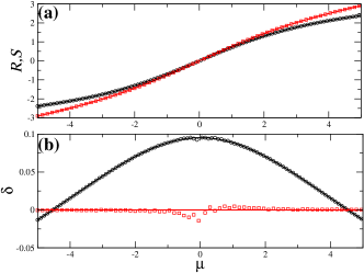
Figure 3: Individual based numerical simulation of Gaussian selection and the response to it as described in figure 2 ; The selection function here is a Gaussian $\exp\left((z-\mu)^{2}/2\sigma_{W}^{2}\right)$. (a) The mean phenotype of the selected $S=E(Z_{w})$ (red squares) and the progeny $R=E(Z_{1})$ (black circles) as a function of the optimum phenotype $\mu$. (b) the deviation $\delta$ from their theoretical values of the of the realized heritability $R/S-h^{2}$ (black circles) and and its alternative form $R^{\prime}/S^{\prime}-j^{2}$ (red squares) as a function of $\mu$. Continuous traits represent theoretical values obtained from eqs (3,4)

If the selection function, and the distributions of genotype and environment factors are all Gaussian functions, the standard and alternative breeder’s equation can be combined, which leads to a simple linear relation

$$S = \alpha\mu$$ (20)

$$R = \alpha h^{2}\mu$$ (21)

where $\alpha=(j^{2}-1)/(j^{2}-h^{2})$. Relations (20,21) can be used as a test for normal distribution of the genotype.

The alternative equation (19) is not in contradiction with Fisher’s fundamental theorem and does not predict evolution independently of genetic variance. Both $R^{\prime}$ and $S^{\prime}$ are dependent on the genetic variance, as can be seen in the general equations (3-4) ; the coefficient of the linear equation (19) relating them however is free of genetic variance. Consider for example the extreme case where there is no genetic variance ($\sigma_{A}=0$). The distribution of the breeding value then becomes a Dirac’s delta function $p_{0}(y)=\delta(y)$ and the value of $R$ and $S$ are readily obtained from equations (3-4):

$$R = 0$$ (22)

$$S = \mu\frac{\sigma_{E}^{2}}{\sigma_{W}^{2}+\sigma_{E}^{2}}$$ (23)

Therefor $R^{\prime}=-\mu$, $S^{\prime}=-\mu/j^{2}$ and equation (19) is verified trivially.

Selection on multiple traits.

The results of the above sections are naturally generalized to selection on multiple traits. Consider the vectors of parental breeding values $\mathbf{y}_{0}=(y_{1},y_{2},...y_{N})$, environmental effects $\mathbf{e}=(e_{1},...,e_{N})$ and their phenotype $\mathbf{z}_{0}=\mathbf{y}_{0}+\mathbf{e}$ , to which a selection function $W(\mathbf{z})$ is applied. Using the same notations as in the previous sections, we find without difficulty that

$$\bar{\mathbf{z}}_{1} = \int_{\mathbb{R}^{N}\times\mathbb{R}^{N}}\mathbf{y}p_{0}(\mathbf{y})W(\mathbf{z})f(\mathbf{z}-\mathbf{y})d\mathbf{y}d\mathbf{z}$$

$$\bar{\mathbf{z}}_{w} = \int_{\mathbb{R}^{N}\times\mathbb{R}^{N}}\mathbf{z}p_{0}(\mathbf{y})W(\mathbf{z})f(\mathbf{z}-\mathbf{y})d\mathbf{y}d\mathbf{z}$$

As before, using Fourier Transforms, these relations transform into

$$\bar{\mathbf{z}}_{1} = \frac{i}{2\pi}\int_{\mathbb{R}^{N}}\tilde{W}^{*}(\mathbf{k})\left(\nabla\tilde{p}_{0}(\mathbf{k})\right)\tilde{f}(\mathbf{k})d^{M}\mathbf{k}$$

$$\bar{\mathbf{z}}_{w} = \frac{i}{2\pi}\int_{\mathbb{R}^{N}}\tilde{W}^{*}(\mathbf{k})\nabla\left(\tilde{p}_{0}(\mathbf{k})\tilde{f}(\mathbf{k})\right)d^{M}\mathbf{k}$$

where $\nabla$ is the gradient operator: $\nabla f=(\partial f/\partial x_{1},...\partial f/\partial x_{N})$. We see again that $\mathbf{\bar{z}}_{1}$ and $\mathbf{\bar{z}}_{w}$ are linearly related if

$$\tilde{p}_{0}(\mathbf{k})\left(\nabla\tilde{f}(\mathbf{k})\right)=A\left(\nabla\tilde{p}_{0}(\mathbf{k})\right)\tilde{f}(\mathbf{k})$$

where $A$ is a constant matrix. The linear relation is automatically satisfied if both $p_{0}$ and $f$ follow a Gaussian distribution

$$p_{0}(\mathbf{y}) \propto \exp\left(-\frac{1}{2}\mathbf{y}^{T}G^{-1}\mathbf{y}\right)$$

$$f(\mathbf{x}) \propto \exp\left(-\frac{1}{2}\mathbf{x}^{T}E^{-1}\mathbf{x}\right)$$

where $G$ and $E$ are the covariance matrices for the genotype and environmental effects. Defining $P=G+E$ as the phenotype covariance matrix, it is straightforward to show that in this case $A=EG^{-1}$ and therefore Lande (1979)

$$\bar{\mathbf{z}}_{1}=GP^{-1}\mathbf{\bar{z}}_{w}$$

which is the usual breeder’s equation for multiple traits. We stress that the limitation of this relation is the same as that of the scalar version : it relies on the normal distribution of the genotype. On the other hand, if the selection function $W(\mathbf{z})$ is Gaussian

$$W(\mathbf{z})\propto\exp\left(-\frac{1}{2}(\mathbf{z}-\mathbf{\mu)}^{T}\Omega^{-1}(\mathbf{z-}\mu)\right)$$

the arguments of the previous section II can be repeated and lead to the generalization of the alternative vectorial breeder’s equation (19)

$$\bar{\mathbf{z}}_{1}-\mathbf{\mu}=(\Omega+E)\Omega^{-1}(\mathbf{\bar{z}}_{w}-\mathbf{\mu})$$

which, in analogy with equation (19) we write as

$$\mathbf{R}^{\prime}=(\Omega+E)\Omega^{-1}\mathbf{S}^{\prime}$$

III Discussion & Conclusion.

The breeder’s equation is a cornerstone of quantitative genetics and appears as a fundamental equation in all the important textbooks of this field Lynch and Walsh (1998); Falconer and Mackay (1995); Crow and Kimura (2009). It is widely used in artificial selection Lush (1943); Hill and Kirkpatrick (2010); its usage in natural selection was popularized by Lande Lande (1976) when he formalized the main idea of phenotypic evolution and it is now commonly used in many articles based on Lande’s work (see for example Manna et al. (2011); Svardal et al. (2011); Hansen et al. (2011) ). The mathematical foundation of this equation rests upon the hypothesis that the breeding value is normally distributed. This hypothesis is plausible for a continuous trait in a population not subject to selection (see however Appendix/Segregation density function). The normal distribution of the breeding value is more fragile in populations subjected to selection on this trait Turelli and Barton (1990), as the genotype of selected parents is given by (eq. 7)

$$p_{w}(y)=p_{0}(y).W^{\dagger}(y)/\bar{W}$$

where $W^{\dagger}(y)$ is the genotype fitness function defined by eq. (8). Even if $p_{0}(y)$ were Gaussian, the very act of multiplying it by an arbitrary function makes $p_{w}(y)$, and hence $p_{1}(y)$ non-Gaussian. Therefore after the first round of selection, the normal distribution hypothesis of parental genotype cannot be sustained. Turelli and Barton Turelli and Barton (1994) have shown that for the infinitesimal model, the non-normality may not have large effects on the predictions of the breeder’s equation, but they argued that when the number of loci is limited the discrepancy can grow much larger. Of course even $p_{0}(y)$ cannot be assumed to be Gaussian if different breeds are crossed to constitute the parental generation, which happens in artificial selection and in natural selection when gene flow from nearby patches is important.

The breeding value is not an observable quantity. The fitness or selection function $W(z)$ is more quantifiable and many authors have considered a Gaussian selection function. In artificial selection, it dates back at least to the work of Lush Lush (1943), p140). In natural selection, it is used by most authors as a model for stabilizing selection. If Gaussian selection is used to evolve a population, then the alternative breeding equation (19) we derived is more precise and predictive and rests on more robust mathematical grounds while retaining the same simplicity of the standard breeder’s equation. Note that the analysis of this article is not restricted to the infinitesimal model, but applies to all inheritance processes involving purely additive genetic effects. The alternative breeder’s equation generalizes to selection on multiple traits in a similar way to the standard breeder’s equation and can therefore be incorporated in the “adaptive landscape” formalism Arnold et al. (2001) with the same ease.

In conclusion, we believe that in all cases where Gaussian selection functions are used to evolve a population, the alternative breeder’s equation we develop above is a useful alternative approach to the standard method.

Acknowledgment.

I thank Jarrod Hadfield for discussions and comments on earlier drafts that helped to improve the manuscript. I am also grateful to M. Vallade, E. Geissler, O. Rivoire and A. Dawid for careful reading of the manuscript and fruitful discussions. The author declares to have no conflict of interest.

IV Appendix.

Fourier Transforms and convolutions.

The Fourier Transform (FT) of a function $f(x)$ is defined here as Byron and Fuller [1992]

$$\tilde{f}(k)=\mbox{TF}\left[f(x)\right]=\int_{-\infty}^{+\infty}f(x)e^{-ikx}dx$$

where $i^{2}=-1$. The main properties of FT we use here are (i) Parseval’s theorem

$$\int_{-\infty}^{+\infty}f^{*}(x)g(x)dx=\frac{1}{2\pi}\int_{-\infty}^{+\infty}\tilde{f}^{*}(k)\tilde{g}(k)dk$$

where $a^{*}$ stands for the conjugate complex of $a$ ; (ii) the derivation property

$$i\frac{d}{dk}\tilde{f}(k)=\int_{-\infty}^{+\infty}xf(x)e^{-ikx}dx=\mbox{TF}\left[xf(x)\right]$$

(iii) the convolution property

$$\mbox{FT}\left[(f*g)(x)\right]=\mbox{FT}\left[f(x)\right].\mbox{FT}\left[g(x)\right]=\tilde{f}(k).\tilde{g}(k)$$

Based on the above properties, and the fact that all the above functions are real i.e., for example $W^{*}(z)=W(z)$, we see that relation (3) can be written as

$$\iint_{\mathbb{R}^{2}}yp_{0}(y)W^{*}(z)f(z-y)dydz = \int_{\mathbb{R}}W^{*}(z)\left(yp_{0}*f\right)(z)dz$$

$$= \frac{i}{2\pi}\int_{\mathbb{R}}\tilde{W}^{*}(k)\tilde{p}^{\prime}(k)\tilde{f}(k)dk$$

where we have used the fact (i) that $\mbox{FT}\left[yp_{0}(y)\right]=i\tilde{p}^{\prime}(k)$ ; (ii) FT transforms a convolution product into a simple product in reciprocal space and (iii) Parseval’s theorem.

The same set of rules leads to

$$\iint_{\mathbb{R}^{2}}zp_{0}(y)W^{*}(z)f(z-y)dydz = \int_{\mathbb{R}}W^{*}(z)z\left(p_{0}*f\right)(z)dz$$

$$= \frac{i}{2\pi}\int_{\mathbb{R}}\tilde{W}^{*}(k)\frac{d}{dk}\left[\tilde{p}(k)\tilde{f}(k)\right]dk$$

Note that we can exchange the order of integration on $y$ and $z$, write the first integral as a convolution product on functions of $z$ and proceed to the second integral by using the Fourier Transform on $y$. For $R$, we have

$$\iint_{\mathbb{R}^{2}}yp_{0}(y)W(z)f(z-y)dydz = \int_{\mathbb{R}}p_{0}^{*}(y)y\left(W*f\right)(y)dy$$

$$= \frac{i}{2\pi}\int_{\mathbb{R}}\tilde{p}^{*}(k)\frac{d}{dk}\left[\tilde{W}(k)\tilde{f}(k)\right]dk$$

and for $S$ we get

$$\iint_{\mathbb{R}^{2}}zp_{0}(y)W(z)f(z-y)dydz = \int_{\mathbb{R}}p_{0}^{*}(y)\left(zW*f\right)(y)dy$$

$$= \frac{i}{2\pi}\int_{\mathbb{R}}\tilde{p}^{*}(k)\tilde{W}^{\prime}(k)\tilde{f}(k)dk$$

The translation property of Fourier Transforms

$$\mbox{FT}\left[W_{c}(z-\mu)\right]=e^{-ik\mu}\mbox{FT}\left[W_{c}(z)\right]$$

was used in the derivation of the functional lags (17,18).

Finally, note that the FT of a Gaussian is a Gaussian :

$$\mbox{FT}\left[\frac{1}{\sqrt{2\pi}s}\exp(-x^{2}/(2s^{2})\right]=\exp\left(-s^{2}k^{2}/2\right)$$

Parent-Offspring regression.

The derivation of the breeder’s equation sometimes uses the parent-offspring regression coefficient as an intermediateLynch and Walsh [1998], Nagylaki [1992]. The linear regression between parent and offspring phenotype however is based on the same assumption of normal distribution of genotype and environmental factors.

The probability density of observing the phenotype $z^{\prime}$ in the offspring and $z_{a},z_{b}$ in the parents is

$$p(z^{\prime};z_{a},z_{b}) = \iint_{\mathbb{R}^{2}}p(y_{a})f(z_{a}|y_{a})p(y_{b})f(z_{b}|y_{b})$$

$$L\left(y_{1}-(y_{a}+y_{b})/2\right)f(z^{\prime}|y_{1})dy_{1}dy_{a}dy_{b}$$

and the conditional expectation of $z^{\prime}$ given $z$ is

$$E(z^{\prime}|z_{a},z_{b})=\int_{z^{\prime}\in I}z^{\prime}p(z^{\prime},z)dz^{\prime}/\int_{z^{\prime}\in I}p(z^{\prime},z)dz^{\prime}=F(z_{a},z_{b})$$

It is not difficult to check that the function $F(z_{a},z_{b})$ is a linear function of its argument

$$F(z_{a},z_{b})=b(z_{a}+z_{b})/2$$

if both the genotype and environment factors obey a normal distribution, in which case, the linearity coefficient is indeed $b=\sigma_{A}^{2}/(\sigma_{A}^{2}+\sigma_{E}^{2})$. However, even if the parental generation follows a normal distribution, the selected parents do not (equation 7) and the use of parent-offspring regression poses even more of a problem than the direct method.

Segregation density function.

Let $p_{0}(y)$ be the distribution of breeding value in the parental generation. In the absence of selection, after recombination-segregation, the distribution of breeding value in the progeny is

$$p_{1}(y)=\iint_{\mathbb{R}^{2}}p_{0}(y_{a})p_{0}(y_{b})L\left(y-(y_{a}+y_{b})/2\right)dy_{a}dy_{b}$$ (24)

where the function $L(y)$ is the segregation density function capturing the inheritance process of the breeding value Karlin [1979]. $L(y)$ is a probability density function and in the absence of epistasis and dominance effect, its average is zero : $\int_{\mathbb{R}}yL(y)dy=0$. In the infinitesimal model framework, $L(y)$ is a normal distribution of variance $\sigma_{A}^{2}/2$ . However, any distribution probability $L(y)$ will lead to a stable, although not necessarily normal, probability distribution of breeding values after few round of reproduction. Let us set the origin of the breeding value at its average in the parental distribution, i.e. $\int_{\mathbb{R}}yp_{0}(y)dy=0$. In Fourier space relation (24) is

$$\tilde{p}_{1}(k)=\tilde{p}_{0}^{2}(k/2)\tilde{L}(k)$$

and after $n$ rounds of reproduction,

$$\tilde{p}_{n}(k)=\tilde{p}_{0}^{2^{n}}(k/2^{n})\prod_{i=0}^{n-1}\tilde{L}^{2^{i}}(k/2^{i})$$

As both $p_{0}(y)$ and $L(y)$ are probability distribution functions of zero mean, we have

$$\tilde{p}_{0}(0) = \tilde{L}(0)=1$$

$$\tilde{p}^{\prime}_{0}(0) = \tilde{L^{\prime}}(0)=0$$

and therefore

$$\tilde{p}^{\prime\prime}_{n}(0)=\frac{1}{2^{n}}\tilde{p}^{\prime\prime}_{0}(0)+(2-\frac{1}{2^{n-1}})\tilde{L}^{\prime\prime}(0)$$

Let $V=\int_{\mathbb{R}}y^{2}L(y)dy$ . We see then that

$$\mbox{Var}(Y_{n})=\frac{1}{2^{n}}\mbox{Var}(Y_{0})+(2-\frac{1}{2^{n-1}})V$$

So the variance of the breeding values converges fast to twice the variance of the segregation density function. The distribution function $p_{n}(y)$ however converges to a normal distribution only if $L(y)$ is normal.

Individual based numerical simulations.

The numerical simulations are performed with the Matlab (Mathwork inc.) program. $N$ individuals (usually $10^{6}$ ) are generated and stored in a genotype table $y0$, the genotype $y0(i)$ of individual $i$ is drawn from a given zero-mean distribution. A table $\xi 0$ of the same size is drawn from a normal distribution $\mathcal{N}(0,\sigma_{E})$ and table $z0=y0+\xi 0$ is then generated: $u0=[y0,z0]$ constitutes the parental genotype-phenotype table. For a given fitness function $W(z)\leq 1$, a survival table $r$ of size $N$, drawn from a uniform distribution $\mathcal{U}(0,1)$ is generated. A logical filter selects elements in $u0$ if $W\left(z0(i)\right)\geq r(i)$. The selected elements constitute the new table $uw=[yw,zw]$ of size $N1$. A table $\xi 1$ of size $N1$ is drawn again from a normal distribution $\mathcal{N}(0,\sigma_{E})$ and the phenotype of the offspring is computed by $z1=yw+\xi 1$. The various distributions can now be computed from these tables. The selection differential and the response are computed in the same way, $R=\mbox{mean}(z1)$ and $S=\mbox{mean}(zw)$.

The above procedure is the core program and is used in other programs, for example to measure $R$ and $S$ as a function of the selection function translation.

References

- Arnold et al. [2001] Stevan J. Arnold, Michael E. Pfrender, and Adam G. Jones. The adaptive landscape as a conceptual bridge between micro- and macroevolution. Genetica, 112-113:9–32, 2001. ISSN 0016-6707. URL http://dx.doi.org/10.1023/A:1013373907708.
- Bulmer [1985] M.G. Bulmer. The Mathematical Theory of Quantitative Genetics. Oxford University Press, USA, 1985.
- Byron and Fuller [1992] Frederick W. Byron and Robert W. Fuller. Mathematics of Classical and Quantum Physics. Dover Publications Inc, 1992.
- Crow and Kimura [2009] J. F. Crow and M. Kimura. An Introduction to Population Genetics Theory. The Blackburn Press, Cal, 2009.
- Falconer and Mackay [1995] D. S. Falconer and T. F. C. Mackay. Introduction to Quantitative Genetics. Longman; 4 edition, 1995.
- Gavrilets and Hastings [1995] S. Gavrilets and A. Hastings. Dynamics of polygenic variability under stabilizing selection, recombination, and drift. Genet Res, 65:63–74, 1995.
- Geyer and Shaw [2008] Ch.J. Geyer and R. G. Shaw. Commentary on lande-arnold analysis. Technical Report 670, School of Statistics/University of Minnesoto, 2008.
- Gienapp and al. [2008] P. Gienapp and al. Climate change and evolution: disentangling environmental and genetic responses. Mol Ecol, 17:167–178, 2008. doi: 10.1111/j.1365-294X.2007.03413.x. URL http://dx.doi.org/10.1111/j.1365-294X.2007.03413.x.
- Haldane [1954] J.B.S. Haldane. The measurement of natural selection. Caryologia, 6(Suppl.):480?487, 1954.
- Hansen et al. [2011] T. F. Hansen, C. Pelabon, and D. Houle. Heritability is not evolvability. Evol. Biol., 38:258–277, 2011. doi: 10.1007/s11692-011-9127-6.
- Heywood [2005] J. S. Heywood. An exact form of the breeder’s equation for the evolution of a quantitative trait under natural selection. Evolution, 59:2287–2298, 2005.
- Hill and Kirkpatrick [2010] W. G. Hill and M. Kirkpatrick. What animal breeding has taught us about evolution. Ann. Rev. Ecol. Evol. Syst., Vol 41, 41:1–19, 2010. doi: 10.1146/annurev-ecolsys-102209-144728.
- Karlin [1979] S. Karlin. Models of multifactorial inheritance .1. multivariate formulations and basic convergence results. Theoretical Population Biology, 15:308–355, 1979. doi: 10.1016/0040-5809(79)90044-3.
- Karlin and Liberman [1979a] S. Karlin and U. Liberman. Central equilibria in multilocus systems .1. generalized non-epistatic selection regimes. Genetics, 91(4):777–798, 1979a.
- Karlin and Liberman [1979b] S. Karlin and U. Liberman. Representation of non-epistatic selection models and analysis of multilocus hardy-weinberg equilibrium configurations. Journal of Mathematical Biology, 7(4):353–374, 1979b. doi: 10.1007/BF00275154.
- Kimura and Crow [1978] M. Kimura and J. F. Crow. Effect of overall phenotypic selection on genetic change at individual loci. PNAS, 75:6168–6171, 1978.
- Kruuk [2004] L. E. B. Kruuk. Estimating genetic parameters in natural populations using the ‘animal model’. Phil. Trans. R. Soc. London. Series B, 359:873–890, 2004. doi: 10.1098/rstb.2003.1437. URL http://rstb.royalsocietypublishing.org/content/359/1446/873.abstract.
- Lande [1976] R. Lande. Natural-selection and random genetic drift in phenotypic evolution. Evolution, 30:314–334, 1976. doi: 10.2307/2407703.
- Lande [1979] R. Lande. Quantitative genetic-analysis of multivariate evolution, applied to brain - body size allometry. Evolution, 33:402–416, 1979. doi: 10.2307/2407630.
- Lande and Arnold [1983] R. Lande and S. J. Arnold. The measurement of selection on correlated characters. Evolution, 37:1210–1226, 1983. doi: 10.2307/2408842.
- Lewontin [1964] R. C. Lewontin. The interaction of selection and linkage. ii. optimum models. Genetics, 50:757–782, 1964. URL http://www.ncbi.nlm.nih.gov/pmc/articles/PMC1210693/pdf/757.pdf.
- Lush [1943] J. L. Lush. Animal breeding plans. The Iowa State College Press, 1943. URL http://www.archive.org/details/animalbreedingpl032391mbp.
- Lynch and Walsh [1998] M. Lynch and B. Walsh. Genetics and anaysis of quantitative traits. Sinauer Associates, 1998.
- Manna et al. [2011] F. Manna, G. Martin, and T. Lenormand. Fitness landscapes: An alternative theory for the dominance of mutation. Genetics, 189:923–U303, 2011. doi: 10.1534/genetics.111.132944.
- Nagylaki [1992] T. Nagylaki. Rate of evolution of a quantitative character. PNAS, 89:8121–8124, 1992.
- Pemberton [2010] J. M. Pemberton. Evolution of quantitative traits in the wild: mind the ecology. Phil. Trans. R. Society B, 365:2431–2438, 2010. doi: 10.1098/rstb.2010.0108.
- Pigliucci [2006] M. Pigliucci. Genetic variance-covariance matrices: A critique of the evolutionary quantitative genetics research program. Biol. & Phil., 21:1–23, 2006. doi: 10.1007/s10539-005-0399-z.
- Pigliucci and Schlichting [1997] M. Pigliucci and C. D. Schlichting. On the limits of quantitative genetics for the study of phenotypic evolution rid a-1389-2010. Acta Biotheoretica, 45:143–160, 1997. doi: 10.1023/A:1000338223164.
- Raj and van Oudenaarden [2008] A. Raj and A. van Oudenaarden. Nature, nurture, or chance: stochastic gene expression and its consequences. Cell, 135:216–226, 2008. doi: 10.1016/j.cell.2008.09.050. URL http://dx.doi.org/10.1016/j.cell.2008.09.050.
- Roff [2000] D. Roff. The evolution of the g matrix: selection or drift? Heredity, 84:135–142, 2000.
- Slatkin [1970] M. Slatkin. Selection and polygenic characters. Proceedings of the National Academy of Sciences of the United States of America, 66:87–93, 1970. doi: 10.1073/pnas.66.1.87.
- Svardal et al. [2011] H. Svardal, C. Rueffler, and J. Hermisson. Comparing environmental and genetic variance as adaptive response to fluctuating selection. Evolution, 65:2492–2513, 2011. doi: 10.1111/j.1558-5646.2011.01318.x.
- Turelli and Barton [1990] M. Turelli and N. H. Barton. Dynamics of polygenic characters under selection. Theoretical Population Biology, 38(1):1–57, August 1990. doi: 10.1016/0040-5809(90)90002-D.
- Turelli and Barton [1994] M. Turelli and N. H. Barton. Genetic and statistical-analyses of strong selection on polygenic traits - what, me normal. Genetics, 138(3):913–941, November 1994.
- Visscher and al. [2008] P. M. Visscher and al. Heritability in the genomics era - concepts and misconceptions rid b-3198-2012. Nat. Rev. Genetics, 9:255–266, 2008. doi: 10.1038/nrg2322.
- Wright [1920] S. Wright. The relative importance of heredity and environment in determining the piebald pattern of guinea-pigs. PNAS, 6:320–332, 1920. URL http://www.pnas.org/content/6/6/320.short.
- Wright [1935] S. Wright. The analysis of variance and the correlations between relatives with respect to deviations from an optimum. J. Genet., 30:243–256, 1935.
- Zhang and Hill [2010] X-S Zhang and W. G. Hill. Change and maintenance of variation in quantitative traits in the context of the price equation. Theor.Pop. Biol., 77:14 – 22, 2010. ISSN 0040-5809. doi: 10.1016/j.tpb.2009.10.004. URL http://www.sciencedirect.com/science/article/pii/S0040580909001142.