Quantum phases of the Shastry-Sutherland Kondo lattice:
implications for the global phase diagram of heavy fermion metals

Abstract

Considerable recent theoretical and experimental efforts have been devoted to the study of quantum criticality and novel phases of antiferromagnetic heavy-fermion metals. In particular, quantum phase transitions have been discovered in heavy-fermion compounds with geometrical frustration. These developments have motivated us to study the competition between the RKKY and Kondo interactions on the Shastry-Sutherland lattice. We determine the zero-temperature phase diagram as a function of magnetic frustration and Kondo coupling within a slave-fermion approach. Pertinent phases include the valence bond solid and heavy Fermi liquid. In the presence of antiferromagnetic order, our zero-temperature phase diagram is remarkably similar to the global phase diagram proposed earlier based on general grounds. We discuss the implications of our results for the experiments on Yb₂Pt₂Pb and related compounds.

Geometrical frustration in insulating quantum antiferromagnets can lead to a variety of quantum phases, such as valence bond solids (VBS) and quantum spin liquids Balents . Recent studies have discovered intriguing properties in a growing list of metallic systems with local magnetic moments residing on frustrated lattices. In these heavy fermion compounds, the interplay of Kondo screening and magnetic frustration may give rise to entirely new ground states and quantum phase transitions Si . For example, the compounds Yb₂Pt₂Pb Kim and CePd_1-xNi_xAl Fritsch have spin-$1/2$ local moments located on the Shastry-Sutherland and Kagome lattices respectively. Likewise, both YbAgGe Morosan and YbAl₃C₃ Khalyavin feature triangular lattices. All these compounds show an enhanced specific heat coefficient, implying a large effective mass and the presence of the Kondo effect.

General theoretical considerations of the competition between Kondo and RKKY interactions have led to a proposal for the global phase diagram of heavy fermion metals as a function of frustration or quantum fluctuations ($G$), and the Kondo coupling ($J_{K}$) Si2 ; Coleman ; see Fig. 1(a). This phase diagram incorporates not only antiferromagnetic (AF) order, but also the physics of Kondo destruction LCP ; JPCM ; Senthil . From the Kondo-destroyed antiferromagnetic phase (AF_S), the transition to the heavy fermi liquid phase (P_L) could take place directly (type I), via the spin-density-wave phase (AF_L) (type II), or through the Kondo-destroyed paramagnetic phase ($P_{S}$) (type III). The heavy fermion compounds CeCu_6-xCu_x, YbRh₂Si₂ and CeRhIn₅ have shown strong evidence for realizing the type I transition Schroder ; Friedeman ; Shishido ; Park06 . CePd₃Si₂₀, which is cubic and therefore would have a smaller $G$, has properties consistent with a type II transition Custers12 . Geometrical frustration is expected to enhance the quantum fluctuation parameter $G$, raising the prospect of realizing a type III transition. There is a recent surge of heavy-fermion materials that appear to be suitable for exploring this large-$G$ portion of the global phase diagram. In particular, Yb₂Pt₂Pb and its homologues such as Ce₂Pt₂Pb Kim , featuring the geometrically-frustrated Shastry-Sutherland lattice, may involve an intermediate VBS P_S phase.

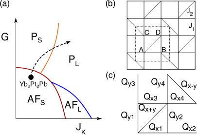
Figure 1: (color online). (a) Proposed global phase diagram of heavy fermion metals. Here, AF_S and AF_L refer to antiferromagnetic states without or with static Kondo screening. P_L is the paramagnetic heavy Fermi liqud, and P_S refers to a paramagnetic phase without static Kondo screening. Adapted from Ref. Si2 . We have sketched the proposed trajectory of Yb₂Pt₂Pb under magnetic field tuning. (b) Shastry-Sutherland lattice, denoting the Heisenberg exchange couplings $J_{1}$ on all the horizontal and vertical bonds, and $J_{2}$ along the diagonals. The unit cell is the dashed square, containing four sites $A,B,C,D$. (c) The bond singlet parameters.

In this work, we study the effect of frustration on the Kondo-Heisenberg model by considering it on the Shastry-Sutherland lattice (SSL) Shastry , as illustrated in Fig. 1(b). The Hamiltonian is defined as

$$H=\sum_{(i,j),\sigma}t_{ij}(c_{i\sigma}^{{\dagger}}c_{j\sigma}+\mathrm{h.c.})+J_{K}\sum_{i}{\bf S}_{i}\cdot{\bf s}_{i}^{c}+\sum_{(i,j)}J_{ij}{\bf S}_{i}\cdot{\bf S}_{j}$$ (1)

where $(i,j)$ denote the nearest neighbors (NN) and next nearest neighbors (NNN) on the SSL as shown in Fig. 1(b). The NN and NNN tight binding parameters for the conduction electrons, denoted by $c_{i\sigma}$, are $t_{1}$ and $t_{2}$, respectively. The spins of the conduction electrons are ${\bf s}_{i}^{c}=c_{i\alpha}^{{\dagger}}(\bm{\sigma}_{\alpha\beta}/2)c_{i\beta}$ at site $i$, where $\bm{\sigma}_{\alpha\beta}$ are the Pauli spin matrices. They are coupled to spin-$1/2$ local moments, ${\bf S}_{i}$, through an antiferromagnetic Kondo coupling $J_{K}$. We have explicitly included the RKKY interactions, incorporating $J_{1}$ and $J_{2}$, the NN and NNN terms respectively [Fig. 1(b)]. The degree of frustration is measured by the ratio $G=J_{2}/J_{1}$. We represent the local moments using fermionic spinons Auerbach , $f_{i\sigma}$ such that ${\bf S}_{i}=f_{i\alpha}^{{\dagger}}(\bm{\sigma}_{\alpha\beta}/2)f_{i\beta}$ with a constraint $\sum_{\sigma}f_{i\sigma}^{{\dagger}}f_{i\sigma}=1$ at each lattice site. The spin-$1/2$ Heisenberg model on the SSL was extensively studied (e.g., Refs. Shastry ; Chung ; Lauchli ; Miyahara ). For $J_{2}/J_{1}>2$, it possesses an exact VBS ground state, where singlets form across each disconnected diagonal bond Shastry . Whereas for small $J_{2}/J_{1}$, the model has an AF ground state Chung ; Lauchli . The transition between these two states has not been completely determined  Chung ; Lauchli . The model in the presence of Kondo coupling was studied in some detail by Bernhard et al. Bernhard , and was also discussed qualitatively Coleman . As we will discuss, our work here reports the first complete analysis of the relevant phases, and this is essential both in realizing the global phase diagram and in shedding light on the experimentally observed PKS phase.

Large-$N$ limit: Generalizing the spin symmetry from $SU(2)$ to $SU(N)$, we arrive at $H=\sum_{(i,j),\sigma}t_{ij}(c_{i\sigma}^{{\dagger}}c_{j\sigma}+\mathrm{h.c.})-J_{K}/N\sum_{i}:B_{i}^{{\dagger}}B_{i}:-\sum_{(i,j)}(J_{ij}/N):D_{ij}^{{\dagger}}D_{ij}:$ where $B_{i}=\sum_{\sigma}c_{i\sigma}^{{\dagger}}f_{i\sigma}$, $D_{ij}=\sum_{\sigma}f_{i\sigma}^{{\dagger}}f_{j\sigma}$. The sum now runs over $\sigma=1,\dots,N$, and the constraint becomes $\sum_{\sigma}f_{i\sigma}^{{\dagger}}f_{i\sigma}=N/2$. We have also used $:\dots:$ to denote normal ordering. The large-$N$ mean field Hamiltonian can be expressed as:

$$H_{MF} = E-\sum_{(i,j),\sigma}(Q_{ij}^{*}f^{{\dagger}}_{i\sigma}f_{j\sigma}+\mathrm{h.c.})+\sum_{i,\sigma}\lambda_{i}f^{{\dagger}}_{i\sigma}f_{i\sigma}$$

$$+ \sum_{(i,j),\sigma}t_{ij}(c^{{\dagger}}_{i\sigma}c_{j\sigma}+\mathrm{h.c.})-\sum_{i,\sigma}(b_{i}^{*}c^{{\dagger}}_{i\sigma}f_{i\sigma}+\mathrm{h.c.}).$$

We have used a Hubbard-Stratonovich transformation decoupling $B_{i}$ and $D_{ij}$ in the Kondo singlet and resonating valence bond (RVB) channels respectively  Senthil ; Coleman2 , and the constraint is enforced by $\lambda_{i}$. The constant term is $E/N=\sum_{i}\left(|b_{i}|^{2}/J_{K}-\lambda_{i}/2\right)+\sum_{(i,j)}|Q_{ij}|^{2}/J_{ij}$. The Kondo parameter $Nb_{i}=J_{K}\langle B_{i}\rangle$ can be taken to be real by absorbing its phase into the constraint field $\lambda_{i}$ Read , whereas the RVB parameters $NQ_{ij}=J_{ij}\langle D_{ij}\rangle$ are in general complex.

We solve Eq. (LABEL:eqn:Hmf) by using a four-site unit cell, where each site is labeled by $i\rightarrow({\bf r},X)$, with $X=A,B,C,D$ marking the sublattice [see Fig. 1(b)], and ${\bf r}$ specifying a unit cell. We introduce Fourier transforms per sublattice Dodds as $c_{{\bf r}X\sigma}=1/\sqrt{N_{u}}\sum_{{\bf k}}e^{-i{\bf k}\cdot({\bf r}+\bm{\delta}_{X})}c_{{\bf k}X\sigma}$, where $\bm{\delta}_{X}$ points to each sub lattice $X$ from sub-lattice $A$. Keeping the full generality of the four-site unit cell we introduce sublattice dependent Kondo parameters and constraint fields $b_{X},\lambda_{X}$, and use ten complex RVB parameters $Q_{ij}$ as shown in Fig. 1(c). These parameters are determined by solving the saddle-point equations self-consistently (see supplementary material supp ). We consider the metallic case $0<n_{c}<1$, where $n_{c}=\frac{1}{4N_{u}}\sum_{i,\sigma}\langle c^{\dagger}_{i\sigma}c_{i\sigma}\rangle$ is the filling of the conduction band.

The zero temperature phase diagram is shown in figure 2. Without loss of generality, we have chosen $t_{1}/t_{2}=1.0$ and $n_{c}=0.5$ for Figs. 2 and 3. For small Kondo coupling and a large $J_{2}/J_{1}$ ratio, a VBS ground state arises for which only $Q_{x+y}=Q_{x-y}$ are nonzero. The singlet bonds are the same as in the pure Heisenberg model in the Shastry-Sutherland lattice at large $J_{2}/J_{1}$, and we label it as SSL-VBS. This solution does not break any symmetry of the SSL.

Keeping $J_{K}/t_{1}$ small and decreasing $J_{2}/J_{1}$, we find a first order transition at $J_{2}/J_{1}=1$ from the SSL-VBS to a plaquette VBS (P-VBS) ground state where only $Q_{x2}=Q_{x4}=Q_{y1}=Q_{y2}$ are nonzero. The P-VBS ground state breaks a reflection symmetry about either of the diagonal bonds in the the SSL. It is degenerate with the conventional VBS on the square lattice with only $Q_{x1}=Q_{x4}$ being nonzero.

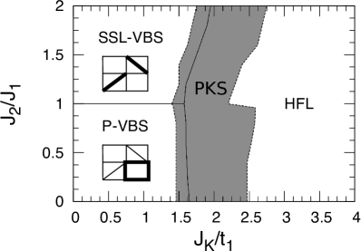
Figure 2: (color online). Large-$N$ phase diagram as a function of frustration ($J_{2}/J_{1}$) and Kondo coupling ($J_{K}/t_{1}$), for a metallic filling $n_{c}=0.5$. The phases are described in the main text. The solid lines represent first-order transitions, and the dashed lines surrounding the grey area locate the boundaries of the intermediate phases that exhibit partial Kondo screening (PKS).

For a large Kondo coupling we find a heavy Fermi liquid (HFL) ground state, which has a nonzero Kondo parameter $b_{A}=b_{B}=b_{C}=b_{D}$. The singlet bond parameters are also nonzero: $Q_{xi}=Q_{yi}$, for $i=1-4$ and $Q_{x+y}=Q_{x-y}$. We also obtain $\lambda_{A}=\lambda_{B}=\lambda_{C}=\lambda_{D}$, so the solution does not break any symmetry of the SSL. Here, we find that each $Q_{ij}$ acquires a finite phase $Q_{ij}=|Q_{ij}|e^{i\phi_{ij}}$. Correspondingly, we define a gauge independent flux through the triangular and square plaquettes as $\Phi_{\triangle}=\sum_{\triangle}\phi_{ij}(\mathrm{mod}\,\,2\pi)$ and $\Phi_{\square}=\sum_{\square}\phi_{ij}(\mathrm{mod}\,\,2\pi)$, respectively, where the summation is over the bonds around a plaquette. For the range of fillings $0<n_{c}\lesssim 0.75$, we find $\Phi_{\triangle}=\pi$ and $\Phi_{\square}=0$, whereas for $0.75\lesssim n_{c}<1$ we obtain $\Phi_{\triangle}=0$ and $\Phi_{\square}=0$. The finite flux through each triangular plaquette is a consequence of the spinons acquiring a finite kinetic energy from their hybridization with the conduction-electron band; we can therefore consider this as a hybridization induced flux phase. However, even though the flux through each triangular plaquette is $\pi$, the total flux through each square plaquette is still zero (mod. $2\pi$); the flux does not affect the electronic band structure in the HFL phase.

We now turn to the transition among the two VBS phases and the HFL phase. Restricting the solution to these three states, we obtain the phase boundary in Fig. 2 and the mean field parameters shown in Fig. 3(a). Unexpectedly, when considering the general solution we find a number of intermediate states that break the lattice symmetry, in the region shown as the grey shaded area in Fig. 2. In some cases, for example the intermediate phase between the SSL-VBS phase and the HFL phase we find a PKS state: some (half) of the moments in the unit cell are still locked into valence bonds, while the other spins are Kondo screened. This is discussed in detail in the supplementary material supp . Tuning $t_{1}/t_{2}$ only affects the location of the phase boundary; a smaller ratio of $t_{1}/t_{2}$ makes the transition between each VBS phase and the HFL phase occur for smaller values of $J_{K}/t_{1}$.

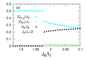
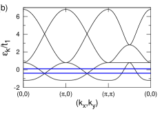
Figure 3: (color online). (a) The bond and Kondo singlet parameters at a fixed ratio $J_{2}/J_{1}=2.0$ as a function of $J_{K}$, displaying a first order transition from the SSL-VBS to the HFL phase. We show the three dimensionless independent quantities for the solution that breaks no lattice translational symmetry. Band structure along high symmetry directions in the reduced Brillouin zone in the SSL-VBS phase with $J_{K}=0$ and $J_{2}/J_{1}=2.0$ (b) and in the HFL phase with $J_{K}=2.1t_{1}$ and $J_{2}/J_{1}=2.0$ (c). The thick blue lines are the gapped spinon dispersion in the SSL-VBS phase.

Magnetism at $N=2$: We now incorporate long range AF order into our approach. To do so we decouple the Heisenberg term into two distinct channels, but we no longer have access to the large-$N$ limit and are restricted to $N=2$. In keeping with the generalized procedure of Hubbard-Stratonovich decouplings NG.book , and similar to reference Senthil , we rewrite the Heisenberg term in Eq. (1) as follows: $J_{ij}{\bf S}_{i}\cdot{\bf S}_{j}=xJ_{ij}{\bf S}_{i}\cdot{\bf S}_{j}+(1-x)J_{ij}{\bf S}_{i}\cdot{\bf S}_{j}$; the term proportional to $x$ is treated within the RVB decoupling described previously. The additional term is decoupled in terms of Néel order: $(1-x)J_{ij}{\bf S}_{i}\cdot{\bf S}_{j}=(1-x)J_{ij}(2{\bf M}_{i}\cdot{\bf S}_{j}-{\bf M}_{i}\cdot{\bf M}_{j})$, where ${\bf M}_{i}=\langle{\bf S}_{i}\rangle$. We consider the Néel ground state with an ordering wave vector ${\bf Q}=(\pi/a,\pi/a)$ . This AF order corresponds to ${\bf M}_{A}={\bf M}_{D}=-{\bf M}_{C}=-{\bf M}_{B}={\bf M}$ within the four site unit cell. In the absence of a Kondo coupling, $J_{K}=0$, the phase diagram of the Heisenberg model as a function of $x$ and $J_{2}/J_{1}$ is presented in the supplementary material supp .

The phase diagram at $J_{K}=0$ provides the physical basis for choosing the parameter $x$. Within our fermonic representation, classical AF order arises at $x=0$, corresponding to a full ordered magnetic moment $|{\bf M}|=1/2$. The ground state wave function of the true quantum AF state is known to contain considerable RVB correlations Dagatto , suggesting a choice of $x>1/2$. Indeed, for the nearest neighbor Heisenberg model ($J_{K}=0$ and $J_{2}=0$) we find a quantum AF phase as a self consistent solution for $x$ in the range $0.67\leq x<0.8125$, which has a lower free energy than the classical Néel state ($Q_{xi}=Q_{yi}=0$). This state, is a free energy local minimum, and taken as a candidate of the true Néel ground state. The quantum AF phase has finite RVB parameters $Q_{xi}=Q_{yi}$ for $i=1-4$, which reduce the ordered moment $|{\bf M}|<1/2$. Incorporating fluctuations further will reduce the free energy even more, making the AF phase the true ground state in the limit $J_{2}/J_{1}\ll 1$. Here we present the results for $x=0.7$. The phases and the overall profile of the phase diagram are not sensitive to the choice of $x$ in the range $0.67\leq x<0.8125$, as discussed in the supplementary material supp .

The resulting phase diagram is given in Fig. S6, for parameters $n_{c}=0.5$ and $t_{1}/t_{2}=1$. We have restricted the solutions to states that do not break any lattice symmetries. For small $J_{K}/t_{1}$ and tuning the ratio of $J_{2}/J_{1}$, we find a first order transition from the AF phase to the SSL-VBS phase. For small $J_{2}/J_{1}$, and tuning the Kondo coupling, the AF phase has a continuous transition note into a spin density wave (SDW) phase characterized by the onset of Kondo screening: $b_{A}=b_{B}=b_{C}=b_{D}$ increases continuously from zero with nonzero values of ${\bf M}$, $Q_{xi}=Q_{yi}$ for $i=1-4$ and $Q_{x+y}=Q_{x-y}$. Upon increasing $J_{K}$ further, there is a first order transition from the SDW phase into the HFL phase with ${\bf M}=0$.

Our results demonstrate a rich interplay between Kondo and RKKY interactions. In addition to the AF order and its suppression, there is also the competition between the Kondo effect and VBS order in the magnetically-disordered region. In the notation of Fig. 1(a), we associate Kondo hybridization ($b\neq 0$) with a large Fermi surface (subscript $L$) and Kondo destruction ($b=0$) with a small Fermi surface (subscript $S$). The phase diagram we have calculated, Fig. S6, represents a remarkable realization of the global phase diagram that had been advanced on qualitative considerations Si2 ; Coleman . It will be instructive to study Kondo lattice models in other geometrically frustrated cases, for example Kagome lattices (pertinent to CePd_1-xNi_xAl Fritsch ) and triangular lattices (relevant to YbAgGe Morosan and YbAl₃C₃ Khalyavin ), and explore the generality of the global phase diagram. Compared to those cases, the Kondo model on the SSL has the main advantage that the magnetically frustrated regime is accessible by a large-$N$ approach.

Several remarks are in order. First, in the phase diagram of Fig. S6, we find a line of direct transitions from AF_S to P_L. However, whether this is a line of transitions or a single point is sensitive to the model parameters in our approach and for $x=0.75$ we find the transition collapsing to a single point (see the supplementary material supp ). It is important to consider how further quantum fluctuations will affect the topology of the phase diagram in Fig. S6. Recently, insights have been gained from calculations on a quantum impurity model incorporating local quantum fluctuations Nica ; within an extended dynamical mean field context LCP , the results of Ref. Nica imply this direct transition to be a line in the phase diagram.

Second, due to an even number of spins per unit cell, the spinon bands are either empty or completely full Coleman . Hence the volume of the Fermi surface will not change when the system goes from the SSL-VBS to the HFL phase. Nonetheless, the topology of the Fermi surfaces reflects the incorporation ($L$) or absence ($S$) of the Kondo resonances in the Fermi volume and can be different for the two cases. We show the Fermi surfaces for $n_{c}=0.5$ in the supplementary material supp .

Third, it is instructive to compare our results to those of Ref. Bernhard, . Where there is overlap, the results of that work and ours are largely consistent. We are able to draw substantially new implications by studying the competitions of all the phases pertinent to the global phase diagram, including the $AF_{L}$ phase. Furthermore, our work has also uncovered PKS phases. In a similar vein, we note that the Shastry-Sutherland Kondo lattice was also considered in Ref. Coleman, , with a particular focus on possible superconducting pairings. The implications of our study for superconductivity is an intriguing issue, but is beyond the scope of the present work.

Figure 4: Phase diagram of the Shastry-Sutherland Kondo lattice incorporating magnetic order for a metallic filling $n_{c}=0.5$. Thin (thick) lines represent first order (continuous note ) transitions.

The systematic nature of our results is important not only for generating insights into the global phase diagram, but also to drawing implications for experiments in heavy-fermion metals. Our phase diagram in Fig. S6 opens up a trajectory from the AF_S to the HFL phase via a sequence of quantum phase transitions that passes through a VBS, $P_{S}$ phase. This result has implications for Yb₂Pt₂Pb, where experiments Kim appear to have realized such a sequence of transitions [see figure 1(a)].

In addition, we have provided evidence for intermediate, partially Kondo screened phases in metallic cases. This type of phase has also been discussed in a variational quantum Monte Carlo approach in Kondo insulator settings  Motome . In this regard, it is intriguing that experiments on the metallic CePd_1-xNi_xAl Fritsch have suggested that the frustration in this material is not large enough to yield a spin liquid, but instead leads to a ground state where some of the magnetic moments form long range AF order, while the others are completely screened by the Kondo effect.

In conclusion, we have studied the global phase diagram in the prototypical geometrically-frustrated Shastry-Sutherland Kondo lattice. Our work represents the first concrete calculation in which all four phases, AF_S, AF_L, P_S, and P_L appear in a single zero-temperature phase diagram. Our results have elucidated the rich variety of quantum phases and their transitions in heavy-fermion metals, and provide new insights into the puzzling experimental observations recently made in geometrically frustrated heavy fermion metals.

Acknowledgements: We would like to acknowledge useful discussions with D. T. Adroja, M. Aronson, C. H. Chung, P. Coleman, S. Kirchner, A. Nevidomskyy, and E. Nica. This work was supported in part by the NSF Grant No. DMR-1309531, the Robert A. Welch Foundation Grant No. C-1411, the Alexander von Humboldt Foundation and the East-DeMarco fellowship (JHP). The majority of the calculations have been performed on the Shared University Grid at Rice funded by NSF under Grant EIA-0216467, and a partnership between Rice University, Sun Microsystems, and Sigma Solutions, Inc.. Q.S.  also acknowledges the hospitality of the the Karlsruhe Institute of Technology, the Aspen Center for Physics (NSF Grant No. 1066293), and the Institute of Physics of Chinese Academy of Sciences.

Supplementary Material
Quantum phases of the Shastry-Sutherland Kondo lattice:
implications for the global phase diagram of heavy fermion metals

J. H. Pixley, Rong Yu and Qimiao Si

I Numerical Method to Solve the Self-Consistent Equations

In this work, we minimize the ground-state energy with respect to the self-consistent parameters $Q_{ij}$, $b_{X}$, and $\lambda_{X}$ by solving the coupled non-linear equations. To solve the equations efficiently, we apply the Broyden’s mixing method Broyden65 ; NumRecp07 ; Johnson88 , which has been widely used in density functional theory (DFT) MarksLuke08 ; Baran , in dynamical mean-field theory Zitko09 , and in other contexts of correlated electron problems Yunoki08 ; Yu13 . In general, the method solves the self-consistent equations $\bm{X}=\bm{F}[\bm{X}]$ iteratively with a set of initial values of the parameters $\bm{X}^{(0)}_{\mathrm{in}}$. At the $m$-th iteration, a new set of the parameters is obtained via

$$\bm{X}^{(m)}_{\mathrm{out}}=\bm{F}[\bm{X}^{(m)}_{\mathrm{in}}].$$ (S1)

The input of the next iteration is constructed from

$$\bm{X}^{(m+1)}_{\mathrm{in}}=\bm{X}^{(m)}_{\mathrm{in}}-\bm{B}^{(m)}(\bm{X}^{(m)}_{\mathrm{out}}-\bm{X}^{(m)}_{\mathrm{in}}),$$ (S2)

where $\bm{B}^{(m)}$ is an approximation to the inverse Jacobian matrix of the non-linear equations at the $m$-th iteration. The Broyden’s method provides a scheme to update the approximate inverse Jacobian $\bm{B}^{(m)}$ at each iteration such that good convergence is obtained Broyden65 ; NumRecp07 ; Johnson88 .

To achieve the global minimum of the ground-state energy, we have done a random search of initial conditions in the parameter space. The typical number of the $\bm{X}^{(0)}_{\mathrm{in}}$ configurations used in the calculation is $10^{3}$. For each given initial condition, a Broyden mixing is performed; when convergence is approached, the corresponding ground-state energy is recorded. The global minimum of the ground-state energy is then obtained by comparing the energies for different configurations.

II Intermediate Phases and the Effect of Model Parameters

Here we present the full Large-N phase diagram for the metallic SS Kondo lattice, focusing in particular on the intermediate phases sketched in Fig. 2 of the main text. We consider tight binding parameters $t_{1}=t_{2}=1$, and a conduction electron filling $n_{c}=0.5$. We find a series of intermediate states that break the lattice symmetry within the unit cell. In particular we find four intermediate states labelled with different colors in Fig. S1: blue (1), green (2), red (3) and grey (4).

We first consider the blue region (1), which is the most physically relevant intermediate phase because it occurs in the transition region between the SSL-VBS and HFL phases. Here, we find a phase with partial Kondo screening defined as $b_{A}=b_{D}>0$, $b_{B}=b_{C}=0$, with $Q_{x-y}\gg Q_{x+y}>0$. The local moments on sublattices A and D are screened by the Kondo effect, whereas those on the $B$ and $C$ sub-lattices are locked into a VBS singlet. Turning next to the green region (2), we find a square plaquette RVB phase with Kondo screening, defined by $b_{A}=b_{D}>b_{B}=b_{C}>0$, $Q_{x-y}>Q_{x+y}>0$, $Q_{x1}=Q_{y1}=Q_{x3}=Q_{y2}$ and $Q_{x2}=Q_{y3}=Q_{x4}=Q_{y4}$. In this phase, plaquette valence bonds form on each square plaquette that contains a $J_{2}$ bond. The red region (3) describes a phase where the RVB parameters are in a “kite” phase, and the local moments are screened. It is defined by $b_{A}=b_{D}>b_{B}=b_{C}$, $Q_{x+y}\neq Q_{x-y}$, $Q_{x1}=Q_{y1}$, $Q_{x2}=Q_{y3}$, $Q_{x3}=Q_{y2}$, and $Q_{x4}=Q_{y4}$. Lastly, we come to the grey region (4), which corresponds to a spin-Peierls phase with partial Kondo screening. Here, $b_{A}=b_{B}\neq 0$, $b_{C}=b_{D}=0$ with $Q_{x3}\neq 0$; all the other parameters vanish.

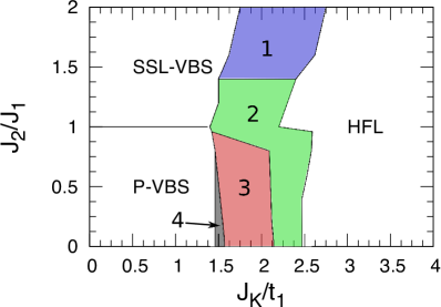
Figure S1: Full large-N phase diagram of the SS Kondo lattice, for $t_{2}=t_{1}$ and $n_{c}=0.5$. The phases are described in the text.

Figure S2: Phase diagram of the SS Kondo lattice incorporating magnetic order using $x=0.75$, while keeping $t_{2}=t_{1}$ (a) and for $x=0.70$ with $t_{2}=0$ (b). In both cases, the conduction electron filling, $n_{c}=0.5$, is unchanged from before. The thin (thick) lines represent first order (continuous) transitions.

We now turn the effect of changing model parameters on the global phase diagram. We first consider choosing a different value of $x=0.75$ (see the main text for the definition of $x$) while keeping $t_{1}/t_{2}=1$ and $n_{c}=0.5$. This choice of $x$ is still in the range over which a quantum antiferromagnetic phase arises (see below, Fig. S6). Separately, we consider keeping $x=0.70$ but setting $t_{2}=0$, with $t_{1}/J_{1}=4.0$ and $n_{c}=0.5$; this allows us to study the effect of the conduction-electron band dispersion (cf. Figs. S4 and S5). Interestingly, for both cases we find the line of transitions between AF_S and HFL collapse to a point. Therefore, whether the transition between AF_S and HFL is a line or a single point is a question that needs to be addressed beyond the mean field level, for example within an extended dynamical mean field approach. The key point, however, is that the overall profile of the global phase diagram is robust against these changes of parameters.

Figure S3: (a) Fermi Surface corresponding to the band structure in Fig. 3(b) of the main text, in the VBS phase. Here, $J_{2}/J_{1}=2$, $J_{K}/t_{1}=2.1$. Since the spinon bands are gapped, this corresponds to the band structure of the conduction electron dispersion alone, defined on the SSL with $t_{1}/t_{2}=1$ and $n_{c}=0.5$; (b) Fermi Surface corresponding to the band structure in Fig. 3(c) of the main text, in the HFL phase. The bare parameters are the same as in (a). Note that the Fermi volume does not change from (a) to (b), due to the even number of spins per unit cell as described in the main text.

To explore further the robustness of our results against the change of the conduction-electron dispersion, we also discuss the effect of an additional tight binding parameter $t_{3}$, which connects every next nearest neighbor that is not connected via $t_{2}$. Just like tuning $t_{2}/t_{1}$ away from $1$, any finite $t_{3}$ will introduce a curvature to the region of the flat band; this flat portion existed for $t_{2}/t_{1}=1$ (and $t_{3}=0$), along the $k_{x}=k_{y}$ direction in the Brillouin zone and away from the Fermi energy, as shown in Fig. 3(b) in the main text. We find that tuning the ratio of $t_{3}/t_{1}$ can change the degree to which the intermediate PKS phases occur. The region of the intermediate phases that break the lattice symmetry within the unit cell narrows for increasing $t_{3}/t_{1}$, and can even be completely eliminated for a large $t_{3}/t_{1}$ ratio. Again, the overall profile of the global phase diagram is robust against the change of $t_{3}/t_{1}$.

We close this subsection by showing the Fermi surfaces of the SSL-VBS and HFL phases, both for the case $t_{2}=t_{1}$ and $n_{c}=0.5$ (Figs. S3(a) and (b), respectively) and for $t_{2}=0$ and $n_{c}=0.5$ (Figs. S4 and S5, respectively).

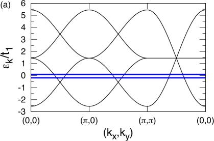
Figure S4: (a) Band structure in the VBS phase when the diagonal hopping vanishes, $t_{2}/t_{1}=0$, and for $J_{2}/J_{1}=1.6$, $J_{K}/t_{1}=0$ and $n_{c}=0.5$. The parameter $t_{1}=1.0$ sets the unit of energy. The blue lines are the gapped spinon bands. The Fermi energy is at $\epsilon_{k}/t_{1}=0$; (b) The corresponding Fermi surface.

Figure S5: (a) Band structure in the HFL phase, for parameters as in Fig. S4. The fermi energy is also at $\epsilon_{k}/t_{1}=0$; (b) The corresponding Fermi surface.

III Magnetic Phase Diagram

Finally, we discuss the Heisenberg model in the absence of any Kondo coupling in our approach, when both the RVB correlations and Néel order are incorporated and the self consistent solutions with the lowest free energy are determined. The region for the candidate quantum Néel phase, as described in the main text, is also considered as a self consistent solution. The resulting phase diagram is shown in Fig. S6, where both the P-VBS and SSL-VBS phases have been described in the main text. The classical Néel state (Classical AFM) is defined as ${\bf M}_{A}={\bf M}_{D}=-{\bf M}_{B}=-{\bf M}_{C}>0$, with all the other parameters equal to zero. Here the order parameter retains the full classical moment. We find the candidate quantum Néel phase, with ${\bf M}_{A}={\bf M}_{D}=-{\bf M}_{B}=-{\bf M}_{C}>0$ and $Q_{xi}=Q_{yi}\neq 0$, $i=1-4$ to be a self consistent solution only in the range $0.67\leq x<0.8125$. The nonzero RVB singlet parameters cause a reduced value for the ordered moment. This is shown as the magenta region in Fig. S6, where the boundary of the region at a finite ratio of $J_{2}/J_{1}$ marks the transition to the SSL-VBS phase. For a judicious choice of $x$ in the range $0.6<x<0.67$ we find the transition from the classical AFM phase to the SSL-VBS has an intermediate P-VBS phase similar to what is found in exact diagonalization studies (see reference [20] in the main text). We remark that for $x=0.5$, which treats Néel and VBS order on equal footing, we find the location of the transition from the classical AFM phase to the SSL-VBS to be $(J_{2}/J_{1})_{c}=1.35$ which is close to the value obtained from a variety of other methods (see reference [21] in the main text).

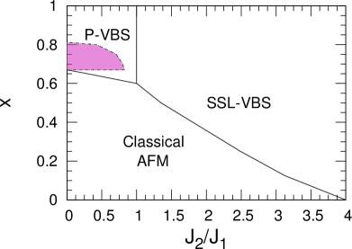
Figure S6: The phase diagram of the Heisenberg model in the slave-fermion approach. The parameter $x$ and the phases are described in the main text.

References

- (1) L. Balents, Nature 464, 199 (2010).
- (2) Q. Si and F. Steglich, Science 329, 1161 (2010).
- (3) M. S. Kim and M. C. Aronson, Phys. Rev. Lett. 110, 017201 (2013); M. S. Kim, M. C. Bennet, and M. C. Aronson, Phys. Rev. B 77, 144425 (2008); M. S. Kim and M. C. Aronson, J. Phys.: Condens. Matter 23 164204 (2011).
- (4) V. Fritsch, N. Bagrets, G. Goll, W. Kittler, M. J. Wolf, K. Grube, C.-L. Huang, and H. v. Löhneysen, arXiv:1301.6062 (2013).
- (5) J. K. Dong, Y. Tokiwa, S. L. Bud’ko, P. C. Canfield, and P. Gegenwart, Phys. Rev. Lett. 110, 176402 (2013); S. L. Bud’ko, E. Morosan, P. C. Canfield, Phys. Rev. B 71, 054408 (2005).
- (6) D. D. Khalyavin, D. T. Adroja, P. Manuel, A. Daoud-Aladine, M. Kosaka, K. Kondo, K. A. McEwen, J. H. Pixley and Q. Si, Phys. Rev. B 87, 220406(R) (2013).
- (7) Q. Si, Physica B 378, 23 (2006); Phys. Status Solidi B 247, 476 (2010).
- (8) P. Coleman and A. Nevidomskyy, J. Low. Temp. Phys. 161, 182 (2010).
- (9) Q. Si, S. Rabello, K. Ingersent and J. L. Smith, Nature 413, 804 (2001).
- (10) P. Coleman, C. Pépin, Q. Si, and R. Ramazashvili, J. Phys.: Conden. Matt. 13, R723-R738 (2001).
- (11) T. Senthil, M. Vojta, and S.Sachdev, Phys. Rev. B 69, 035111 (2004).
- (12) A. Schröder, G. Aeppli, R. Coldea, M. Adams, O. Stockert, H. v. Löhneysen, E. Bucher, R. Ramazashvili, and P. Coleman, Nature 407, 351 (2000).
- (13) S. Friedemann, N. Oeschler, S. Wirth, C. Krellner, C. Geibel, F. Steglich, S. Paschen, S. Kirchner, and Q. Si, PNAS 107, 14547-14551 (2010).
- (14) H. Shishido, R. Settai, H. Harima and Y. Ōnuki, J. Phys. Soc. Jpn. 74, 1103 (2005).
- (15) T. Park, F. Ronning, H. Q. Yuan, M. B. Salamon, R. Movshovich, J. L. Sarrao and J. D. Thompson, Nature 440 65 (2006).
- (16) J. Custers, K.-A. Lorenzer, M. Müller, A. Prokofiev, A. Sidorenko, H. Winkler, A. M. Strydom, Y. Shimura, T. Sakakibara, R. Yu, Q. Si, and S. Paschen, Nature Materials 11, 189 (2012).
- (17) B. S. Shastry and B. Sutherland, Physica B 108, 1069 (1981).
- (18) D. P. Arovas and A. Auerbach, Phys. Rev. B 38 316 (1988).
- (19) C. H. Chung, J. B. Marston and S. Sachdev, Phys. Rev. B 64 134407 (2001).
- (20) A. Lauchli, S. Wessel, and M. Sigrist Phys. Rev. B 66, 014401 (2002).
- (21) S. Miyahara and K. Ueda, J. Phys.: Condens. Matter 15, R327 (2003).
- (22) B. H. Bernhard, B. Coqblin, and C. Lacroix, Phys. Rev. B 83, 214427 (2011).
- (23) P. Coleman and N. Andrei, J. Phys.: Condens. Matter 1, 4057 (1989).
- (24) N. Read, D. M. Newns and S. Doniach, Phys. Rev. B 30, 3841 (1984)
- (25) S. Furukawa, T. Dodds and Y. B. Kim, Phys. Rev. B 84, 054432 (2011).
- (26) See Supplemental Material.
- (27) J. W. Negele and H. Orland, Quantum Many-Particle Systems, Westview Press (1998).
- (28) A. Auerbach, Interacting electrons and quantum magnetism, Springer (1994).
- (29) E. Dagotto and A. Moreo, Phys. Rev. B 38, 5087(R) (1988).
- (30) We are not able to discern between a continuous and a very weakly first order transition.
- (31) E. M. Nica, K. Ingersent, J. X. Zhu and Qimiao Si, Phys. Rev. B 88, 014414 (2013).
- (32) Y. Motome, K. Nakamikawa, Y. Yamaji and M. Udagawa, Phys. Rev. Lett. 105 036403 (2010).

References

- (1) C. G. Broyden, Math. Comput. 19, 577 (1965).
- (2) W. H. Press, S. A. Teukolsky, W. T. Vetterling, and B. P. Flannery, Numerical Recipies: The Art of Scientific Computing, 3rd ed. (Cambridge University Press, New York, 2007).
- (3) D. D. Johnson, Phys. Rev. B 38, 12807 (1988).
- (4) L. D. Marks and D. R. Luke, Phys. Rev. B 78, 075114 (2008).
- (5) A. Baran et al., Phys. Rev. C 78, 014318 (2008).
- (6) R. Žitko, Phys. Rev. B 80, 125125 (2009).
- (7) S. Yunoki, E. Dagotto, S. Costamagna, and J. A. Riera, Phys. Rev. B 78, 024405 (2008).
- (8) R. Yu, P. Goswami, Q. Si, P. Nikolic, and J.-X. Zhu, Nat. Commun. 4, 2783 (2013).