New Radial Abundance Gradients for NGC 628 and NGC 2403

Danielle A. Berg¹¹affiliation: Department of Astronomy, University of Minnesota, 116 Church St. SE, Minneapolis, MN 55455; berg@astro.umn.edu; skillman@astro.umn.edu , Evan D. Skillman¹¹affiliation: Department of Astronomy, University of Minnesota, 116 Church St. SE, Minneapolis, MN 55455; berg@astro.umn.edu; skillman@astro.umn.edu , Donald R. Garnett, Kevin V. Croxall²²affiliation: Ohio State University, 140 West 18th Avenue, Columbus, OH 43210; croxall.5@osu.edu , Andrew R. Marble³³affiliation: National Solar Observatory, 950 N Cherry Ave, Tucson, AZ 85719; amarble@nso.edu , J.D. Smith⁴⁴affiliation: Ritter Astrophysical Observatory, University of Toledo, Toledo, OH 43606, USA; jd.smith@utoledo.edu , Karl Gordon⁵⁵affiliation: Space Telescope Science Institute, 3700 San Martin Drive, Baltimore, MD 21218, USA; kgordon@stsci.edu , Robert C. Kennicutt, Jr.⁶⁶affiliation: Institute of Astronomy, University of Cambridge, Madingley Road, Cambridge CB3 0HA, UK; robk@ast.cam.ac.uk ⁷⁷affiliation: Steward Observatory, University of Arizona, Tucson, AZ 85721

galaxies: abundances - galaxies: spiral - galaxies: evolution

Motived by recent ISM studies, we present high quality MMT and Gemini spectroscopic observations of H II regions in the nearby spiral galaxies NGC 628 and NGC 2403 in order to measure their chemical abundance gradients. Using long-slit and multi-object mask optical spectroscopy, we obtained measurements of the temperature sensitive auroral lines [O III] $\lambda 4363$ and/or [N II] $\lambda 5755$ at a strength of 4 $\sigma$ or greater in 11 H II regions in NGC 628 and 7 regions in NGC 2403. These observations allow us, for the first time, to derive an oxygen abundance gradient in NGC 628 based solely on “direct” oxygen abundances of H II regions: 12 + log(O/H) = (8.43 $\pm$ 0.03) + (-0.017 $\pm$ 0.002) $\times{R_{g}}$ (dex/kpc), with a dispersion in log(O/H) of $\sigma$ = 0.10 dex, from 14 regions with a radial coverage of $\sim$ 2-19 kpc. This is a significantly shallower slope than found by previous “strong-line” abundance studies. In NGC 2403, we derive an oxygen abundance gradient of 12 + log(O/H) = (8.48 $\pm$ 0.04) + (-0.032 $\pm$ 0.007) $\times{R_{g}}$ (dex/kpc), with a dispersion in log(O/H) of $\sigma$ = 0.07 dex, from 7 H II with a radial coverage of $\sim$ 1-10 kpc.

Additionally, we measure the N, S, Ne, and Ar abundances. We find the N/O ratio decreases with increasing radius for the inner disk, but reaches a plateau past $R_{25}$ in NGC 628. NGC 2403 also has a negative N/O gradient with radius, but we do not sample the outer disk of the galaxy past $R_{25}$ and so do not see evidence for a plateau. This bi-modal pattern measured for NGC 628 indicates dominant contributions from secondary nitrogen inside of the $R_{25}$ transition and dominantly primary nitrogen farther out. As expected for $\alpha$ -process elements, S/O, Ne/O, and Ar/O are consistent with constant values over a range in oxygen abundance.

1 INTRODUCTION

H II regions can be used to study absolute and relative abundances in the interstellar medium (ISM) of galaxies. Aller (1942) and Searle (1971) were the first to infer radial gradients in excitation across the disks of spiral galaxies. Since then, numerous studies have shown that, typically, spiral galaxies have radial abundance gradients in the sense of decreasing absolute abundances with increasing galactocentric radius. This trend was first measured in our own galaxy by Shaver et al. (1983) and was confirmed by observations of other nearby spiral galaxies (e.g., Pagel & Edmunds, 1981; Shields, 1990). Thus, spiral galaxies in the nearby universe with low inclinations offer the opportunity to measure chemical abundances and subsequently compare these abundances with variations in physical conditions.

The dust properties of the ISM in spiral galaxies (such as the dust-to-gas ratio and the abundance of polycyclic aromatic hydrocarbons (PAHs)) are known to show systematic radial variations. Previous studies have investigated the correlation between PAH emission and metallicity, and found that PAH emission drops below a critical metallicity of 12+log(O/H) $\approx$ 8.0 in nearby dwarf galaxies (e.g., Engelbracht et al., 2005, 2008; Marble et al., 2010). These works suggest that metallicity may play a role in PAH processing, and thus PAH abundance relative to total dust content, but other factors such as star formation and/or the local radiation field density affect the excitation of those molecules. Other studies have supported the hypothesis that grain formation and modification is affected by local metallicity (e.g., Smith et al., 2007; Sandstrom et al., 2012).

Whether or not this result is universal is key to understanding PAH behavior in the ISM and requires a greater pool of reliable data. Smith et al. (2005) carried out a successful Spitzer observing campaign with deep, spatially resolved, low-resolution spectral maps from 5 to 38 microns in three nearby galaxies (M 101, NGC 628, and NGC 2403) to address these questions. Since the physical conditions in the ISM are likely important to the star formation process and play a role in the composition, conditions, and size distribution of dust grains, understanding the connection between chemical abundances and the physical conditions in the ISM is fundamental to understanding star formation and galaxy evolution. Thus we are motivated to measure reliable direct abundance gradients for NGC 628 and NGC 2403; these results are being incorporated into the PAH studies of Sandstrom et al. (2013) and Smith et al. (2013).

Detailed direct abundance studies exist for only a handful of spiral galaxies. For example, direct H II region abundances have been successfully measured for 20 high signal-to-noise H II region spectra in M 101 by Kennicutt et al. (2003). However, only two H II region auroral line detections exist in the literature for NGC 628 (Castellanos et al., 2002), and so no direct oxygen abundance gradient has ever been reported. The H II regions of NGC 2403 have been studied by Garnett et al. (1997), but there were concerns about the linearity of the detector used.

In order to place gradients on the same scale for comparison amongst galaxies, reliable and consistent derivations of abundances are needed (see, e.g., Moustakas et al., 2010). However, the vast majority of nebular abundance measurements for H II regions in spiral galaxies are based upon “strong-line” observations which lack a “direct” measurement of the electron temperature in the ionized gas. The conversion of these strong-line observations into chemical abundances can be very uncertain and biased (Kennicutt et al., 2003; Bresolin, 2007; Yin et al., 2007; Pérez-Montero & Contini, 2009; Berg et al., 2011), limiting their ability to provide meaningful comparisons between different galaxies. Therefore, a “direct” measurement of the electron temperature - typically derived from the ratio of auroral to collisionally excited lines - is needed for each H II region. Throughout the remainder of the paper, abundances determined in this fashion will be referred to as direct abundances. Since the auroral lines become exponentially weaker with decreasing temperature (increasing abundance), observations become increasingly challenging at higher metallicities (small radii in spiral galaxies). Nonetheless, with large telescope apertures and efficient spectrographs, it is possible to determine accurate chemical abundance gradients for spiral galaxies (e.g., Kennicutt et al., 2003; Garnett et al., 2004; Bresolin et al., 2004; Bresolin, 2007; Bresolin et al., 2009, 2009; Bresolin, 2011; Zurita & Bresolin, 2012). Note that direct chemical abundances are not without problems (they assume a uniform temperature distribution, ignoring temperature fluctuations) and great progress is being made to overcome their limitations (e.g., Esteban et al., 2009; Peña-Guerrero et al., 2012; Nicholls et al., 2012). Even so, direct abundances do provide a stable and well understood scale by which to make comparisons between galaxies.

A major unresolved issue in H II region abundance studies is the importance of primary versus secondary production of nitrogen. Oxygen production is generally understood to be dominated by primary nucleosynthesis from massive stars and delivered early after a star formation event. Like oxygen, nitrogen can be produced by massive stars (and delivered early with the primary oxygen), as well as by intermediate mass stars (and delivered relatively later). Nitrogen can have both primary and secondary origins. Garnett (1990) found a relatively constant relationship in the N/O ratio versus O/H for low metallicity star-forming galaxies. At higher metallicities (i.e., 12+log(O/H) $\geq$ 8.0), secondary nitrogen production becomes increasingly significant, causing the average N/O to increase with O/H (Pagel, 1985). We can, therefore, use the radial relationship of N/O in spiral galaxies to determine which nucleosynthetic mechanisms are dominant.

A further goal of H II region spectroscopic studies it to measure $\alpha$ -element abundances as an observational constraint of the IMF and stellar nucleosynthesis models. Sulfur, neon, and argon are all $\alpha$ -process elements which are produced through hydrostatic burning and explosive nucleosynthesis: neon is a product of carbon burning, while sulfur and argon are produced during oxygen burning. In a comprehensive study of M33, Kwitter & Aller (1981) found that Ne, N, S, and Ar gradients followed that which they derived for oxygen. The stellar nucleosynthesis calculations of Woosley & Weaver (1995) modeled these trends, indicating the $\alpha$ -elements and oxygen are produced mainly in massive stars in a small mass range, and thus are expected to trace each other closely. In contrast to this viewpoint, Willner & Nelson-Patel (2002) derived a neon gradient that is significantly shallower than the oxygen gradient observed in M33. While sulfur is also traditionally assumed to have a constant S/O ratio (Garnett, 1989), some specific cases, such as the work of Vilchez et al. (1988) on M33, find a slower decline of sulfur than oxygen with radius. Thus additional $\alpha$ -element observations are needed to properly constrain stellar nucleosynthesis models.

Here we present new MMT and Gemini observations of H II regions in NGC 628 and NGC 2403, which allow improved measurements of their chemical abundance gradients. These allow us to estimate the abundance gradient of NGC 628 for the first time solely from direct abundances, and to improve the abundance gradient of NGC 2403 by increasing the number of H II regions with direct abundance measurements. In Section 2 we describe the MMT and Gemini observations and how we processed the spectra. Emission line measurements and abundance determinations are detailed in § 3, which allows the discussion of the oxygen abundance gradient in § 4.1, the nitrogen abundance gradient in § 4.2, and of the sulfur, neon, and argon abundances in § 4.3. Finally, we summarize our findings in § 5.

2 NEW SPECTROSCOPIC OBSERVATIONS

2.1 NGC 628 Spectra

NGC 628 (M 74) is a late-type giant spiral ScI galaxy with a systematic velocity of 656 km s ${}^{-1}$ . We adopt a distance of 7.2 Mpc (Van Dyk et al., 2006) and an inclination of $i\approx 5^{\circ}$ (Shostak & van der Kruit, 1984), with a resulting scale of 35 pc arcsec ${}^{-1}$ . The optical parameters of NGC 628 are listed in Table 1. NGC 628 is an excellent target due to its small inclination, extended structure, and undisturbed optical profile. The gas-phase oxygen abundance of NGC 628 has been previously studied using long-slit spectroscopy (e.g., Talent, 1983; McCall et al., 1985; Zaritsky et al., 1994; Ferguson et al., 1998; van Zee et al., 1998; Bresolin et al., 1999; Castellanos et al., 2002; Moustakas et al., 2010; Gusev et al., 2012; Cedrés et al., 2012), and integral field spectroscopy (e.g., Rosales-Ortega et al., 2011). Using strong-line abundances, these studies mostly found a constant gradient out to $R_{g}\sim 1.7\cdot R_{25}$ . In contrast, Rosales-Ortega et al. (2011) found a trimodal oxygen abundance gradient, where the innermost distribution is nearly flat, followed by a steep negative gradient out to $R_{25}$ , and another nearly constant gradient beyond the optical edge of the galaxy. Additionally, they found that the slope of the gradient depends strongly on the abundance calibrator used, concluding that this may be due to the potential for [N II]-based empirical indices to overestimate oxygen abundance at high N/O ratios and vice versa (see e.g., Pérez-Montero & Contini, 2009).

New MMT and Gemini observations were acquired in order to achieve high signal-to-noise (S $/$ N) spectra with the goal of detecting the faint [O III] $\lambda$ 4363 or [N II] $\lambda$ 5755 auroral lines at a strength of 4 $\sigma$ or higher. The Gemini observations were obtained from two multi-slit fields covering the inner parts of NGC 628 and these were supplemented by MMT observations of individual H II regions in the outer parts of NGC 628.

Intermediate-resolution spectra of H II regions in NGC 628 were obtained with the Gemini Multi-Object Spectrographs (GMOS; Hook et al., 2004) on the UT dates of 2006 September 21 and November 17. The multi-object mode of GMOS, which uses custom-designed, laser-milled masks, offers the possibility of obtaining spectra of many H II regions simultaneously. Pre-imaging in an H $\alpha$ filter was used to identify H II regions and determine accurate astrometry for the masks. H II regions were selected based on high H $\alpha$ surface brightness and a large radial coverage of the disk.

Two masks were observed in queue mode, one of the North-West corner of NGC 628, and one placed on the South-East corner. The NW and SE masks contained slits 1.5″ wide covering 7 and 8 different H II regions respectively. Slit lengths varied between 15-50″ depending on the the size of the targeted H II region and the proximity of other slits on the mask. Both blue and red spectra were obtained using a 600 line grating, giving a resolution of 0.45 Å per pixel and a full width half maximum resolution of $\approx 6$ Å. The red side additionally used the GG455_G0305 order blocking filter. Typical exposure times were 3 $\times$ 1675 seconds with the mask fixed to a position angle of zero, and the observations were obtained near transit. Observations were centered at 4600 Å, 4625 Å, and 4650 Å in the blue, and 6100 Å, 6125 Å, and 6150 Å in the red, to ensure full spectral coverage across the detector gaps.

The NGC 628 MMT observations were obtained with the Blue Channel spectrograph (Schmidt et al., 1989) on the UT dates of 2008 October 30-November 1, 2009 June 15-22, and 2010 January 11-12. Sky conditions varied, but data were only acquired during minimal cloud coverage and approximately arcsecond seeing. A 500 line grating, $1\arcsec$ slit, and UV-36 blocking filter were used, yielding an approximate dispersion of 1.2 Å per pixel, a full width at half maximum resolution of $\lesssim 3$ Å, and a wavelength coverage of 3690–6790 Å. The MMT and Blue Channel spectrograph combination provided the balance between sensitivity, resolution, and wavelength coverage conditions necessary to measure all emission lines relevant to oxygen abundance determinations. Bias frames, flat-field lamp images, and sky flats were taken each night. Multiple standard stars from Oke (1990) with spectral energy distributions peaking in the blue and containing minimal absorption were observed throughout the night using a 5 $\arcsec$ slit over a range of airmasses.

In each H II region, the slit center was aligned with H $\alpha$ emission such that the surface brightness over the area of the slit was maximized. Typically, three 1200 or 1800 second exposures were made for the MMT observations, with the slit at a fixed position angle which approximated the parallactic angle at the midpoint of the observation. This, in addition to observing the galaxies at airmasses less than 1.5, served to minimize the wavelength-dependent light loss due to differential refraction (Filippenko, 1982).

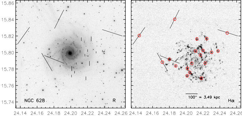
Finally, combined helium, argon, and neon arc lamps were observed at each pointing at the MMT, while copper-argon arc lamps were obtained at GEMINI for accurate wavelength calibration. Tables 2 and 3 list the log information for both the GMOS and MMT observations. Figure 1 shows the R-band continuum and H $\alpha$ continuum-subtracted images for NGC 628 (van Zee et al., in prep.), with slit positions from Tables 2 and 3 shown with black lines centered on red circles. The slit centers are marked in the H $\alpha$ image by red circles.

2.2 NGC 2403 Spectra

As a bright, nearby galaxy with a favorable inclination, NGC 2403 allows observations of the chemical composition throughout its disk. NGC 2403 is an intermediate luminosity, isolated spiral SABcd galaxy in the M81 Group. We adopt a distance of 3.16 Mpc (Jacobs et al., 2009) and an inclination of $\approx 60^{\circ}$ with a resulting scale of 15.3 pc arcsec ${}^{-1}$ . The optical parameters of NGC 2403 are listed in Table 1. Several strong-line spectroscopic studies relevant to our work exist for NGC 2403 (e.g., McCall et al., 1985; Fierro et al., 1986; van Zee et al., 1998). In contrast, Garnett et al. (1997) measured direct abundances using the [O III] $\lambda 4363$ , [S III] $\lambda 6312$ , and [O II] $\lambda$ 7320-7330 emission lines to determine the electron temperatures for 9 H II regions. Although the [O III] $\lambda$ 4363 line was detected at high confidence in these regions, there were some lingering concerns about the effects of the non-linearity of the IPCS detector that appear at moderately high count rates (Jenkins, 1987). Thus, checking on the reliability of the previous observations and increasing the number of measurements and radial coverage is desirable.

New MMT observations were acquired in order to achieve high signal-to-noise (S $/$ N) spectra with the goal of measuring direct abundances. Observations for NGC 2403 were acquired using the Blue Channel Spectrograph at the MMT on the UT dates of 2006 February 1-4. A setup similar to the NGC 628 observations was used, but the exposure time was varied corresponding to the surface brightness of the region. A 500 mm ${}^{-1}$ grating was used providing a 3650-6790 Å coverage. The H II regions of NGC 2403 have been identified and cataloged by Véron & Sauvayre (1965), Hodge & Kennicutt (1983), and Sivan et al. (1990). Targets were chosen to overlap with the sample from Garnett et al. (1997, here after referred to as G97) and also to improve the radial coverage. For five of the targets, a 832 mm ${}^{-1}$ grating was also used, providing additional wavelength coverage from 5495 to 7405 Å.

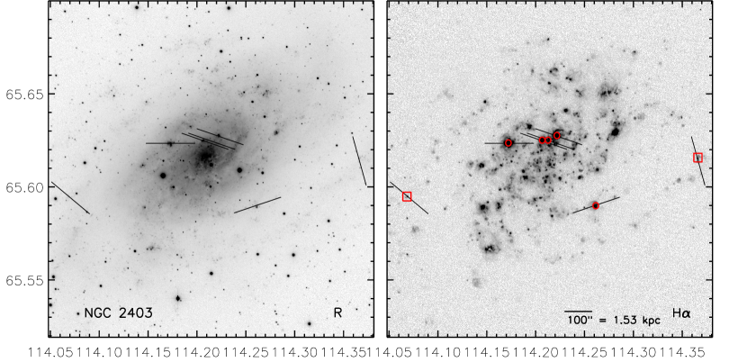
The log information for the NGC 2403 MMT observations are tabulated in Table 4. Figure 2 shows the R-band continuum and H $\alpha$ continuum-subtracted images for NGC 2403 (van Zee et al., in prep.), with central slit positions from Table 4 indicated by red circles for targets overlapping with the G97 sample and by red squares for new targets.

Refer to caption — Figure 1: R-band and continuum-subtracted H $\alpha$ images of NGC 628 (van Zee et al., in prep.). The lines represent the various slit positions observed at Gemini and the MMT. The central slit positions targeted H II regions and are indicated with red circles. See Tables 2 and 3 for more details.

Table 1: Properties of NGC 628 and NGC 2403

Property	NGC 628	NGC 2403
R.A.	01:36:41.747	07:36:51.400
Dec.	15:47:01.18	65:36:09.20
Type	ScI	SABcd
Adopted D (Mpc)	7.2 $\pm$ 1.0 ${}^{1}$	3.16 $\pm$ 0.07 ${}^{6}$
$m_{B}$ (mag)	9.95 ${}^{2}$	8.93 ${}^{2}$
Redshift	0.002192	0.000445
Inclination (degrees)	5 ${}^{3}$	60 ${}^{7}$
P.A. (degrees)	12 ${}^{4}$	126 ${}^{8}$
$R_{25}$ (arcmin)	5.25 ${}^{5}$	10.95 ${}^{5}$
$R_{25}$ (kpc)	10.95	10.07

Note. — Optical properties for NGC 628 and NGC 2403. Row 1 and 2 give the RA and Dec of the optical center in units of hours, minutes, and seconds, and decrees, arcminutes, and arcseconds respectively. Row 5 lists redshifts taken from the NASA/IPAC Extragalactic Database. Row 8 gives the optical radius at the $B_{25}$ mag arcsec ${}^{-2}$ of the system. Row 9 gives the optical radius of the galaxy given the adopted distance. References: (1) Van Dyk et al. (2006); (2) Lee et al. (2011); (3) Shostak & van der Kruit (1984); (4) Egusa et al. (2009); (5) Kendall et al. (2011); (6) Jacobs et al. (2009); (7) Garnett et al. (1997); (8) Fraternali et al. (2002)

Table 2: Logs for NGC 628 Gemini Observations

NGC 628 GMOS Slits
(1)	(2)	(3)	(4)	(5)	(6)	(7)	(8)	(9)
H II	Alternate	R.A.	Dec.	Slit	Slit PA	T ${}_{\rm int}$	Offset (R.A., Dec.)	$R_{g}$
Region	IDs	(2000)	(2000)	Size	(deg)	(sec)	(arcsec)	(kpc)
NGC628+041-029		01:36:44.50	15:46:32.3	1.5” $\times$ 15”	0.0	3 $\times$ 1675	41.3, -28.9	1.77 $\pm$ 0.25
NGC628-034+044		01:36:39.46	15:47:45.0	1.5” $\times$ 20”	0.0	3 $\times$ 1675	-34.3, 43.8	1.95 $\pm$ 0.27
NGC628+009+076		01:36:42.34	15:48:17.0	1.5” $\times$ 20”	0.0	3 $\times$ 1675	8.9, 75.8	2.66 $\pm$ 0.37
NGC628-076-029		01:36:36.71	15:46:32.7	1.5” $\times$ 40”	0.0	3 $\times$ 1675	-75.6, -28.5	2.83 $\pm$ 0.39
NGC628-059+084		01:36:37.84	15:48:24.7	1.5” $\times$ 20”	0.0	3 $\times$ 1675	-58.6, 83.5	3.57 $\pm$ 0.50
NGC628+082-074		01:36:47.19	15:45:47.0	1.5” $\times$ 40”	0.0	3 $\times$ 1675	81.6, -74.2	3.86 $\pm$ 0.54
NGC628+057-106		01:36:45.53	15:45:15.6	1.5” $\times$ 20”	0.0	3 $\times$ 1675	56.7, -105.6	4.19 $\pm$ 0.58
NGC628-134+069		01:36:32.82	15:48:09.8	1.5” $\times$ 15”	0.0	3 $\times$ 1675	-133.9, 68.6	5.27 $\pm$ 0.73
NGC628+083-140		01:36:47.31	15:44:41.6	1.5” $\times$ 20”	0.0	3 $\times$ 1675	83.4, -139.6	5.69 $\pm$ 0.79
NGC628-044-159		01:36:38.79	15:44:22.4	1.5” $\times$ 30”	0.0	3 $\times$ 1675	-44.4, -158.8	5.76 $\pm$ 0.80
NGC628-002+182		01:36:41.61	15:50:03.3	1.5” $\times$ 30”	0.0	3 $\times$ 1675	-2.1, 182.1	6.36 $\pm$ 0.89
NGC628+185-052		01:36:54.11	15:46:09.2	1.5” $\times$ 15”	0.0	3 $\times$ 1675	185.4, -52.0	6.75 $\pm$ 0.94
NGC628-190+080		01:36:29.08	15:48:21.4	1.5” $\times$ 15”	0.0	3 $\times$ 1675	-190.0, 80.2	7.23 $\pm$ 1.00
NGC628-090+186		01:36:35.76	15:50:07.2	1.5” $\times$ 40”	0.0	3 $\times$ 1675	-89.8, 186.0	7.22 $\pm$ 1.00
NGC628+240+368		01:36:57.73	15:47:08.9	1.5” $\times$ 50”	0.0	3 $\times$ 1675	239.7, 367.7	15.33 $\pm$ 2.13

Note. — Observing logs for H II regions observed in NGC 628 using GMOS on the UT dates of 21 September 2006 and 17 November 2006. H II region ID is listed in Column 1. Column 2 is present for listing literature IDs, but none are available. The right ascension and declination of the individual H II regions are given in units of hours, minutes, and seconds, and decrees, arcminutes, and arcseconds respectively. The position angle (PA) gives the rotation of the slit counter clockwise from North. The H II region distances from the center of the galaxy are listed in Column 9, where the uncertainty in the distance has been propagated to the galactocentric radii.

Table 3: Logs for NGC 628 MMT Observations

NGC 628 MMT Slits
(1)	(2)	(3)	(4)	(5)	(6)	(7)	(8)	(9)
H II	Alternate	R.A.	Dec.	Slit	Slit PA	T ${}_{\rm int}$	Offset (R.A., Dec.)	$R_{g}$
Region	IDs	(2000)	(2000)	Size	(deg)	(sec)	(arcsec)	(kpc)
NGC628+253+011	F B	01:37:12.49	15:47:12.2	1” $\times$ 180”	68.0	3 $\times$ 1200	253.5, 11.0	8.89 $\pm$ 1.24
NGC628+267+017		01:37:26.40	15:47:17.8	1” $\times$ 180”	68.0	3 $\times$ 1200	267.4, 16.6	9.38 $\pm$ 1.31
NGC628+277+020		01:37:35.67	15:47:21.6	1” $\times$ 180”	68.0	3 $\times$ 1200	276.7, 20.4	9.72 $\pm$ 1.35
NGC628+295-016	vZ 6	01:37:01.39	15:46:45.5	1” $\times$ 180”	30.0	3 $\times$ 1800	294.6, -15.7	10.34 $\pm$ 1.44
NGC628-277+241	F C	01:31:45.97	15:55:01.8	1” $\times$ 180”	72.0	3 $\times$ 1800	-277.3, 240.7	12.85 $\pm$ 1.79
NGC628-288+240		01:31:35.31	15:55:01.0	1” $\times$ 180”	72.0	3 $\times$ 1800	-288.0, 239.9	13.12 $\pm$ 1.82
NGC628+185+356	F E	01:39:59.43	15:58:53.1	1” $\times$ 180”	-26.0	3 $\times$ 1800	185.3, 355.8	14.01 $\pm$ 1.95
NGC628+186+425		01:39:59.88	16:00:02.1	1” $\times$ 180”	-26.0	3 $\times$ 1800	185.7, 424.8	16.19 $\pm$ 2.25
NGC628+503+208	F F	01:37:15.26	15:50:29.1	1” $\times$ 180”	-35.0	3 $\times$ 1800	502.7, 207.9	19.04 $\pm$ 2.65

Note. — Observing logs for H II regions observed in NGC 628 at the MMT on the UT dates of 31 October 2008. H II region IDs are listed in Column 1. Other literature IDs are given in Column 2: Ferguson et al. (1998, F) and van Zee et al. (1998, vZ). The right ascension and declination of the individual H II regions are given in units of hours, minutes, and seconds, and decrees, arcminutes, and arcseconds respectively. The position angle (PA) gives the rotation of the slit counter clockwise from North. The H II region distances from the center of the galaxy are listed in Column 9, where the uncertainty in the distance has been propagated to the galactocentric radii.

Table 4: Logs for NGC 2403 MMT Observations

NGC 2403 MMT Slits
(1)	(2)	(3)	(4)	(5)	(6)	(7)	(8)	(9)
H II	Alternate	R.A.	Dec.	Slit	Slit PA	T ${}_{\rm int}$	Offset (R.A., Dec.)	$R_{g}$
Region	IDs	(2000)	(2000)	Size	(deg)	(sec)	(arcsec)	(kpc)
NGC2403-007+036	VS 35, HK 313	07:36:50.3	65:36:45	1” $\times$ 180”	-71.5	6 $\times$ 900	-7, 36	0.87 $\pm$ 0.02
NGC2403-030+045	VS 24, HK 361	07:36:46.6	65:36:54	1” $\times$ 180”	-71.5	6 $\times$ 900	-30, 45	0.97 $\pm$ 0.02
NGC2403+013+031	VS 38, HK 270	07:36:53.5	65:36:40	1” $\times$ 180”	-71.5	6 $\times$ 900	13, 31	1.01 $\pm$ 0.02
NGC2403+104+024	VS 44, HK 128	07:37:08.2	65:36:33	1” $\times$ 180”	-90.0	11 $\times$ 300	104, 24	2.69 $\pm$ 0.06
NGC2403-133-146	VS 9	07:36:29.9	65:33:43	1” $\times$ 180”	-108.0	6 $\times$ 300	-133, -146	6.02 $\pm$ 0.13
NGC2403+376-106	HK 376	07:37:52.1	65:34:23	1” $\times$ 180”	-231.0	3 $\times$ 900	376, -106	6.98 $\pm$ 0.16
NGC2403-423-010	HK 423	07:35:43.1	65:35:59	1” $\times$ 180”	-231.0	5 $\times$ 1800	-423, -10	9.40 $\pm$ 0.21

Note. — Observing logs for H II regions observed in NGC 2403 at the MMT on the UT dates of 31 October 2008 and 1-2 November 2008 and using GMOS on the UT dates of 21 September 2006 and 17 November 2006, and observing log for H II regions observed in NGC 2403 at the MMT on the UT dates of 2006 February 1-4. H II region IDs are listed in Column 1. Other literature IDs are given in Column 2: Véron & Sauvayre (1965, VS) and Hodge & Kennicutt (1983, HK). The right ascension and declination of the individual H II regions are given in units of hours, minutes, and seconds, and decrees, arcminutes, and arcseconds respectively. The position angle (PA) gives the rotation of the slit counter clockwise from North. The H II region distances from the center of the galaxy are listed in Column 9, where the uncertainty in the distance has been propagated to the galactocentric radii.

2.3 Spectra Reduction

GMOS spectra were reduced and extracted using the GMOS package of IRAF²²2IRAF is distributed by the National Optical Astronomical Observatories.. Reduction of spectra included bias subtraction and flat fielding based on observations of the quartz halogen lamp on the GCAL unit. A spectral trace of a bright continuum source was used to define the trace for all slits in each field. The shape of this trace was consistent in all exposures of a given field. As the slits were long compared to the spatial extent of the individual H II regions, the sky background was removed from the two-dimensional spectra via the subtraction of local measurements adjacent to the H II region. This local sky subtraction does have the potential to over-subtract strong lines relative to weaker emission lines, as the temperature of the diffuse ISM may be different from the temperature within the H II regions. However, the contributions to measured emission lines from the diffuse ISM is deemed to be negligible as all slits showed comparable backgrounds to the two slits that were both long and situated at the edge of NGC 628’s disk. While red and blue spectra were not observed simultaneously, we note that the continuum is well matched where spectra overlap, indicating stable sky conditions and matched extraction apertures.

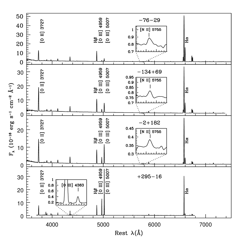
The NGC 628 MMT observations were processed using ISPEC2D (Moustakas & Kennicutt, 2006), a long-slit spectroscopy data reduction package written in IDL, as described in Berg et al. (2011) and Berg et al. (2012). Figure 3 shows a sample of the resulting one-dimensional spectra extracted for H II regions in NGC 628 which had significant [O III] $\lambda$ 4363 or [N II] $\lambda$ 5755 detections. The inset windows display a narrower spectral range to emphasize the auroral line strengths. The NGC 2403 MMT observations were processed following Garnett et al. (1997), with no significant differences.

3 NEBULAR ABUNDANCE ANALYSIS

3.1 Emission Line Measurements

Emission line strengths were measured using standard methods available within IRAF. Specifically, the SPLOT routine was used to analyze the extracted one-dimensional spectra and fit Gaussian profiles to emission lines to determine their integrated fluxes. Special attention was paid to the Balmer lines, which can be located in troughs of significant underlying stellar absorption. In the cases where Balmer absorption was clearly visible, the bluer Balmer lines (H $\delta$ and H $\gamma$ ) were fit simultaneously with multiple components where the absorption was fit by a broad, negative Lorentzian profile and the emission was fit by a narrow, positive Gaussian profile. The negative absorption flux is measure to be roughly consistent for all Balmer lines of a given spectrum, and so for stronger emission lines the absorption component is too weak to measure. This was the case for H $\beta$ and H $\alpha$ in all of our spectra; the absorption component was negligible and not measured. Additional constraints were placed on the faint lines, including the [O III] $\lambda 4363$ and [N II] $\lambda 5755$ auroral lines, such that their FWHMs match the neighboring strong line fits.

Skillman et al. (1994) give a strict accounting of the standard errors ( $\delta L$ ) associated with a given line strength ( $L$ ):

\frac{\delta L}{L}=\frac{\{C_{1}+C_{2}+(n_{o}/\sqrt{n_{s}})S+nAN^{2}+[2.3f(\lambda)\delta C(\mbox{H}\beta)L]^{2}+[0.01L]^{2}+[\delta FL]^{2}\}^{1/2}}{L},

(1)

where $S$ is the sky background in a single row and $n_{o}$ and $n_{s}$ are the number of rows summed over for the object and the sky respectively. Due to the quality of the detectors used the read out noise term ( $nAN^{2}$ ) is negligible compared to the other dominating terms. For weak lines, the uncertainty is dominated by error from the continuum subtraction, meaning that the $C_{2}$ (counts in the continuum) term is the dominating fraction of the $C_{1}$ (total counts in line, continuum, and sky) term. For the lines with flux measurements much stronger than the rms noise of the continuum, (usually the H $\alpha$ lines and often the [O III] $\lambda\lambda$ 4959,5007 doublet) the error is dominated by flux calibration error term ( $[\delta FL]^{2}$ ) and the reddening error term ( $[2.3f(\lambda)\delta C(H\beta)L]^{2}$ ). Thus, in the case of our spectra, the errors of the flux measurements were approximated using

\delta F_{\lambda}\approx\sqrt{{(2\times\sqrt{n_{p}}\times rms)}^{2}+{(0.02\times F_{\lambda})}^{2}},

(2)

where $n_{p}$ is the number of pixels spanning the Gaussian profile fit to the narrow emission lines. The root mean squared ( $rms$ ) noise in the continuum was taken to be the average of the rms on each side of an emission line. Then, the first ( $rms$ ) term determines the approximate uncertainty for the weak lines, and the second ( $F_{\lambda}$ ) term dominates the uncertainty for the strong lines. In the latter case, a minimum uncertainty of 2% was assumed, which is the typical error in fitting flux calibrated points to standard Oke (1990) stars.

11 H II regions in our NGC 628 sample were measured to have [O III] $\lambda$ 4363 and/or [N II] $\lambda$ 5755 line strengths $>4\sigma$ ; three additional objects had auroral line strengths $>3\sigma$ . In NGC 2403, 7 of the H II regions auroral line detections had strengths of $4\sigma$ or greater. Note that the [O III] $\lambda 4363$ line is often difficult to detect due to strong mercury line contamination ( $\lambda 4358$ ) at some observatories, however, NGC 628 has a large enough redshift (z $\sim 0.0022$ ) to clearly distinguish the lines. The redshift for NGC 2403 is lower (z $\sim 0.0004$ ), but this concern is negated by the fact that six of the seven H II regions in our sample also have a temperature measurement from [N II] $\lambda 5755$ . For all of the objects in the present samples, flux line strengths and corresponding errors are listed in Tables 4.5-LABEL:tbl6. We concentrate the rest of our analysis on the objects for which direct electron temperature and chemical abundance determinations can be made.

3.2 Reddening Corrections

The relative intensities of the Balmer lines are nearly independent of both density and temperature, so they can be used to solve for the reddening. The spectra were de-reddened using the reddening law of Cardelli et al. (1989), parametrized by $A_{V}=3.1\ E(B-V)$ , where the extinction, $A_{1}(\lambda)$ was calculated using the York Extinction Solver (McCall, 2004)¹¹1http://www1.cadc-ccda.hia-iha.nrc-cnrc.gc.ca/community/YorkExtinctionSolver/. With these values, the reddening, $E(B-V)$ , can be derived using

\log{\frac{I(H\alpha)}{I(H\beta)}\ }=\log{\frac{F(H\alpha)}{F(H\beta)}\ }+0.4\ E(B-V)\ [A_{1}(H\alpha)-A_{1}(H\beta)],

(3)

where $F$ (H $\alpha)/F$ (H $\beta$ ) is the observed flux ratio and $I$ (H $\alpha)/I$ (H $\beta$ ) is the de-reddened line intensity ratio using case B from Hummer & Storey (1987), assuming an electron temperature calculated from the [O III] line ratio and n ${}_{e}=10^{2}$ cm ${}^{-3}$ . For our NGC 628 sample, the electron temperature covers a range of 6,300 K to 14,100 K in the high ionization zone and from 7,400 K to 13,300 K in the low ionization zone. NGC 2403 exhibits a smaller electron temperature range from 7,700 K to 11,300 K in the high ionization zone and from 8,300 K to 10,900 K in the low ionization zone (see discussion of electron temperatures in Section 3.3). Following Lee & Skillman (2004), the reddening value can be converted to the logarithmic extinction at $H\beta$ as

c(\mbox{H}\beta)=1.43\ E(B-V).

(4)

We evaluate our reddening corrections by using a chi-squared minimization technique in comparing calculated to theoretical values to ensure the best combined solution for the H $\delta$ /H $\beta$ , H $\gamma$ /H $\beta$ , and H $\alpha$ /H $\beta$ ratios (see discussion in Olive & Skillman, 2001). For those cases where underlying absorption was accounted for in measuring the individual emission lines, we fix underlying absorption to be zero in the minimization; otherwise reddening and underlying absorption were solved for simultaneously. For NGC 628 we find a range in $A_{V}$ of 0.13 to 1.56 and a slightly smaller range for NGC 2403 of 0.04 to 1.26. The results are tabulated in Tables 4.5-LABEL:tbl6.

3.3 Electron Temperature and Density Determinations

For H II regions, accurate direct oxygen abundance determinations require reliable electron temperature measurements. This is typically done by observing a temperature sensitive auroral line. We have taken advantage of two such lines: the [O III] $\lambda$ 4363 and [N II] $\lambda$ 5755 auroral lines. To establish a low-uncertainty electron temperature estimate, we define a strong auroral line measurement using a 4 $\sigma$ criterion. In NGC 628, we measured [O III] $\lambda$ 4363 at a strength of 4 $\sigma$ or greater in five H II regions and measured [N II] $\lambda$ 5755 at a strength of 4 $\sigma$ or greater in ten H II regions. Three of these H II regions had both strong [O III] $\lambda$ 4363 and [N II] $\lambda$ 5755 such that we were able to measure 11 total H II regions with direct abundances from at least one strong auroral line. We extend our NGC 628 sample to 14 by including 3 more H II regions that have a 3 $\sigma$ detections of the auroral line.

In NGC 2403, we measured [O III] $\lambda$ 4363 at a strength of 4 $\sigma$ or greater in five H II regions and measured [N II] $\lambda$ 5755 at a strength of 4 $\sigma$ or greater in six H II regions such that all seven H II regions have strong auroral line measurements. For the H II regions in NGC 628 and NGC 2403 with strong auroral lines, we then determined electron temperatures from the associated temperature sensitive “auroral” to “nebular” ratio of collisionally excited lines.

An H II region can be modeled by two separate volumes, one of low ionization and one of high ionization. For the high ionization zone, we used the [O III] I( $\lambda\lambda$ 4959,5007)/I( $\lambda$ 4363) ratio to derive a temperature using the IRAF task TEMDEN. This task computes the electron temperature of the ionized nebular gas within the 5-level atom approximation. The O ${}^{+}$ (low ionization) zone electron temperature can be related to the O ${}^{++}$ (high ionization) zone electron temperature (e.g., Campbell et al., 1986; Pagel et al., 1992). We used the relation between $t_{2}$ ( $T_{e}$ (O ${}^{+}$ )) and $t_{3}$ ( $T_{e}$ (O ${}^{++}$ )) proposed by Pagel et al. (1992), based on the photoionization modeling of Stasińska (1990) to determine the low ionization zone temperature:

t_{e}(\mbox{{O~{}II}})^{-1}=0.5\times[{t_{e}(\mbox{{O~{}III}})}^{-1}+0.8],

(5)

where $t_{e}=T_{e}/10^{4}$ K.

For six of our spectra in NGC 628 and one spectrum in NGC 2403 where a strong [O III] $\lambda$ 4363 was not measured, we were able to determine a temperature using the [N II] I( $\lambda\lambda$ 6548,6584)/I( $\lambda$ 5755) ratio, where we assume $T_{e}$ (N II) = $T_{e}$ (O II). The high ionization zone temperature can then be determined using Equation 5 in reverse. Both the [O III] and [N II] auroral lines were measured in four H II regions in NGC 628 and five H II regions in NGC 2403, allowing us to compare electron temperature estimates for the high ionization zone from two different diagnostics. On average, [O III] predicts a higher electron temperature by 1,100 K in NGC 628 and by 700 K in NGC 2403. While we prioritize the [O III] temperature estimate in this paper, further studies are needed to determine for what cases the [N II] temperature diagnostic is more reliable, and where the differences originate. Note that [O II] $\lambda\lambda 7320,7330$ was measured in multiple H II regions, however, Zurita & Bresolin (2012) have shown that the error in using [O II] is much larger than in using [N II] to derive a temperature for the low ionization zone. In the five H II regions in NGC 628 and four H II regions in NGC 2403 with temperature estimates from both [O II] and [N II], we find that the $T_{e}$ (O II) estimates are 900 K and 600 K larger on average than those from [N II]. This may be due in large part to the fact that the [O II] $\lambda\lambda 7320,7330$ doublet is located in a spectral region containing strong OH airglow emission lines. Additionally, differences in the electron temperature determinations may originate from errors in the standard H II region physics assumed. Peimbert (1967) introduced the temperature inhomogeneity parameter, $t^{2}$ , to be used as a statistical correction to chemical abundances. In order to account for temperature and ionization structures which differ from standard assumptions, Peña-Guerrero et al. (2012) used $t^{2}$ corrections to re-calibrate the strong-line method of Pagel (1985). In a different attempt, Nicholls et al. (2012) suggest that the electrons in a H II region may depart from a Maxwell-Boltzmann equilibrium energy distribution, and instead suggest the adoption of a “ $\kappa$ -distribution”. However, further work is needed to ascertain the most effective solution.

Additionally, we calculate a separate $T_{e}$ (S III) because the S ${}^{++}$ ionization zone lies partially in both the O ${}^{+}$ and the O ${}^{++}$ zones:

t_{e}(\mbox{{S~{}III}})=0.83\times t_{e}(\mbox{{O~{}III}})+0.17.

(6)

The above temperatures are tabulated in Tables LABEL:tbl7-LABEL:tbl9. [S II] $\lambda\lambda$ 6717,6731 was used to determine the electron densities, all of which are consistent with the low density limit. For all abundance calculations we assume $n_{e}=10^{2}$ cm ${}^{-3}$ (which is consistent with the 1 $\sigma$ upper bounds and produces identical results for all lower values of $n_{e}$ ).

3.4 Ionic and Total Abundances

Ionic abundances were calculated with:

{\frac{N(X^{i})}{N(H^{+})}\ }={\frac{I_{\lambda(i)}}{I_{H\beta}}\ }{\frac{j_{H\beta}}{j_{\lambda(i)}}\ }.

(7)

The emissivity coefficients, which are functions of both temperature and density, were determined using the IONIC routine in IRAF with atomic data updated as reported in Bresolin et al. (2009). Note that Nicholls et al. (2013) discuss the the factors involved in obtaining accurate temperatures from collisionally excited lines, showing that significant errors arise when using old collision strength data, and thus using the updated atomic data is crucial. This routine applies the 5-level atom approximation, assuming an electron density of n ${}_{e}=10^{2}$ cm ${}^{-3}$ and the appropriate ionization zone electron temperature.

Total oxygen abundances (O/H) are calculated from the simple sum of O ${}^{+}$ /H ${}^{+}$ and O ${}^{++}$ /H ${}^{+}$ . The other abundance determinations require ionization correction factors (ICF) to account for unobserved ionic species. For nitrogen, we employ the common assumption that N/O = N ${}^{+}$ /O ${}^{+}$ (Peimbert, 1967). This allows us to directly compare our results with other studies in the literature. Nava et al. (2006) have investigated the validity of this assumption. They concluded that it could be improved upon with modern photoionization models, but was valid at the precision of about 10%.

Collisionally excited emission lines of sulfur, neon, and argon were also observed in many of our spectra. For Ne we use a fairly straightforward ICF: ICF(Ne) = (O ${}^{+}$ + O ${}^{++}$ )/O ${}^{++}$ (Crockett et al., 2006). S and Ar present more complicated situations as S ${}^{++}$ and Ar ${}^{++}$ span both the O ${}^{+}$ and the O ${}^{++}$ zones. Thuan et al. (1995) have determined the analytic ICF approximations for both S and Ar using the model calculations of photoionized H II regions by Stasińska (1990). We employ these ICFs from Thuan et al. (1995) to correct for the unobserved S ${}^{+3}$ , Ar ${}^{+2}$ , and Ar ${}^{+4}$ states.

Ionic and total abundances are listed in Tables LABEL:tbl7-LABEL:tbl9. We report direct oxygen abundances for 14 H II regions in NGC 628 (11 of which meet our 4 $\sigma$ criterion) and new direct oxygen abundances for seven NGC 2403 H II regions.

4 THE ABUNDANCE GRADIENTS IN NGC 628 AND NGC 2403

4.1 Oxygen

To analyze the oxygen abundance gradients for NGC 628 and NGC 2403 we have plotted the $3\sigma$ (open circles) and $4\sigma$ (filled symbols) direct abundance detections versus galactocentric radius in Figures 4 and 5 respectively. We determine the most likely linear fits to the data using the FITEXY routine in IDL. This routine uses a least-squares minimization in one-dimension where both independent and dependent variables have associated errors. For the present abundance gradients, the uncertainties in oxygen abundance and galactocentric radius, propagated from the uncertainty of the distance to the galaxy, have been used as weights.

4.1.1 NGC 628

In Figure 4 we plot direct oxygen abundance versus galactocentric radius for NGC 628. The filled points represent all of the targets with direct abundances measured at a strength of 4 $\sigma$ or greater and the open points are three additional H II regions with auroral line detections at a strength of 3 $\sigma$ . Our sample is fairly well dispersed over the range of $R_{g}\sim 2-23$ kpc, containing 10 H II regions within the isophotal radius ( $R_{25}\sim 10.25$ kpc) and four extending beyond $R_{25}$ . As expected from studies of spiral galaxies, the innermost H II regions tend to have higher oxygen abundances and the outermost H II regions have comparatively low oxygen abundances.

The best fit to characterize the gradient of the 11 objects in the current 4 $\sigma$ sample with direct oxygen abundance measurements is given by:

12+\log(\mbox{O/H})=(8.43\pm 0.03)+(-0.017\pm 0.002)\times{R_{g}}\mbox{ (dex/kpc)},

(8)

with a dispersion in log(O/H) of $\sigma$ = 0.10 dex. Additionally, we fit the 3 $\sigma$ sample and found no difference in the resulting fit within the significant digits that we quote here. While the addition of the $3\sigma$ does not alter the fit, we choose to fit only the $4\sigma$ data in order to protect against false detections of the weak auroral lines.

The gas-phase oxygen abundance of NGC 628 has been previously studied using empirical calibrations (e.g., Talent, 1983; McCall et al., 1985; Zaritsky et al., 1994; Ferguson et al., 1998; van Zee et al., 1998; Bresolin et al., 1999; Castellanos et al., 2002; Pilyugin et al., 2004; Moustakas et al., 2010; Gusev et al., 2012; Cedrés et al., 2012), and integral field spectroscopy (e.g., Rosales-Ortega et al., 2011). For comparison, we have plotted the strong-line relationships of Kobulnicky & Kewley (2004) and Pilyugin & Thuan (2005) for NGC 628 as compiled by Moustakas et al. (2010) from literature values. Both methods are based on the metallicity-sensitive $R_{23}$ parameter (Pagel et al., 1979), with an additional excitation parameter that corrects for ionization (referred to as the “P-method”). Using optical spectroscopy of 34 H II regions, Moustakas et al. (2010) found

12+\log(\mbox{O/H})=9.19-0.052\times{R_{g}}\mbox{ (dex/kpc)},

(9)

for the Kobulnicky & Kewley (2004) relationship and

12+\log(\mbox{O/H})=8.43-0.024\times{R_{g}}\mbox{ (dex/kpc)},

(10)

for the Pilyugin & Thuan (2005) relationship, based on 33 H II regions.

Pilyugin et al. (2004) found a significantly steeper gradient in NGC 628 using an earlier version of the P-method (Pilyugin, 2001):

12+\log(\mbox{O/H})=8.68-0.040\times{R_{g}}\mbox{ (dex/kpc)}.

(11)

However, Bresolin et al. (2012) used observations of NGC 1512 and NGC 3621 to show that, of the strong line methods in wide use, the N2 calibration of Pettini & Pagel (2004) best matches the direct abundances. We have applied this method to our observations and plotted the least- squares fit to the results as a dotted-dashed line in Figure 4. Interestingly, this fit lies close to the direct abundances, but has a steeper slope and an approximately 0.2 dex high intercept at the center. Rosales-Ortega et al. (2011) used a variety of methods with integral field spectroscopy to determine the radial oxygen abundance gradient for NGC 628. Using their ff- $T_{e}$ method, they calculated a linear fit of

12+\log(\mbox{O/H})=(8.70\pm 0.01)+(-0.026\pm 0.001)\times{R_{g}}\mbox{ (dex/kpc)}.

(12)

Rosales-Ortega et al. (2011) also examined the gradient using three other strong-line calibrators, finding that the slope of the gradient varies significantly among different calibrators. They conclude that this may be due to the potential for empirical indices based on the [N II] emission lines to overestimate oxygen abundance at high N/O ratios and vice versa (see e.g., Pérez-Montero & Contini, 2009). This is easily seen in our Figure 6 as the Pilyugin & Thuan (2005) and Moustakas et al. (2010) relationships extend to much higher oxygen abundances with increasing N/O .

4.1.2 NGC 2403

The present sample includes three H II regions with reported T(O III) in common with G97: VS 24, VS 44, and VS 9. A comparison of the derived electron temperatures and oxygen abundances shows general, but not perfect agreement. Specifically, for VS 24, G97 derived an O III temperature of 7,600 $\pm$ 400 K and an oxygen abundance of 8.41 $\pm$ 0.09 compared with a temperature of 7,700 $\pm$ 700 K and an oxygen abundance of 8.45 $\pm$ 0.11derived here. For VS 44, G97 derived an O III temperature of 8,300 $\pm$ 400 and an oxygen abundance of 8.49 $\pm$ 0.09 compared with a temperature of 8,700 $\pm$ 200 and an oxygen abundance of 8.40 $\pm$ 0.04 derived here. For VS 9, G97 derived an O III temperature of 11,700 $\pm$ 400 and an oxygen abundance of 8.10 $\pm$ 0.03 compared with a temperature of 11,100 $\pm$ 200 and an oxygen abundance of 8.28 $\pm$ 0.04 derived here. Thus, all of the above measurements agree within 1 $\sigma$ , except for the oxygen abundance of VS 9. As it turns out, G97 did not measure a blue spectrum for VS 9, but, instead, combined the blue spectrum from McCall et al. (1985) with a red spectrum from the MMT. Thus, from the two spectra in common, it appears that the potential non-linearities in the detector are not a concern and that the G97 observations can be compared directly. Given the above, we derive the oxygen abundance gradient both with (1) only the newly obtained observations and (2) from combining the new observations with the previous observations obtained by G97.

In Figure 5 we plot direct oxygen abundance versus galactocentric radius for NGC 2403. Our observations are depicted by solid symbols, the data in common with G97 are given by filled circles and new regions by filled squares. Additional direct observations made by G97 are plotted as open circles. Combining these data, there are 11 points displayed for the inner galaxy extending out to $\sim 10$ kpc. Again we see decreasing oxygen abundance with increasing radius, but with a slightly steeper gradient than that of NGC 628.

The weighted least-squares fit (dotted dahsed line) to the seven new observations (filled symbols) presented here can be expressed as:

12+\log(\mbox{O/H})=(8.46\pm 0.04)+(-0.027\pm 0.008)\times{R_{g}}\mbox{ (dex/kpc)},

(13)

with a dispersion in log(O/H) of $\sigma$ = 0.02 dex. In comparison, the best weighted fit (solid line) to characterize the gradient of the 11 points, both new and old, in NGC 2403 with direct oxygen abundance measurements results in:

12+\log(\mbox{O/H})=(8.48\pm 0.04)+(-0.032\pm 0.007)\times{R_{g}}\mbox{ (dex/kpc)},

(14)

with a dispersion in log(O/H) of $\sigma$ = 0.07 dex. This result is equivalent to the relationship derived for just the new observations, so we carry forward with the addition of the G97 observations to increment our sample.

For NGC 2403, several spectroscopic studies exist where abundances were determined using empirical calibrations (e.g., McCall et al., 1985; Fierro et al., 1986; van Zee et al., 1998; Garnett et al., 1999; Bresolin et al., 1999), as well as a single study using direct abundances (Garnett et al., 1997). The dotted line in Figure 5 is the fit of Pilyugin et al. (2004) using the strong-line P-method (Pilyugin, 2001):

12+\log(\mbox{O/H})=8.52-0.033\times{R_{g}}\mbox{ (dex/kpc)}.

(15)

The dashed line is the fit of Moustakas et al. (2010) using the strong line method from Pilyugin & Thuan (2005):

12+\log({\mbox{O/H}})=8.42-0.032\times{R_{g}}\mbox{ (dex/kpc)}.

(16)

Further, we apply the strong-line N2 calibration (Pettini & Pagel, 2004) recommended by Bresolin et al. (2012) to our data and plot the least-squares fit as a dotted-dashed line in Figure 5. Here the N2 calibration is nearly identical to the P-method of Pilyugin & Thuan (2005). The radial oxygen abundance slope of NGC 2403 is robust, where the fit to direct and strong-line abundance determinations have congruent slopes, but are vertically offset from one another.

4.1.3 Oxygen Abundance in Context

The direct abundance measurements of NGC 628 and NGC 2403 presented here allow comparisons against other spiral galaxies with consistent and reliable derivations. Few previous detailed studies of direct abundances for spiral galaxies exist in the literature, and those that do demonstrate a wide range in abundance gradient slope: $\sim-0.01-0.04$ dex/kpc. For example, Bresolin (2011) found a slope of -0.042 dex/kpc for the oxygen abundance gradient in M33, in contrast to the measurement of -0.012 dex/kpc by Crockett et al. (2006). Other examples include a slope of -0.023 dex/kpc measured for M31 (Bresolin et al., 2012), -0.011 dex/kpc for NGC 4258 (Bresolin, 2011), and -0.020 dex/kpc for M51 (Bresolin et al., 2004). Thus, in comparison, the gradients measured using the direct method for NGC 628 (-0.014 $\pm$ 0.002 dex/kpc) and NGC 2403 (-0.028 $\pm$ 0.007 dex/kpc) are consistent with studies of other non-barred spiral galaxies (e.g., M33, M31, NGC 4258, and M51).

The new direct radial abundance gradients presented here also highlight discrepancies amongst abundance methods when compared to strong-line oxygen abundance calibrations. For NGC 2403, the abundance gradient slope is relatively robust for all abundance calibrations shown in Figure 5. However, the strong-line abundance calibrations from the literature are shifted above and below the direct abundance relationship. For NGC 628, we measure a much shallower direct radial abundance gradient slope relative to a variety of other methods from the literature. In particular, previous studies find higher y-intercepts and thus a significantly higher oxygen abundance predicted for the nucleus of the disk. Among the observations presented in Figure 4, the three direct abundances measured for galactocentric radii less than 5 kpc lie within the vertical scatter of the data, but break from the decreasing abundance trend established at larger radii. These measurements agree with chemical evolution models which predict flatter gradients in the dense inner regions of spirals due to the breakdown of the instantaneous recycling approximation (e.g., Prantzos & Boissier, 2000; Chiappini et al., 2003). The systematically lower direct oxygen abundances measured for NGC 2403 relative to the strong-line P-method gradient of Pilyugin et al. (2004) and the low direct oxygen abundances measured for the inner 5 kpcs of NGC 628 could also be due to temperature fluctuations or gradients. Such temperature inhomogeneities in metal rich H II regions have been shown to cause oxygen abundances to be systematically underestimated by as much as $\sim 0.4$ dex (e.g., Stasińska, 2005; Bresolin, 2007). As discussed in Section 3.3, several methods have recently emerged to correct for these temperature fluctuations (e.g., Peña-Guerrero et al., 2012; Nicholls et al., 2012), but further work is needed to determine if any are universal solutions to the problem.

4.2 Nitrogen

Garnett (1990) found a relatively constant relationship in the N/O ratio versus O/H for low metallicity star-forming galaxies, but with a scatter larger than could be understood in terms of observational uncertainties. He suggested that different delivery times of N and O could explain the relatively large scatter seen in N/O at low metallicities. For example, when a low metallicity galaxy has a burst of star formation, contributions from massive stars will drive O to higher values, while driving N/O values lower. Later, contributions from intermediate mass stars will raise the N/O while keeping O/H constant. Then, if many star-forming galaxies at this oxygen abundance are measured, but are at various times since their burst initiated, a spread in N/O will be seen. At higher metallicities (i.e., 12+log(O/H) $\geq$ 8.0), secondary nitrogen production becomes increasingly significant, causing the average N/O to increase with O/H (Pagel, 1985). We can, therefore, use the radial relationship of N/O in spiral galaxies to determine which nucleosynthetic mechanisms are dominant. We present the absolute and relative nitrogen abundances for NGC 628 and NGC 2403 in Tables LABEL:tbl7-LABEL:tbl9.

4.2.1 NGC 628

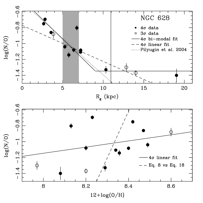
The upper panel of Figure 6 displays the trend of log(N/O) with galactocentric radius in NGC 628. For N/O, the range of values extend from log(N/O) = $-0.69$ at small radii, decreasing outward to $-1.40$ at larger radii. Pilyugin et al. (2004) used a single linear fit to characterize the N/O relationship with galactocentric radii and found a fairly shallow radial gradient (dotted line). Following this approach, we find a much shallower relationship for the 4 $\sigma$ data:

\log(\mbox{N/O})=(-0.49\pm 0.08)+(-0.089\pm 0.011)\times{R_{g}}\ \mbox{ (dex/kpc)},

(17)

with a dispersion in log(N/O) of $\sigma$ = 0.11 dex. This weighted least squares fit to all 11 4 $\sigma$ data points is plotted as a dashed line in Figure 6.

By visual inspection, the data appear to lie in two separate regions. The range from the inner part of the galaxy out to a galactocentric radius of $\approx 10$ kpc, near the luminosity radius ( $R_{25}$ = 10.95 kpc), is fit reasonably well by a steeply declining fit (solid line):

\log(\mbox{N/O})=(-0.45\pm 0.08)+(-0.100\pm 0.013)\times{R_{g}}\ \mbox{ (dex/kpc)},

(18)

with a dispersion in log(N/O) of $\sigma$ = 0.12 dex. This relationship agrees well with the fit found by (Pilyugin et al., 2004), which only sampled the inner galaxy. Beyond $R_{g}$ = 10 kpc, the outer galaxy appears to flatten out in N/O ratio, and so can be fit with a constant value of $\log({\mbox{N/O}})=-1.35$ (solid line), with a dispersion of $\sigma$ = 0.04 dex. The H II regions of NGC 628 measured at distances beyond $R_{25}$ , which have relatively low oxygen abundances (12+log(O/H) $<$ 8.3), have an average N/O ratio that is high relative to the plateau seen for low metallicity dwarf galaxies (e.g., Garnett 1990: log(N/O) = -1.46; van Zee & Haynes 2006: log(N/O) = -1.41; Nava et al. 2006: log(N/O) = -1.43; Berg et al. 2012: log(N/O) = -1.56). However, the average value of $\log({\mbox{N/O}})=-1.35$ measured here for $8.0\lesssim 12+\log({\mbox{O/H}})$ $\lesssim 8.3$ is in agreement with the N/O ratios seen for dwarf galaxies of similar oxygen abundances in Figure 6 of Berg et al. (2012). An additional point worth noting is the scatter in log(N/O) highlighted in the upper panel of Figure 6 for 5 $\lesssim$ $R_{g}\lesssim 7$ . NGC628+185-52 is especially discrepant, deviating by more than 0.2 dex from the linear fit. If this spread is real and not just due to observational uncertainties, it could be indicative of local nitrogen pollution by intermediate mass stars.

The lower panel of Figure 6 allows us to further examine this bi-modal relationship by fitting the N/O ratio over the range in oxygen abundance. The clear trend observed versus radius in the upper panel is not obvious in the plot versus oxygen abundance. If we assume the bi-modal relationship is correct, there are three points with 12+log(O/H) $<$ 8.25 that have N/O values that are located more than 5 $\sigma$ above the average value of the outer disk in the upper panel. It is interesting that the three largest outliers from this plot correspond to the three measurements of oxygen abundance (at the 4 $\sigma$ detection level) below the best fit in Figure 4, including NGC+185-52, which is the highly discrepant point in the upper panel of Figure 6. This could indicate that these regions have oxygen abundances that are underestimated, possibly due to temperature inhomogeneities within the H II region (Peimbert, 1967) or a non Maxwell-Boltzmann electron distribution (Nicholls et al., 2012). If we combine the oxygen abundance radial gradient calculated in Equation 7 with the inner N/O abundance gradient from the upper panel of Figure 6 (Equation 16), the result is the steep dashed line in the lower panel. Based on this relationship, there is a large scatter in N/O abundance for a given oxygen abundance. Instead, the data in the bottom panel of Figure 6 is best fit by a standard linear least-squares fit to the entire data range (solid line):

\log(\mbox{N/O})=-4.25+0.388\times{\mbox{12+log(O/H)}},

(19)

with a dispersion in log(N/O) of $\sigma$ = 0.21 dex. These nitrogen variations offer a different explanation for the divergence of the direct abundance gradient and the strong-line N2 gradient seen for NGC 628 in Figure 4.

Following the method laid out in Zahid & Bresolin (2011), we use a likelihood ratio F-test in order to quantify the significance of the bi-modal model versus the linear model fit. In the case where ${\chi_{1}}^{2}>{\chi_{2}}^{2}$ , the F-statistic is given by

F=\frac{\frac{{\chi_{1}}^{2}-{\chi_{2}}^{2}}{P_{2}-P_{1}}}{\frac{{\chi_{2}}^{2}}{N-P_{2}}},

(20)

where ${\chi_{1}}^{2}$ corresponds to model 1, which is always the simpler model of the two, P is the number of parameters of the fit and N is the number of data points. Under the null hypothesis that model 2 does not give a significantly better fit than model 1, F has an F-distribution characterized by $(P_{2}-P_{1},N-P_{2})$ degrees of freedom. However, if ${\chi_{1}}^{2}$ $<$ ${\chi_{2}}^{2}$ an alternative F-statistic must be used:

F=\frac{{{\chi_{1}}^{2}}/{dof_{1}}}{{{\chi_{2}}^{2}}/{dof_{2}}},

(21)

where the degrees of freedom are given by $dof_{i}=N-P_{i}$ such that F has an F-distribution with $(dof_{1},dof_{2})$ . In the present case, model 1 is a 2-parameter linear fit, with a ${\chi_{1}}^{2}\approx 13.3$ and model 2 is a 5-parameter bi-modal fit (each of the two lines has a parameter for slope and intercept, plus an additional parameter for the location of the break), with a ${\chi_{2}}^{2}\approx 4.7$ . This gives an $F=3.68$ with (3,6) degrees of freedom. We then used the IDL routine MPFTEST (Markwardt, 2009) to determine that the null-hypothesis only has a significance level of 8.2%. This result suggests that model 2 is a significant improvement over model 1 at the 91.8% confidence level, where the break occurs near 12+log(O/H) = 8.3, which roughly corresponds with $R_{g}=R_{25}$ . Thus, we find that while the N/O abundance follows a bi-modal relationship with galactocentric distance, significant variations in either temperature or nitrogen abundance result in a large scatter for a given oxygen abundance.

4.2.2 NGC 2403

The top panel of Figure 7 displays the trend of log(N/O) with galactocentric radius in NGC 2403. The gradient in N/O for NGC 2403 is much shallower at small radii than in NGC 628. Near the center, the measured log(N/O) values only reach $-1.07$ , and then level off at a value of log(N/O) = $-1.42$ past $R_{g}$ = 6 kpc. If we characterize the combined 11 point data set with a single least squares weighted fit (solid line), we find a fit of

\log(\mbox{N/O})=(-1.08\pm 0.02)+(-0.043\pm 0.003)\times{R_{g}}\mbox{ (dex/kpc)},

(22)

with a dispersion in log(N/O) of $\sigma$ = 0.05 dex. Pilyugin et al. (2004) also used a single linear fit to characterize the N/O relationship with galactocentric radii, finding a slightly steeper radial gradient (dotted line):

\log(\mbox{N/O})=-1.040-0.064\times{R_{g}}\mbox{ (dex/kpc)}.

(23)

Unlike the trend seen for N/O in NGC 628, visually the NGC 2403 data do no follow a bi-modal relationship, and an F-test confirms this. However, the luminosity radius for NGC 2403 is $R_{25}=10.1$ kpc, and so the outer optical disk is not sampled by our data set. If the $R_{25}$ of a galaxy is typically where the break in the N/O ratio occurs, then we would not expect to see it in our analysis of NGC 2403, and a declining gradient makes sense with respect to our results for NGC 628. While a general declining trend is observed, note that the vertical spread in the data is relatively small compared to the gradient seen in Figure 6 for NGC 628. At the radial extent of our data, the N/O decline reaches log(N/O) $\sim-1.5$ . Perhaps a plateau in N/O exists near this level farther out in the galaxy (past $R_{25}$ ), similar to the plateau seen for dwarf galaxies (see, e.g., Garnett, 1990; Berg et al., 2012).

In the lower panel of Figure 7 we have plotted 12+log(O/H) vs. log(N/O) for a second look at the N/O relationship. The 4 $\sigma$ data are fit best by a simple least-squares fit (solid line):

\log(\mbox{N/O})=-7.56+0.755\times{\mbox{12+log(O/H)}},

(24)

with a dispersion in log(N/O) of $\sigma$ = 0.10 dex. Again, it is likely that our data did not sample large enough galactocentric radii or low enough metallicities to see the plateau related to primary nitrogen production.

4.2.3 Nitrogen Abundance in Context

If the trends of increasing N/O ratios towards the center of both galaxies are real, it would be indicative of the effects of secondary N production in those regions. Note that Garnett (1990) proposed that much of the scatter in the 12+log(O/H) vs. log(N/O) relationship could be explained by the time delay between producing oxygen in massive stars and secondary nitrogen from intermediate mass stars. Then local nitrogen pollution from intermediate mass stars could provide an explanation for the scatter we see in our data in the inner disks.

In the outer disk, many previous studies note no correlation between 12+log(O/H) and the relative N/O abundance, but do not sample data at radii greater than $R_{25}$ (e.g., Bresolin et al., 2004, 2005; Bresolin, 2011; Zurita & Bresolin, 2012). Barred spiral galaxies are known to show a flattening in their gradient correlated with the strength of their bar (Martin & Roy, 1994). For example, Zahid & Bresolin (2011) measured a break in the strongly barred spiral, NGC 3359, near 12+log(O/H) $\approx 8.3$ , corresponding to radii between $1\cdot R_{25}$ and $1.5\cdot R_{25}$ . Similarly, Kennicutt et al. (2003) found a break near 12+log(O/H) $\approx 8.0$ and $R_{g}=1\cdot R_{25}$ in M101 and Bresolin et al. (2009) showed M83 exhibits a break near $R_{g}=1\cdot R_{25}$ and 12+log(O/H) $\geq 8.3$ . However, a few examples of observed breaks in non-barred spiral galaxies also exist in the literature. Goddard et al. (2011) used a variety of strong-line methods in the mixed spiral galaxy, NGC 4625, to show a break near 12+log(O/H) $>8.3$ at $R_{g}=R_{25}$ and Bresolin et al. (2012) measured a break in the non-barred spiral NGC 3621 near $R_{g}=1\cdot R_{25}$ for oxygen abundances in the range of $8.3<$ 12+log(O/H) $<8.7$ (depending on the abundance method used).

In the present data of NGC 628, and the examples listed above, a pattern is emerging in which N production is transitioning from secondary to primary past $R_{25}$ . Breaks have typically been explained as the result of gas being mixed by radial flows associated with a bar (e.g., Vila-Costas & Edmunds, 1992; Zaritsky et al., 1994; Dutil & Roy, 1999). However, if breaks are observed to be common to all spiral galaxies, then a more general theory will be needed to include non-barred spiral galaxies (for instance, see Bresolin et al. (1999) for discussion of other theories). Furthermore, the break in log(N/O) (near 12+log(O/H) $>8.3$ ) is observed at a much higher oxygen abundance than has been widely observed in dwarf galaxies (see e.g., Garnett, 1990; Izotov & Thuan, 1999; van Zee & Haynes, 2006; Nava et al., 2006; Berg et al., 2012). If further studies confirm this elevated level for turnover, it would have the potential to provide new insights into the production of nitrogen and possible metallicity-dependent yields. Note that Pilyugin (2003) challenged the existence of breaks, showing that artificial breaks can be observed when the strong-line $R_{23}$ method is used to determine abundances. This result further motivates the need for a more significant sample of spiral galaxies with direct abundance gradients and spanning a wide range of Hubble types.

For isolated galaxies there is still no strong consensus on how metals and gas are transported. Possible mechanisms of gas mixing include magnetorotational instabilities (Sellwood & Balbus, 1999), gas outflows and infall (Santillán et al., 2007; Dalcanton, 2007; Zahid et al., 2012), differential rotation (Wada & Norman, 1999), and spiral-bar resonance over-lap (Minchev & Famaey, 2010). Cold mode flows have been measured in several spiral galaxies from H I studies (see e.g., Ryan-Weber et al., 2003; Elson et al., 2010), and are consistent with driving central material outward and mixing into the extended disk, causing higher-than-expected oxygen abundances in the plateau. Salim & Rich (2010) and Lemonias et al. (2011), among others, have argued that cold-mode accretion feeds the ongoing star formation in extended disks, but the low metallicity expected for pristine infalling gas contrasts with the moderately high oxygen abundances measured in the disk. Alternatively, Werk et al. (2011) argue for the hot gas phase mixing scenario proposed by Tassis et al. (2008), an argument nearly identical to those in Kobulnicky & Skillman (1996) and Kobulnicky & Skillman (1997). However, this model assumes that mergers are the dominant source of turbulence, and thus doesn’t answer the question of isolated spiral galaxies. Further, Oppenheimer et al. (2010) suggest a different process of “recycled winds”, where material is driven into the halo by star formation and later reacquired by the galaxy. This idea is supported by observations from Tumlinson et al. (2011) of oxygen rich halos surrounding star-forming galaxies, but which seem to be removed or transformed during the transition to quiescence. As discussed in Bresolin (2011), many questions concerning the mechanisms of galactic disk assembly and evolution remain and will need to be answered using ongoing and future work involving optical spectroscopy of faint H II regions out to large galactocentric radii in spiral galaxies.

4.3 Sulfur, Neon, and Argon

Stellar nucleosynthesis calculations (e.g., Woosley & Weaver, 1995) indicate that $\alpha$ -element and oxygen production occur mainly in massive stars of a small mass range, and thus are expected to trace each other closely. To test this idea in NGC 628 and NGC 2403, we measured the absolute and relative sulfur, neon, and argon abundances, which are tabulated in Tables LABEL:tbl7-LABEL:tbl9.

4.3.1 NGC 628

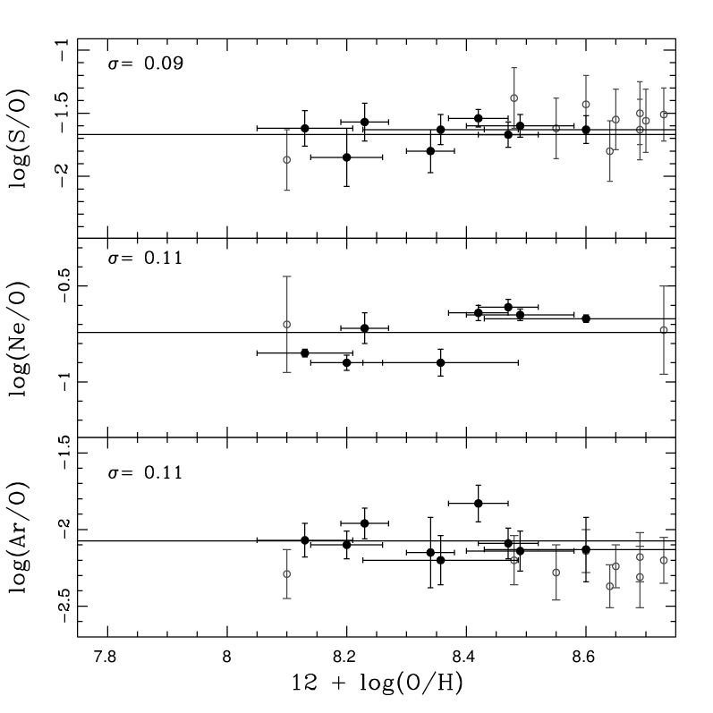
Sulfur, neon, and argon abundances measured for NGC 628 are plotted versus oxygen abundance in Figure 8(a). For each element we have fit the average alpha abundance for the present sample with a solid line and the standard deviation displayed. For comparison, we also determined the error weighted least-squares fit using FITEXY, but found the fits to be no better than the flat relationships. In addition, we plot strong-line abundances from van Zee et al. (1998) as open circles in Figure8(a). We fit the combined data set with a simple least-squares linear relationship, which was found to be nearly constant in all three cases. Even with the addition of the van Zee et al. (1998) data, the scatter around a constant value is small compared to the large range in oxygen abundance sampled. Thus, the $\alpha$ -elements in NGC 628 investigated here can all be described by a constant relationship over oxygen abundance such that the $\alpha$ -elements behave as expected for the nucleosynthetic products of massive stars.

4.3.2 NGC 2403

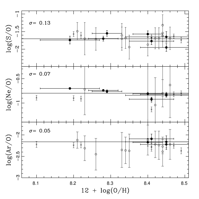
Sulfur, neon, and argon abundances measured for NGC 2403 are plotted versus oxygen abundance in Figure 8(b). Similar to NGC 628, the alpha elements investigated here are fit well by an average alpha abundance for the present sample. The average for each element (solid line) and the standard deviation from these 0-slope fits are illustrated in Figure 8(b). For comparison, we also determined the error weighted least-squares fit using FITEXY and found them to be consistent with the flat relationships plotted. Strong-line abundances are plotted from G97 as crosses and from (van Zee et al., 1998) as open circles, showing that the data from the present sample lies with in the scatter seen around a constant value. These additional data, especially in the case of argon, help to sample a more uniform distribution over the range of oxygen abundance. We fit the combined data set with a simple least-squares linear relationship, which was found to be nearly constant in all three cases. The fact that we are not able to distinguish a trend as more significant than the constant average value indicates that these elements are likely a consequence of massive star nucleosynthesis.

4.3.3 $\alpha$ -Elements in Context

In a comprehensive study of M33, Kwitter & Aller (1981) found that Ne, N, S, and Ar gradients followed that which they derived for oxygen. From stellar nucleosynthesis calculations (e.g., Woosley & Weaver, 1995), oxygen and neon both seem to be produced mainly in stars larger than 10 solar masses, and thus are expected to trace each other closely. Similarly, Henry (1990) finds that Ne/O is constant over a wide range of O/H for planetary nebulae. Thus, the present gradient analysis for NGC 628 and NGC 2403 agree with previous findings that $\alpha$ /O remains constant over the range in oxygen abundance.

In contrast to this viewpoint, Willner & Nelson-Patel (2002) derived a neon gradient that is significantly shallower than the oxygen gradient observed in M33. While sulfur is also traditionally assumed to have a constant S/O ratio (Garnett, 1989), some specific cases, such as the work of Vilchez et al. (1988) on M33, find a slower decline of sulfur than oxygen with radius. Thus, a larger sample of galaxies are needed to determine whether constant $\alpha$ -element abundance gradients are a universal trend amongst spiral galaxies.

The conclusions drawn from Tables LABEL:tbl8-LABEL:tbl9 and Figure 8 support the convention that $\alpha$ -element abundances (S, Ar, and Ne) and O evolve in lockstep for both NGC 628 and NGC 2403. The final adopted fits to the abundance gradients for NGC 628 and NGC 2403 are given in Table 5.

Table 5: Adopted Abundance Gradients for NGC 628 and NGC 2403

y		x	Equation of Correlation	$\sigma$	Portion of Disk
NGC 628
12+log(O/H)	vs.	$R_{g}$	y = (8.43 $\pm$ 0.03) + (-0.017 $\pm 0.002)\times$ x	0.10	Total
log(N/O)	vs.	$R_{g}$	y = (-0.45 $\pm$ 0.08) + (-0.100 $\pm 0.013)\times$ x	0.11	Inner
			y = -1.35	0.04	Outer
log(N/O)	vs.	12+log(O/H)	y = -4.25 + 0.388 $\times$ x	0.21	Total
log(S/O)	vs.	12+log(O/H)	y = -1.67	0.09	Total
log(Ne/O)	vs.	12+log(O/H)	y = -0.74	0.11	Total
log(Ar/O)	vs.	12+log(O/H)	y = -2.07	0.11	Total
NGC 2403
12+log(O/H)	vs.	$R_{g}$	y = (8.48 $\pm$ 0.04) + (-0.032 $\pm 0.007)\times$ x	0.07	Total
log(N/O)	vs.	$R_{g}$	y = (-1.08 $\pm$ 0.02) + (-0.043 $\pm 0.004)\times$ x	0.05	Total
log(N/O)	vs.	12+log(O/H)	y = -7.56 + 0.755 $\times$ x	0.10	Total
log(S/O)	vs.	12+log(O/H)	y = -1.67	0.09	Total
log(Ne/O)	vs.	12+log(O/H)	y = -0.74	0.11	Total
log(Ar/O)	vs.	12+log(O/H)	y = -2.07	0.11	Total

Note. — The adopted best fits to the abundance gradients measured for the 4 $\sigma$ NGC 628 data and the combined sample of present observations plus G97 for NGC 2403.

5 CONCLUSIONS

Spiral galaxies pose a challenge to abundance work, as a single abundance measurement is not sufficient to characterize the entire galaxy. Thus, high quality spectra of many H II regions that enable direct abundances are required to securely measure the oxygen abundance gradient.

We have uniformly determined oxygen abundance metallicities for 14 H II regions in the local spiral galaxy NGC 628 and seven H II regions in NGC 2403. With high-quality spectroscopic observations, we measured the intrinsically faint [O III] $\lambda 4363$ and/or [N II] $\lambda 5755$ auroral lines at a strength of 3 $\sigma$ or greater, and explicitly determine electron temperatures in all 14 H II regions in NGC 628. The seven H II regions in NGC 2403 were chosen to have strong auroral emission lines and, therefore, all have electron temperatures determined at a significance above 4 $\sigma$ .

Our results provide the first ever oxygen abundance gradient derived solely from direct abundance measurements for H II regions in NGC 628. From the $4\sigma$ data we derive an oxygen abundance gradient of 12 + log(O/H) = (8.43 $\pm$ 0.03) + (-0.017 $\pm$ 0.002) $\times{R_{g}}$ (dex/kpc), with a dispersion in log(O/H) of $\sigma$ = 0.10 dex. This is a significantly shallower slope than found by previous empirical abundance studies. As all previous studies of NGC 2403 have relied primarily on strong-line abundances, with only a small number of direct abundances, the seven direct oxygen abundances presented here allow an improved metallicity gradient analysis. The result from these H II regions, which extend from a galactocentric radius of 0.96 to 10.4 kpc, is an oxygen abundance gradient of 12 + log(O/H) = $(8.48\pm 0.04)+(-0.032\pm 0.007)\times{R_{g}}$ (dex/kpc), with a modest dispersion of $\sigma=0.07$ dex.

Additionally, we measure the absolute and relative N, S, Ne, and Ar Abundances. For the N/O ratio we find a negative gradient with increasing galactocentric radius in the inner disks of both NGC 628 and NGC 2403. Further out in the outer disk, this relationship flattens out in NGC 628, where we find a plateau past $R_{g}=R_{25}$ near an oxygen abundance of 12+log(O/H) = 8.3. Similar trends are seen in other spiral galaxies, where the $R_{25}$ radius and oxygen abundances of 12+log(O/H) = 8.3 and greater mark points of transition in nitrogen production. NGC 2403, and other previously studied galaxies, are best fit with a single linear fit. However, in theses cases, the galaxies do not have observations in their extended disks beyond $R_{25}$ and therefore their mechanisms of nitrogen production are not readily comparable to galaxies with observations of greater radial coverage.

As expected for $\alpha$ -process elements, S/O, Ne/O, and Ar/O appear to be constant over a range in oxygen abundance in both NGC 628 and NGC 2403 such that the $\alpha$ -elements and O are produced in lock-step. Since there is a general paucity of abundance data from individual spiral galaxies, more of these accurate H II region datasets are necessary to understand individual galaxy processes and relative trends among galaxies.

We are grateful to the referee for a quick and insightful report which substantially improved the organization and scientific impact of the paper. We are also grateful to Liese van Zee for helpful discussion and the use of her H

\alpha

and R-band imaging. DAB is grateful for support from a Penrose Fellowship, a NASA Space Grant Fellowship, and a Dissertation Fellowship from the University of Minnesota. EDS is grateful for partial support from the University of Minnesota and NSF Grant AST-1109066. Special thanks to Henry Lee for his role helping to prepare the Gemini observations. Observations reported here were obtained at the MMT Observatory, a joint facility of the Smithsonian Institution and the University of Arizona. MMT observations were obtained as part of the University of Minnesota’s guaranteed time on Steward Observatory facilities through membership in the Research Corporation and its support for the Large Binocular Telescope. This work is based, in part, on observations obtained at the Gemini Observatory, which is operated by the Association of Universities for Research in Astronomy, Inc., under a cooperative agreement with the NSF on behalf of the Gemini partnership: the National Science Foundation (United States), the National Research Council (Canada), CONICYT (Chile), the Australian Research Council (Australia), Ministério da Ciência, Tecnologia e Inovação (Brazil) and Ministerio de Ciencia, Tecnología e Innovación Productiva (Argentina). The authors wish to recognize and acknowledge the very significant cultural role and reverence that the summit of Mauna Kea has always had within the indigenous Hawaiian community. We are most fortunate to have the opportunity to conduct observations from this mountain. This research has made use of NASA’s Astrophysics Data System Bibliographic Services and the NASA/IPAC Extragalactic Database (NED), which is operated by the Jet Propulsion Laboratory, California Institute of Technology, under contract with the National Aeronautics and Space Administration. This work was initiated as part of the Spitzer Space Telescope Legacy Science Program and was supported by National Aeronautics and Space Administration (NASA) through contract 1336000 issued by the Jet Propulsion Laboratory (JPL), California Institute of Technology (Caltech) under NASA contract 1407.

References

Aller (1942) Aller, L. H. 1942, ApJ, 95, 52
Berg et al. (2011) Berg, D. A., Skillman, E. D., & Marble, A. R. 2011, ApJ, 738, 2
Berg et al. (2012) Berg, D. A., Skillman, E. D., Marble, A. R., et al. 2012, ApJ, 754, 98
Bresolin (2007) Bresolin, F. 2007, ApJ, 656, 186
Bresolin (2011) —. 2011, ApJ, 730, 129
Bresolin et al. (2004) Bresolin, F., Garnett, D. R., & Kennicutt, Jr., R. C. 2004, ApJ, 615, 228
Bresolin et al. (2009) Bresolin, F., Gieren, W., Kudritzki, R.-P., et al. 2009, ApJ
Bresolin et al. (1999) Bresolin, F., Kennicutt, R. C., J., & Garnett, D. R. 1999, ApJ, 510, 104
Bresolin et al. (2012) Bresolin, F., Kennicutt, R. C., & Ryan-Weber, E. 2012, ApJ, 750, 122
Bresolin et al. (2009) Bresolin, F., Ryan-Weber, E., Kennicutt, R. C., & Goddard, Q. 2009, ApJ
Bresolin et al. (2005) Bresolin, F., Schaerer, D., González Delgado, R. M., & Stasińska, G. 2005, A&A, 441, 981
Campbell et al. (1986) Campbell, A., Terlevich, R., & Melnick, J. 1986, MNRAS, 223, 811
Cardelli et al. (1989) Cardelli, J. A., Clayton, G. C., & Mathis, J. S. 1989, ApJ, 345, 245
Castellanos et al. (2002) Castellanos, M., Díaz, A. I., & Terlevich, E. 2002, MNRAS, 329, 315
Cedrés et al. (2012) Cedrés, B., Cepa, J., Bongiovanni, Á., et al. 2012, A&A, 545, A43
Chiappini et al. (2003) Chiappini, C., Romano, D., & Matteucci, F. 2003, MNRAS, 339, 63
Crockett et al. (2006) Crockett, N. R., Garnett, D. R., Massey, P., & Jacoby, G. 2006, ApJ, 637, 741
Dalcanton (2007) Dalcanton, J. J. 2007, ApJ, 658, 941
Dutil & Roy (1999) Dutil, Y. & Roy, J.-R. 1999, ApJ, 516, 62
Egusa et al. (2009) Egusa, F., Kohno, K., Sofue, Y., Nakanishi, H., & Komugi, S. 2009, ApJ, 697, 1870
Elson et al. (2010) Elson, E. C., de Blok, W. J. G., & Kraan-Korteweg, R. C. 2010, MNRAS, 404, 2061
Engelbracht et al. (2005) Engelbracht, C. W., Gordon, K. D., Rieke, G. H., et al. 2005, ApJ, 628, L29
Engelbracht et al. (2008) Engelbracht, C. W., Rieke, G. H., Gordon, K. D., et al. 2008, ApJ, 678, 804
Esteban et al. (2009) Esteban, C., Bresolin, F., Peimbert, M., et al. 2009, ApJ, 700, 654
Ferguson et al. (1998) Ferguson, A. M. N., Gallagher, J. S., & Wyse, R. F. G. 1998, AJ, 116, 673
Fierro et al. (1986) Fierro, J., Torres-Peimbert, S., & Peimbert, M. 1986, PASP, 98, 1032
Filippenko (1982) Filippenko, A. V. 1982, PASP, 94, 715
Fraternali et al. (2002) Fraternali, F., van Moorsel, G., Sancisi, R., & Oosterloo, T. 2002, AJ, 123, 3124
Garnett (1989) Garnett, D. R. 1989, ApJ, 345, 282
Garnett (1990) Garnett, D. R. 1990, ApJ, 363, 142
Garnett et al. (2004) Garnett, D. R., Edmunds, M. G., Henry, R. B. C., Pagel, B. E. J., & Skillman, E. D. 2004, AJ, 128, 2772
Garnett et al. (1999) Garnett, D. R., Shields, G. A., Peimbert, M., et al. 1999, ApJ, 513, 168
Garnett et al. (1997) Garnett, D. R., Shields, G. A., Skillman, E. D., Sagan, S. P., & Dufour, R. J. 1997, ApJ, 489, 63
Goddard et al. (2011) Goddard, Q. E., Bresolin, F., Kennicutt, R. C., Ryan-Weber, E. V., & Rosales-Ortega, F. F. 2011, MNRAS, 412, 1246
Gusev et al. (2012) Gusev, A. S., Pilyugin, L. S., Sakhibov, F., et al. 2012, MNRAS, 424, 1930
Henry (1990) Henry, R. B. C. 1990, ApJ, 356, 229
Hodge & Kennicutt (1983) Hodge, P. W. & Kennicutt, Jr., R. C. 1983, AJ, 88, 296
Hook et al. (2004) Hook, I., Jørgensen, I., Allington-Smith, J. R., et al. 2004, PASP, 116, 425
Hummer & Storey (1987) Hummer, D. G. & Storey, P. J. 1987, MNRAS, 224, 801
Izotov & Thuan (1999) Izotov, Y. I. & Thuan, T. X. 1999, ApJ, 511, 639
Jacobs et al. (2009) Jacobs, B. A., Rizzi, L., Tully, R. B., et al. 2009, AJ, 138, 332
Jenkins (1987) Jenkins, C. R. 1987, MNRAS, 226, 341
Kendall et al. (2011) Kendall, S., Kennicutt, R. C., & Clarke, C. 2011, MNRAS, 414, 538
Kennicutt et al. (2003) Kennicutt, Jr., R. C., Bresolin, F., & Garnett, D. R. 2003, ApJ, 591, 801
Kobulnicky & Kewley (2004) Kobulnicky, H. A. & Kewley, L. J. 2004, ApJ, 617, 240
Kobulnicky & Skillman (1996) Kobulnicky, H. A. & Skillman, E. D. 1996, ApJ, 471, 211
Kobulnicky & Skillman (1997) —. 1997, ApJ, 489, 636
Kwitter & Aller (1981) Kwitter, K. B. & Aller, L. H. 1981, MNRAS, 195, 939
Lee & Skillman (2004) Lee, H. & Skillman, E. D. 2004, ApJ, 614, 698
Lee et al. (2011) Lee, J. C., de Paz, G., A., K., R. C., J., et al. 2011, ApJS, 192, 6
Lemonias et al. (2011) Lemonias, J. J., Schiminovich, D., Thilker, D., et al. 2011, ApJ, 733, 74
Marble et al. (2010) Marble, A. R., Engelbracht, C. W., van Zee, L., et al. 2010, ApJ, 715, 506
Markwardt (2009) Markwardt, C. B. Astronomical Society of the Pacific Conference Series, Vol. 411, , Astronomical Data Analysis Software and Systems XVIII, ed. D. A. BohlenderD. Durand & P. Dowler, 251
Martin & Roy (1994) Martin, P. & Roy, J.-R. 1994, ApJ, 424, 599
McCall (2004) McCall, M. L. 2004, AJ, 128, 2144
McCall et al. (1985) McCall, M. L., Rybski, P. M., & Shields, G. A. 1985, ApJS, 57, 1
Minchev & Famaey (2010) Minchev, I. & Famaey, B. 2010, ApJ, 722, 112
Moustakas et al. (2010) Moustakas, J., Kennicutt, R. C., J., Tremonti, C. A., et al. 2010, ApJS, 190, 233
Moustakas & Kennicutt (2006) Moustakas, J. & Kennicutt, Jr., R. C. 2006, ApJS, 164, 81
Nava et al. (2006) Nava, A., Casebeer, D., Henry, R. B. C., & Jevremovic, D. 2006, ApJ, 645, 1076
Nicholls et al. (2012) Nicholls, D. C., Dopita, M. A., & Sutherland, R. S. 2012, ApJ, 752, 148
Nicholls et al. (2013) Nicholls, D. C., Dopita, M. A., Sutherland, R. S., Kewley, L. J., & Palay, E. 2013, ApJS, 207, 21
Oke (1990) Oke, J. B. 1990, AJ, 99, 1621
Olive & Skillman (2001) Olive, K. A. & Skillman, E. D. 2001, New A, 6, 119
Oppenheimer et al. (2010) Oppenheimer, B. D., Davé, R., Kereš, D., et al. 2010, MNRAS, 406, 2325
Pagel (1985) Pagel, B. E. J. European Southern Observatory Conference and Workshop Proceedings, Vol. 21, , European Southern Observatory Conference and Workshop Proceedings, ed. I. J. DanzigerF. Matteucci & K. Kjar, 155–170
Pagel & Edmunds (1981) Pagel, B. E. J. & Edmunds, M. G. 1981, ARA&A, 19, 77
Pagel et al. (1979) Pagel, B. E. J., Edmunds, M. G., Blackwell, D. E., Chun, M. S., & Smith, G. 1979, MNRAS, 189, 95
Pagel et al. (1992) Pagel, B. E. J., Simonson, E. A., Terlevich, R. J., & Edmunds, M. G. 1992, MNRAS, 255, 325
Peña-Guerrero et al. (2012) Peña-Guerrero, M. A., Peimbert, A., & Peimbert, M. 2012, ApJ, 756, L14
Peimbert (1967) Peimbert, M. 1967, ApJ, 150, 825
Pérez-Montero & Contini (2009) Pérez-Montero, E. & Contini, T. 2009, MNRAS, 398, 949
Pettini & Pagel (2004) Pettini, M. & Pagel, B. E. J. 2004, MNRAS, 348, L59
Pilyugin (2001) Pilyugin, L. S. 2001, A&A, 369, 594
Pilyugin (2003) —. 2003, A&A, 397, 109
Pilyugin & Thuan (2005) Pilyugin, L. S. & Thuan, T. X. 2005, ApJ, 631, 231
Pilyugin et al. (2004) Pilyugin, L. S., Vílchez, J. M., & Contini, T. 2004, A&A, 425, 849
Prantzos & Boissier (2000) Prantzos, N. & Boissier, S. 2000, MNRAS, 313, 338
Rosales-Ortega et al. (2011) Rosales-Ortega, F. F., Díaz, A. I., Kennicutt, R. C., & Sánchez, S. F. 2011, MNRAS, 415, 2439
Ryan-Weber et al. (2003) Ryan-Weber, E., Webster, R., & Bekki, K. in , Astrophysics and Space Science Library, Vol. 281, The IGM/Galaxy Connection. The Distribution of Baryons at z=0, ed. J. L. RosenbergM. E. Putman, 223
Salim & Rich (2010) Salim, S. & Rich, R. M. 2010, ApJ, 714, L290
Sandstrom et al. (2012) Sandstrom, K. M., Bolatto, A. D., Bot, C., et al. 2012, ApJ, 744, 20
Sandstrom et al. (2013) Sandstrom, K. M. et al. 2013, in preparation
Santillán et al. (2007) Santillán, A., Sánchez-Salcedo, F. J., & Franco, J. 2007, ApJ, 662, L19
Schmidt et al. (1989) Schmidt, G. D., Weymann, R. J., & Foltz, C. B. 1989, PASP, 101, 713
Searle (1971) Searle, L. 1971, ApJ, 168, 327
Sellwood & Balbus (1999) Sellwood, J. A. & Balbus, S. A. 1999, ApJ, 511, 660
Shaver et al. (1983) Shaver, P. A., McGee, R. X., Newton, L. M., Danks, A. C., & Pottasch, S. R. 1983, MNRAS, 204, 53
Shields (1990) Shields, G. A. 1990, ARA&A, 28, 525
Shostak & van der Kruit (1984) Shostak, G. S. & van der Kruit, P. C. 1984, A&A, 132, 20
Sivan et al. (1990) Sivan, J.-P., Maucherat, A. J., Petit, H., & Comte, G. 1990, A&A, 237, 23
Skillman et al. (1994) Skillman, E. D., Televich, R. J., Kennicutt, Jr., R. C., Garnett, D. R., & Terlevich, E. 1994, ApJ, 431, 172
Smith et al. (2005) Smith, J., Armus, L., Dale, D., et al. 2005, Spitzer Proposal, 20518
Smith et al. (2013) Smith, J. et al. 2013, in preparation
Smith et al. (2007) Smith, J. D. T., Draine, B. T., Dale, D. A., et al. 2007, ApJ, 656, 770
Stasińska (1990) Stasińska, G. 1990, A&AS, 83, 501
Stasińska (2005) Stasińska, G. 2005, A&A, 434, 507
Talent (1983) Talent, D. L. 1983, PASP, 95, 986
Tassis et al. (2008) Tassis, K., Kravtsov, A. V., & Gnedin, N. Y. 2008, ApJ, 672, 888
Thuan et al. (1995) Thuan, T. X., Izotov, Y. I., & Lipovetsky, V. A. 1995, ApJ, 445, 108
Tumlinson et al. (2011) Tumlinson, J., Thom, C., Werk, J. K., et al. 2011, Science, 334, 948
Van Dyk et al. (2006) Van Dyk, S. D., Li, W., & Filippenko, A. V. 2006, PASP, 118, 351
van Zee & Haynes (2006) van Zee, L. & Haynes, M. 2006, ApJ, 636, 214
van Zee et al. (1998) van Zee, L., Salzer, J. J., Haynes, M. P., O’Donoghue, A. A., & Balonek, T. J. 1998, AJ, 116, 2805
Véron & Sauvayre (1965) Véron, P. & Sauvayre, A. 1965, Annales d’Astrophysique, 28, 698
Vila-Costas & Edmunds (1992) Vila-Costas, M. B. & Edmunds, M. G. 1992, MNRAS, 259, 121
Vilchez et al. (1988) Vilchez, J. M., Pagel, B. E. J., Diaz, A. I., Terlevich, E., & Edmunds, M. G. 1988, MNRAS, 235, 633
Wada & Norman (1999) Wada, K. & Norman, C. A. 1999, ApJ, 516, L13
Werk et al. (2011) Werk, J. K., Putman, M. E., Meurer, G. R., & Santiago-Figueroa, N. 2011, ApJ, 735, 71
Willner & Nelson-Patel (2002) Willner, S. P. & Nelson-Patel, K. 2002, ApJ, 568, 679
Woosley & Weaver (1995) Woosley, S. E. & Weaver, T. A. 1995, ApJS, 101, 181
Yin et al. (2007) Yin, S. Y., Liang, Y. C., Hammer, F., et al. 2007, A&A, 462, 535
Zahid & Bresolin (2011) Zahid, H. J. & Bresolin, F. 2011, AJ, 141, 192
Zahid et al. (2012) Zahid, H. J., Dima, G. I., Kewley, L. J., Erb, D. K., & Davé, R. 2012, ApJ, 757, 54
Zaritsky et al. (1994) Zaritsky, D., Kennicutt, J., C., R., & Huchra, J. P. 1994, ApJ, 420, 87
Zurita & Bresolin (2012) Zurita, A. & Bresolin, F. 2012, MNRAS, 427, 1463

Table 4.5: Emission-Line Intensities and Equivalent Widths for Gemini Observations of H II regions in NGC 628

	$I(\lambda)/I(\mbox{H}\beta)$
Ion	+9+76	-76-29	-59+84	+82-74	-134+69
[O II] $\lambda$ 3727	1.78 $\pm$ 0.07	1.66 $\pm$ 0.06	2.34 $\pm$ 0.05	1.83 $\pm$ 0.07	2.48 $\pm$ 0.09
H9 $\lambda$ 3835	0.061 $\pm$ 0.005	0.03 $\pm$ 0.01	$\cdots$	$\cdots$	$\cdots$
He I+H8 $\lambda$ 3889	0.23 $\pm$ 0.01	0.22 $\pm$ 0.01	0.32 $\pm$ 0.01	0.12 $\pm$ 0.01	0.17 $\pm$ 0.01
[Ne III]+H7 $\lambda$ 3968	0.16 $\pm$ 0.01	0.13 $\pm$ 0.01	0.15 $\pm$ 0.01	0.11 $\pm$ 0.01	0.14 $\pm$ 0.01
H $\delta$ $\lambda$ 4101	0.28 $\pm$ 0.01	0.27 $\pm$ 0.01	0.26 $\pm$ 0.01	0.27 $\pm$ 0.01	0.27 $\pm$ 0.01
H $\gamma$ $\lambda$ 4340	0.50 $\pm$ 0.02	0.53 $\pm$ 0.01	0.47 $\pm$ 0.01	0.49 $\pm$ 0.01	0.46 $\pm$ 0.01
[O III] $\lambda$ 4363	$\cdots$	$\cdots$	$\cdots$	$\cdots$	$\cdots$
He I $\lambda$ 4471	0.023 $\pm$ 0.003	0.023 $\pm$ 0.002	0.035 $\pm$ 0.03	$\cdots$	0.022 $\pm$ 0.002
H $\beta$ $\lambda$ 4861	1.00 $\pm$ 0.02	1.00 $\pm$ 0.02	1.00 $\pm$ 0.02	1.00 $\pm$ 0.02	1.00 $\pm$ 0.02
[O III] $\lambda$ 4959	0.069 $\pm$ 0.001	0.086 $\pm$ 0.002	0.23 $\pm$ 0.01	0.083 $\pm$ 0.002	0.231 $\pm$ 0.005
[O III] $\lambda$ 5007	0.183 $\pm$ 0.004	0.26 $\pm$ 0.01	0.67 $\pm$ 0.01	0.239 $\pm$ 0.004	0.68 $\pm$ 0.01
N I $\lambda$ 5199	0.013 $\pm$ 0.001	0.020 $\pm$ 0.001	0.013 $\pm$ 0.001	$\cdots$	8.2 $\pm$ 0.8E-4
[N II] $\lambda$ 5755	6.7 $\pm$ 0.5E-3	7.7 $\pm$ 0.5E-3	0.007 $\pm$ 0.001	4.8 $\pm$ 1.6E-3	0.005 $\pm$ 0.001
He I $\lambda$ 5876	0.086 $\pm$ 0.001	0.083 $\pm$ 0.002	0.136 $\pm$ 0.003	0.084 $\pm$ 0.002	0.09 $\pm$ 0.002
[O I] $\lambda$ 6300	0.017 $\pm$ 0.001	0.027 $\pm$ 0.001	0.024 $\pm$ 0.001	0.018 $\pm$ 0.001	0.016 $\pm$ 0.001
[S III] $\lambda$ 6312	3.5 $\pm$ 0.4E-3	0.003 $\pm$ 0.001	0.006 $\pm$ 0.001	0.001 $\pm$ 0.001	0.008 $\pm$ 0.001
[O I] $\lambda$ 6363	6.0 $\pm$ 0.4E-3	0.007 $\pm$ 0.001	0.007 $\pm$ 0.001	0.007 $\pm$ 0.001	0.006 $\pm$ 0.001
[N II] $\lambda$ 6548	0.34 $\pm$ 0.01	0.30 $\pm$ 0.01	0.31 $\pm$ 0.01	0.30 $\pm$ 0.01	0.21 $\pm$ 0.01
H $\alpha$ $\lambda$ 6563	2.98 $\pm$ 0.10	2.99 $\pm$ 0.10	2.97 $\pm$ 0.06	2.94 $\pm$ 0.11	2.85 $\pm$ 0.10
[N II] $\lambda$ 6584	1.02 $\pm$ 0.04	0.93 $\pm$ 0.03	0.92 $\pm$ 0.02	0.88 $\pm$ 0.03	0.64 $\pm$ 0.02
He I $\lambda$ 6678	0.026 $\pm$ 0.001	0.024 $\pm$ 0.001	0.030 $\pm$ 0.001	0.025 $\pm$ 0.001	0.027 $\pm$ 0.001
[S II] $\lambda$ 6717	0.31 $\pm$ 0.01	0.37 $\pm$ 0.01	0.31 $\pm$ 0.01	0.33 $\pm$ 0.01	0.25 $\pm$ 0.01
[S II] $\lambda$ 6731	0.22 $\pm$ 0.01	0.27 $\pm$ 0.01	0.24 $\pm$ 0.01	0.25 $\pm$ 0.01	0.18 $\pm$ 0.01
He I $\lambda$ 7065	0.012 $\pm$ 0.001	0.011 $\pm$ 0.001	0.020 $\pm$ 0.001	0.012 $\pm$ 0.001	0.015 $\pm$ 0.001
[Ar III] $\lambda$ 7136	0.040 $\pm$ 0.002	0.033 $\pm$ 0.001	0.066 $\pm$ 0.001	0.033 $\pm$ 0.001	0.060 $\pm$ 0.003
[C II] $\lambda$ 7236	4.5 $\pm$ 0.3E-3	$\cdots$	$\cdots$	$\cdots$	$\cdots$
He I $\lambda$ 7281	4.4 $\pm$ 0.3E-3	$\cdots$	$\cdots$	0.005 $\pm$ 0.001	3.3 $\pm$ 0.4E-3
[O II] $\lambda$ 7320	10.0 $\pm$ 0.5E-3	$\cdots$	0.018 $\pm$ 0.001	0.013 $\pm$ 0.001	0.018 $\pm$ 0.001
[O II] $\lambda$ 7330	6.9 $\pm$ 0.4E-3	$\cdots$	0.016 $\pm$ 0.001	0.009 $\pm$ 0.001	0.011 $\pm$ 0.001
C(H $\beta$ )	0.71 $\pm$ 0.04	0.55 $\pm$ 0.04	0.72 $\pm$ 0.01	0.58 $\pm$ 0.04	0.30 $\pm$ 0.04
$F$ (H $\beta$ )	73.9 $\pm$ 0.5	88.9 $\pm$ 0.8	52.1 $\pm$ 0.0	57.7 $\pm$ 0.2	75.9 $\pm$ 0.5
EW(H $\beta$ )	226	90.9	143	44.5	67.1
EW(H $\alpha$ )	1340	622	420	361	550.
Ion	-44-159	-2+182	+185-52	-190+80	-90+186
[O II] $\lambda$ 3727	$\cdots$	2.32 $\pm$ 0.09	1.67 $\pm$ 0.06	2.73 $\pm$ 0.10	2.82 $\pm$ 0.06
H10 $\lambda$ 3798	$\cdots$	$\cdots$	$\cdots$	$\cdots$	0.029 $\pm$ 0.003
H9 $\lambda$ 3835	$\cdots$	0.08 $\pm$ 0.01	0.11 $\pm$ 0.004	0.062 $\pm$ 0.003	$\cdots$
[Ne III] $\lambda$ 3868	0.16 $\pm$ 0.01	0.06 $\pm$ 0.01	$\cdots$	0.050 $\pm$ 0.003	0.073 $\pm$ 0.003
He I+H8 $\lambda$ 3889	0.19 $\pm$ 0.01	0.21 $\pm$ 0.01	0.31 $\pm$ 0.01	0.21 $\pm$ 0.01	0.188 $\pm$ 0.003
[Ne III]+H7 $\lambda$ 3968	0.15 $\pm$ 0.01	0.022 $\pm$ 0.005	0.19 $\pm$ 0.01	0.19 $\pm$ 0.01	0.173 $\pm$ 0.001
[S II] $\lambda$ 4068	$\cdots$	$\cdots$	$\cdots$	0.017 $\pm$ 0.002	0.009 $\pm$ 0.001
H $\delta$ $\lambda$ 4101	0.26 $\pm$ 0.01	0.26 $\pm$ 0.01	0.27 $\pm$ 0.01	0.267 $\pm$ 0.007	0.26 $\pm$ 0.01
H $\gamma$ $\lambda$ 4340	0.51 $\pm$ 0.01	0.51 $\pm$ 0.01	0.49 $\pm$ 0.01	0.48 $\pm$ 0.01	0.48 $\pm$ 0.01
[O III] $\lambda$ 4363	0.015 $\pm$ 0.003	$\cdots$	$\cdots$	7.4 $\pm$ 0.8E-3	0.010 $\pm$ 0.001
He I $\lambda$ 4471	0.034 $\pm$ 0.002	0.032 $\pm$ 0.002	0.026 $\pm$ 0.004	0.028 $\pm$ 0.002	0.035 $\pm$ 0.001
[Fe III] $\lambda$ 4658	$\cdots$	$\cdots$	$\cdots$	$\cdots$	0.011 $\pm$ 0.001
He II $\lambda$ 4686	$\cdots$	$\cdots$	$\cdots$	$\cdots$	0.049 $\pm$ 0.001
H $\beta$ $\lambda$ 4861	1.00 $\pm$ 0.02	1.00 $\pm$ 0.02	1.00 $\pm$ 0.02	1.00 $\pm$ 0.02	1.00 $\pm$ 0.02
He I $\lambda$ 4921	$\cdots$	0.009 $\pm$ 0.001	$\cdots$	$\cdots$	8.8 $\pm$ 0.0E-3
[O III] $\lambda$ 4959	0.72 $\pm$ 0.01	0.46 $\pm$ 0.01	0.30 $\pm$ 0.01	0.39 $\pm$ 0.01	0.53 $\pm$ 0.01
[O III] $\lambda$ 5007	2.17 $\pm$ 0.04	1.33 $\pm$ 0.03	0.88 $\pm$ 0.02	1.20 $\pm$ 0.02	1.56 $\pm$ 0.03
N I $\lambda$ 5199	$\cdots$	0.007 $\pm$ 0.001	0.012 $\pm$ 0.001	0.01 $\pm$ 0.01	8.4 $\pm$ 0.3E-3
[Fe III] $\lambda$ 5271	$\cdots$	$\cdots$	$\cdots$	$\cdots$	2.2 $\pm$ 0.4E-3
[Cl III] $\lambda$ 5518	0.005 $\pm$ 0.001	3.9 $\pm$ 0.6E-3	$\cdots$	$\cdots$	$\cdots$
[Cl III] $\lambda$ 5538	$\cdots$	2.4 $\pm$ 0.6E-3	$\cdots$	2.7 $\pm$ 0.4E-3	$\cdots$
[N II] $\lambda$ 5755	0.004 $\pm$ 0.001	0.005 $\pm$ 0.001	0.007 $\pm$ 0.001	5.3 $\pm$ 0.3E-3	5.5 $\pm$ 0.4E-3
He I $\lambda$ 5876	0.126 $\pm$ 0.003	0.111 $\pm$ 0.002	0.106 $\pm$ 0.003	0.103 $\pm$ 0.003	0.131 $\pm$ 0.003
[O I] $\lambda$ 6300	0.021 $\pm$ 0.001	0.016 $\pm$ 0.001	0.022 $\pm$ 0.001	0.032 $\pm$ 0.001	19.5 $\pm$ 0.4E-3
[S III] $\lambda$ 6312	0.009 $\pm$ 0.001	0.009 $\pm$ 0.001	$\cdots$	9.0 $\pm$ 0.3E-3	11.5 $\pm$ 0.4E-3
[O I] $\lambda$ 6363	0.007 $\pm$ 0.001	0.005 $\pm$ 0.001	0.006 $\pm$ 0.001	0.011 $\pm$ 0.001	6.2 $\pm$ 0.4E-3
[N II] $\lambda$ 6548	0.14 $\pm$ 0.01	0.139 $\pm$ 0.005	0.20 $\pm$ 0.01	0.19 $\pm$ 0.01	0.175 $\pm$ 0.004
H $\alpha$ $\lambda$ 6563	2.97 $\pm$ 0.10	2.91 $\pm$ 0.10	2.89 $\pm$ 0.10	2.93 $\pm$ 0.10	2.89 $\pm$ 0.06
[N II] $\lambda$ 6584	0.39 $\pm$ 0.01	0.41 $\pm$ 0.01	0.60 $\pm$ 0.02	0.59 $\pm$ 0.02	0.52 $\pm$ 0.01
He I $\lambda$ 6678	0.038 $\pm$ 0.001	0.033 $\pm$ 0.001	0.032 $\pm$ 0.001	0.031 $\pm$ 0.001	0.031 $\pm$ 0.001
[S II] $\lambda$ 6717	0.22 $\pm$ 0.01	0.19 $\pm$ 0.01	0.29 $\pm$ 0.011	0.34 $\pm$ 0.01	0.235 $\pm$ 0.005
[S II] $\lambda$ 6731	0.16 $\pm$ 0.01	0.135 $\pm$ 0.005	0.20 $\pm$ 0.007	0.25 $\pm$ 0.01	0.171 $\pm$ 0.003
He I $\lambda$ 7065	0.021 $\pm$ 0.001	0.017 $\pm$ 0.001	0.014 $\pm$ 0.001	$\cdots$	19.7 $\pm$ 0.4E-3
[Ar III] $\lambda$ 7136	0.092 $\pm$ 0.004	0.075 $\pm$ 0.003	0.060 $\pm$ 0.003	$\cdots$	0.081 $\pm$ 0.002
He I $\lambda$ 7281	0.005 $\pm$ 0.001	4.6 $\pm$ 0.4E-3	$\cdots$	$\cdots$	$\cdots$
[O II] $\lambda$ 7320	0.017 $\pm$ 0.001	0.018 $\pm$ 0.001	$\cdots$	$\cdots$	$\cdots$
[O II] $\lambda$ 7330	0.014 $\pm$ 0.001	0.014 $\pm$ 0.001	$\cdots$	$\cdots$	$\cdots$
C(H $\beta$ )	0.36 $\pm$ 0.04	0.22 $\pm$ 0.04	0.33 $\pm$ 0.04	0.32 $\pm$ 0.04	0.34 $\pm$ 0.01
$F$ (H $\beta$ )	212 $\pm$ 0	57.9 $\pm$ 0.2	47.3 $\pm$ 0.9	75.7 $\pm$ 0.5	220. $\pm$ 0
EW(H $\beta$ )	71	111	155	174	153
EW(H $\alpha$ )	516	897	1137	1350	1120

Note. — Optical line fluxes for H II regions measured from Gemini NGC 628 spectra using deblended Gaussian fits and multiple component fits when necessary. Fluxes are relative to H $\beta$ = 1.00 and are corrected for reddening. The H $\beta$ flux is given for reference, with units of $10^{-16}$ erg s ${}^{-1}$ cm ${}^{-2}$ . EWs are given in units of Å. Note that uncertainties listed in this table reflect the statistical uncertainties in the flux through the slit only, and do not account for slit losses.