Phase diagram and water-like anomalies in core-softened shoulder-dumbbells system

Abstract

Using molecular dynamics we studied the role of the anisotropy on the phase boundary and on the anomalous behavior of 250 dimeric particles interacting by a core-softened potential. This study led us to an unexpected result: the introduction of a rather small anisotropy, quantified by the distance between the particles inside each dimer, leads to the increase of the size of the regions in the pressure-temperature phase diagram of anomalies when compared to the isotropic monomeric case. However, as the anisotropy increases beyond a threshold the anomalous regions shrinks. We found that this behavior can be understood by decoupling the translational and non-translational kinetic energy components into different translational and non-translational temperatures.

I Introduction

There are liquids in nature that exhibit unexpected thermodynamic or transport properties. Water belongs in this group of anomalous liquids and it is the one with the most puzzling behavior. It expands upon cooling at fixed pressure (density anomaly), diffuses faster upon compression at fixed temperature (diffusion anomaly) and become less ordered upon increasing density at constant temperature (structural anomaly). Despite the complexity of its anomalies, simple molecular water models proved to be able to reproduce many of water unusual properties Ne01 ; Er01 ; An00 .

The origin of water’s anomalies is related to the competition between open low-density and closed high-density structures, which depend on the thermodynamic state of the liquid Kr08 . With the purpose of understanding the nature of these anomalies several models were proposed in which spherically symmetric particles interact with each other by an isotropic potential Sc00 ; Fr01 ; Bu02 ; Bu03 ; Sk04 ; Fr02 ; Ba04 ; Ol05 ; He05 ; He05a ; He70 ; Ja98 ; Wi02 ; Ku04 ; Xu05 ; Ne04 ; Ol06 ; Ol06a ; Ol07 ; Ol08 ; Ol08a ; Ol09 ; Fo08 ; Al09 ; Pr04 ; Gi06 where this competition is described by two preferred interparticle distances.

Among these models, the core-softened shoulder potential proposed by Oliveira et. al.Ol06 ; Ol06a reproduces qualitatively some of the most remarkable water’s anomalies. In particular the regions of density anomaly, diffusion anomaly and structural anomaly obey the same hierarchy as found in real water Ne01 . This potential can represent in an effective and orientation-averaged way the interactions between water clusters characterized by the presence of those two structures (open and closed) discussed above. The open structure is favored by low pressures and the closed structure is favored by high pressures, but only becomes accessible at sufficiently high temperatures.

Even though core-softened potentials have been mainly used for modeling water Ol05 ; Ol06 ; Ol06a ; Ol09 ; Gi06 ; Xu06 ; Ya05 ; Ya06 ; Fr07 , many other materials present the so called water-like anomaly behaviorTh76 ; Ts91 ; Po97 ; An00 ; Sh02 ; Sha06 ; An76 ; Sa03 and, in principle, could be represented by two length potentials. In this sense, it is reasonable to use core-softened potentials as the building blocks of a broader class of materials which we can classify as anomalous fluids. The success of these models raise the question of what properties are not well represented by spherical symmetric potentials.

In a recently study we compared the monomeric model proposed by Oliveira et. al.Ol06 ; Ol06a with a model of dimeric molecules linked as rigid dumbbells, interacting with the same potential. The introduction of anisotropy leads to a much larger region of solid phase in the phase diagram and to the appearance of a liquid crystal phaseOl10 . Later we showed that the size of anomalous regions in the pressure temperature phase diagram is dependent on the value of interparticle separation $\lambda^{*}$ and that the effect of the introduction of a rather small anisotropy due to the dimeric nature of the particle leads to the increase of the size of the regions of anomalies. Nevertheless, the increase of $\lambda^{*}$ shrinks those regions Ne11 .

A possible explanation for this unexpected behavior is that, in conditions of low temperature and pressure, there is a decoupling of translational and rotational degrees of freedom when the interparticle separation is small. Experimental works showed that when approaching the glass transition the translational and rotational dynamics are not equally affected Ha97 ; Ci96 . This behavior was also observed in computer simulations Se12 .

In order to test this hypothesis here we study a dimeric model where each particle in the dimer interacts with the particles in the other dimers through a core-softened potential. We define translational and non-translational temperatures as tools to evaluate the role of translational and non-translational degrees of freedom. Different values of the interparticle separation $\lambda^{*}$ were used and compared.

The remaining of this manuscript goes as follows. In Sec. II the model is introduced and the simulation details are presented. In Sec. III the results are shown and conclusions are exposed in Sec. IV.

II The model

Our model consists of N spherical particles of diameter $\sigma$, linked rigidly in pairs with the distance $\lambda^{*}$ between their centers of mass forming dimers as shown in figure 1. In this way, $\lambda^{*}$ is related to the anisotropy of the dimers. Each particle of the dimer interacts with all particles belonging to other dimers with the intermolecular continuous shoulder potential Ol06 ; Ol10 given by

$$U^{*}(r)=\frac{U(r)}{\epsilon}=4\left[\left(\frac{\sigma}{r}\right)^{12}-\left(\frac{\sigma}{r}\right)^{6}\right]+a\exp\left[-\frac{1}{c^{2}}\left(\frac{r-r_{0}}{\sigma}\right)^{2}\right]\;.$$ (1)

Depending on the choice of the values of $a$, $r_{0}$ and $c$ a whole family of potentials can be built, which shapes ranging from a deep double wellsNe04 ; Th76 to a repulsive shoulderJa98 . In our simulations we used $a=5$, $r_{0}/\sigma=0.7$, $c=1$ and $\lambda/\sigma=0.10,0.20,0.50$ and $0.70$.

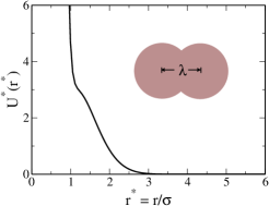
Figure 1: Effective potential versus distance in reduced units.

We performed molecular dynamics simulations in the canonical ensemble using $N=500$ particles (250 dimers) in a cubic box of volume $v$ with periodic boundary conditions in three directions, interacting with the intermolecular potential described above. The cutoff radius was set to $5.5\sigma$ length units. Pressure, temperature, density and diffusion are calculated in dimensionless units

$$T^{*}\equiv\frac{k_{B}T}{\epsilon}$$

$$\rho^{*}\equiv\rho\sigma^{3}$$

$$P^{*}\equiv\frac{P\sigma^{3}}{\epsilon}$$

$$D^{*}\equiv\frac{D(m/\epsilon)^{1/2}}{\sigma}$$

$$t^{*}\equiv t\left(\frac{\varepsilon}{m\sigma^{2}}\right)^{1/2}$$

$$\lambda^{*}\equiv\frac{\lambda}{\sigma}$$

Thermodynamic and dynamic properties were calculated over 700 000 steps after previous 300 000 equilibration steps. The time step was 0.001 in reduced units, the time constant of the Berendsen thermostat Be84 was 0.1 in reduced units. The internal bonds between the particles in each dimer remain fixed using the algorithm SHAKE Ry77 with a tolerance of $10^{-12}$ and maximum of 100 interactions for each bond.

The structure of the system was characterized using the intermolecular radial distribution function, $g(r)$ (RDF), which does not take into account the correlation between particles belonging to the same dimers. The diffusion coefficient was calculated using the slope of the least square fit to the linear part of the mean square displacement, $<r^{2}(t)>$ (MSD), averaged over different time origins. Both the $g(r)$ and $<r^{2}(t)>$ where computed relative to the center of mass of a dimer. The phase boundary between the solid and fluid phases was mapped by the analysis of the change of the pattern of mean square displacement and radial distribution function Ne11 .

In a previous work Ol10 we showed that, depending on the chosen temperature and density, the system could be in a fluid phase metastable with respect to the solid phase. In order to locate the phase boundary two sets of simulations were carried out, one beginning with molecules in a ordered crystal structure and other beginning with molecules in a random, liquid, starting structure obtained from previous equilibrium simulations.

We define the structural anomaly region as the region where the translational order parameter $t$ given by

$$t=\int_{0}^{\xi_{c}}|g(\xi)-1|d\xi$$ (2)

decreases upon increasing density. Here $\xi\equiv r\rho^{1/3}$ is the distance $r$ scaled in units of mean interparticle separation, computed by the center of mass of the dimers, $\xi_{c}$ is the cutoff distance set to half of simulation box times $\rho^{1/3}$ Ol06a and $g(\xi)$ is the radial distribution function as a function of the scaled distance $\xi$ from a reference particle. For an ideal gas $g=1$ and $t=0$. In the crystal phase $g\neq 1$ over long distances and $t$ is large.

The dynamic of the system was analyzed through the mean square displacement (which allows to calculate the diffusion coefficient) and the velocity and orientational autocorrelation function. The velocity autocorrelation function is calculated taking the average for all dimers and initial times through the expression

$$v_{acf}(t)=\langle\mathbf{v}_{i}(t_{0})\cdot\mathbf{v}_{i}(t_{0}+t)\rangle$$ (3)

where $\vec{v}_{i}(t_{0})$ is the initial velocity vector for the dimer $i$ and $\vec{v}_{i}(t_{0}+t)$ is the velocity vector for the same dimer at a later time $t_{0}+t$. The orientational autocorrelation function is defined by

$$O^{l}_{acf}(t)=\langle P_{l}(cos\theta_{i})\rangle$$ (4)

where $P_{l}$ is the Legendre polynomials of order $l$ and $\theta_{i}$ is the reorientation angle of the intra-dimer vector during the time interval $\Delta t$.

III Results

III.1 P-T phase diagram for different values of $\lambda^{*}$

In previous work Ol10 , we studied a system of 250 dimer, interacting through the interparticle potential (1) with $\lambda^{*}=0.20$ in a broad range of densities and temperatures. The pressure, radial distribution function, mean square displacement and diffusion coefficient were calculated for all state points, yielding a complete description of the regions of structural, density and diffusion anomalies.

The comparison between the monomeric case and the dimeric case with $\lambda^{*}=0.20$ showed in the pressure vs temperature phase diagram that the anisotropy due the dumbbells leads to larger range of pressures and temperatures occupied by anomalous regions and by the solid phase Ol10 .

This result raises questions about the influence of anisotropy on the phase and anomalous behavior. In principle one could expect that by increasing the anisotropy by enlarging $\lambda^{*}$ the solid-fluid phase boundary, the TMD line and the diffusion anomalous region would move to higher temperatures. In order to check this assumption we carried out a detailed set of simulations of rigid dumbbells interacting with the potential described above with $\lambda^{*}=0.50$ Ne11 . Figure 2 shows the complete pressure-temperature phase diagram for this system and for the system with $\lambda^{*}=0.20$. This figure shows that the boundaries of the anomalous regions depend clearly on $\lambda^{*}$. The solid-fluid phase boundary and the TMD are shifted towards lower temperatures and slightly higher pressures with the increase of $\lambda^{*}$. The high-temperature limit of the boundary of the region of diffusion anomalies also becomes shifted towards lower temperatures, whereas the lower-temperature part of this region becomes broader. The structurally anomalous region shrinks with increasing $\lambda^{*}$.

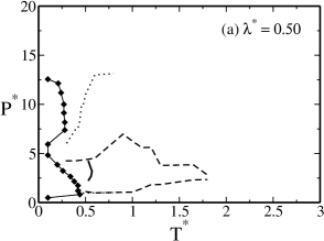
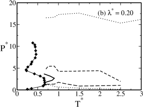
Figure 2: Pressure temperature phase diagram for (a)$\lambda^{*}=0.50$ and (b)$\lambda^{*}=0.20$ interacting through the potential illustrated in Fig. 1. The bold line with diamonds represent the boundary between the fluid and solid phases and the bold, dashed and dotted lines represent the TMD, the region of diffusion anomaly and the region of structural anomaly respectively.

In order to confirm the influence of $\lambda^{*}$ on the phase diagram and regions of anomalous behavior, several simulations restricted to a small region in the phase diagram were carried out. These simulation explored the densities between $\rho^{*}=0.10$ and $\rho^{*}=0.30$ and the temperatures betwenn $T^{*}=0.10$ and $T^{*}=0.80$ for $\lambda^{*}=0.10,0.20,0.50$ and $0.70$. Figure 3 the solid-fluid phase boundary in the pressure temperature phase diagram for $\lambda^{*}=0.10,0.20,0.50$ and $0.70$. The figure shows that the increase of the interparticle separation shifts the solid-fluid phase boundary to lower temperatures.

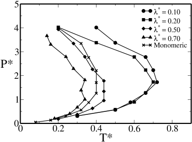
Figure 3: Solid-fluid phase boundary for different values of interparticle separation $\lambda^{*}$ and for monomeric caseOl06 ; Ol06a .

Comparing the results of the simulations corresponding to the several values of $\lambda^{*}$ with the results of the monomeric shoulder-potential simulationsOl06 ; Ol06a , a non-monotonic behavior is observed instead of having the monomeric case as the limit of $\lambda^{*}\rightarrow 0$. In order to check why as $\lambda^{*}\rightarrow 0$, the system does not converge to the monotonic case, the orientational degrees of freedom are analyzed.

Autocorrelation functions are very powerful tools to describe dynamics therefore the analysis of these curves can give us an idea why the solid-fluid phase boundary is contracting with the increase of $\lambda^{*}$. Fig. 4 shows velocity autocorrelation functions, $v_{acf}(t)$, orientational autocorrelation function, $O_{acf}(t)$, and mean square displacement, $<r^{2}(t)>$, for simulations with different values of $\lambda^{*}$ subject to the same conditions of density and temperature.

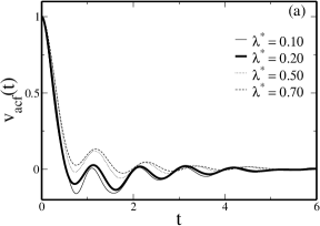
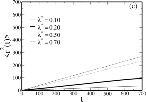
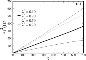
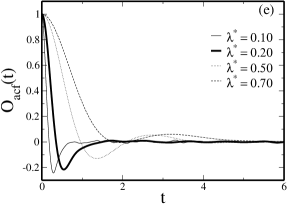
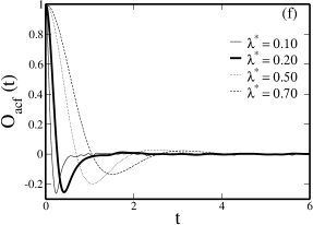
Figure 4: Velocity autocorrelation function, $v_{acf}(t)$ for (a)$T^{*}=0,30$ and (b)$T^{*}=0,50$, mean square displacement, $<r^{2}(t)>$ for (c)$T^{*}=0,30$ and (d)$T^{*}=0,50$, and orientational autocorrelation function, $O_{acf}(t)$ for (e)$T^{*}=0,30$ and (f)$T^{*}=0,50$. All the graphs are for $\rho^{*}=0.30$.

The velocity autocorrelation function $v_{acf}$ versus time, illustrated in Fig. 4, shows that for all the values of $\lambda^{*}$ the curves present a fast decay, however, only the curves for small interparticle separation $\lambda^{*}$ cross the zero axis at short time, i.e, only the velocity vectors for small $\lambda^{*}$’s change signal. This result indicate that the less anisotropic particles (small $\lambda^{*}$) ”feel”the cage of neighbors molecules more strongly than the more anisotropic particles. With the increase of the temperature this effect is weakened, consequently the behavior of $v_{acf}$ for $\lambda^{*}=0.10$ and $T^{*}=0.50$ is similar to the behavior of $\lambda^{*}=0.20$ and $T^{*}=0.30$. Therefore the increase of the temperature compensates the decrease of the $\lambda^{*}$ value.

The slope of mean square displacement, illustrated in Fig. 4, is related with the translational diffusion. For density $\rho^{*}=0.30$ and $T^{*}=0.30$, the larger the interparticle separation, $\lambda^{*}$, the larger the translational diffusion of the system would be. With the increase of the temperature all systems become more diffusive, however, the largest change occurs for the small values of $\lambda^{*}$ . At a fixed temperature thehe relative difference between the curves given by:

$$\frac{<r^{2}(t=700,\lambda^{*}=0.70,T^{*}=0.30)>}{<r^{2}(t=700,\lambda^{*}=0.10,T^{*}=0.30)>}=7.77$$

$$\frac{<r^{2}(t=700,\lambda^{*}=0.70,T^{*}=0.50)>}{<r^{2}(t=700,\lambda^{*}=0.10,T^{*}=0.50)>}=3.47$$

The orientational autocorrelation function, $O_{act}$, is also shown in the Fig. 4. The less anisotropic systems for $\rho^{*}=0.30$ and $T^{*}=0.30$ have a $O_{act}$ that decays quickly to zero.This result indicates that, for these systems, the time needed to perform a $90^{o}$ rotation is very small, i.e., systems with small interparticle separation rotate much easier then systems with larger $\lambda^{*}$ values. For all the interparticle separations, $\lambda^{*}$, the orientational mobility is facilitated by the increase of the temperature. It is noteworthy that the differences in $O_{act}$ (Fig. 4(e) e Fig. 4(f)) are much stranger that the difference in $v_{acf}$ (Fig. 4(a) e Fig. 4(b)).

The analysis of the behavior of $<r^{2}(t)>$, $v_{acf}$ and $O_{act}$ for several values of $\lambda^{*}$, $\rho^{*}$ and $T^{*}$ leads to the conclusion that the more anisotropic systems diffuse faster than the less anisotropic particles but rotate slower than systems with low anisotropy (small $\lambda^{*}$). Based on these observation we raised the hypothesis that the shrinking of the region of solid phase is related to a decoupling between translational and non-translational motions.

In order to test our hypothesis we defined a translational temperature and a non-translational temperature as tools to evaluate the role of translational and non-translational degrees of freedom.

III.2 Translational and non-translational temperatures

In our dimeric system simulations, as well as in our monomeric simulations Ol06 ; Ol06a , Berendsen thermostat is used to maintain the temperature fixed. In this thermostat the temperature of the system is defined as the kinetic energy of the system divided by the number of degrees of freedom. When we are dealing with monomeric systems the temperature has only the contribution of the translational kinetic energy but when dealing with the dimeric systems, the temperature has the translational plus the rotational (and eventually vibrational) kinetic energy contributions. In other words, due to its rotational or vibrational kinetic energy, a dimeric particle rotating or vibrating around a single point has a non zero temperature, even though its center of mass remains still. Since the dimeric system is composed by hard-linked particles the internal vibration is excluded, remaining only the rotational and hindered rotational (libration) motions.

In order to test the effect in the pressure versus temperature phase diagram of the decoupling of the temperature we calculated separately the contributions of translational movement, which we associate with a translational temperature, and non-translational movement, associated with a non-translational temperature. Each degree of freedom contribute with $k_{B}T/2$ to the kinetic energy.

The contributions of translational movement were obtained calculating the kinetic energy of the center of mass of the dimeric particles, $K_{trans}$. Thus if the dimeric particle is rotating around a single point the translational contribution will be zero. Since there are $N/2$ dimers, the translational temperature is defined by

$$K_{trans}=3\frac{N}{2}\frac{k_{B}T_{trans}}{2}$$ (5)

Non-translational temperature was also defined using the equipartition theorem. The internal energy of our full system is given by

$$K=f\frac{k_{B}T}{2}=5\frac{N}{2}\frac{k_{B}T}{2}$$ (6)

where $f$ is the number of degree of freedom of the system. $f$ is equal to the number of dimers $N/2$ times the number of degrees os freedom of each dimer. One degree of freedom of the dimer is lost due the internal bonds between the particles that belong to the dimer. The non-translational contributions of internal energy is

$$K_{ntrans}=\frac{N}{2}k_{B}T_{ntrans}$$ (7)

where $T_{ntrans}$ is the non-translational temperature. Using this equation and considering $K=K_{trans}+K_{ntrans}$ we can write an expression for the non-translational temperature

$$T^{*}_{ntrans}=\frac{5}{2}T^{*}-\frac{3}{2}T^{*}_{trans}$$ (8)

Using this approach we analyzed the influence of interparticle separation on the decoupling between translational and non-translational motion. Figure 5 shows $T^{*}_{trans}$ vs $T^{*}_{ntrans}$ comparing different values of $\lambda^{*}$ for several densities. For small $\lambda^{*}$, a linear behavior $T^{*}_{trans}=a^{(\rho)}T^{*}_{ntrans}$ is observed but only for a certain interval of densities. As the density increases $a(\rho)\rightarrow 1$. According to the definitions described above, this means that, for small interparticle separation, the system can easily perform a non-translational motion without performing a translational one. As the density and the total temperature increase the motions of the system become more correlated. For higher values of $\lambda^{*}$ the decoupling is not observed. For all densities $T^{*}_{trans}=T^{*}_{ntrans}$. In these cases the non-translational motion is strongly dependent (coupled) on translational motion.

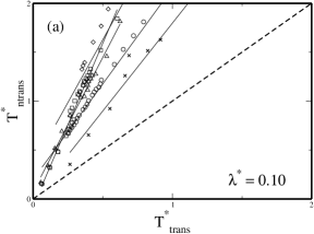
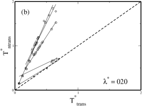
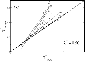
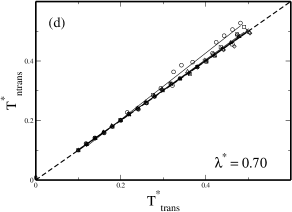
Figure 5: Translational temperature vs non-translational temperature for $(a)\lambda^{*}=0.10,(b)\lambda^{*}=0.20,(c)\lambda^{*}=0.50$ and $(d)\lambda^{*}=0.70$. In each case results with $\rho^{*}=0.10,0.14,0.20,0.26$ and $0.30$ are shown.

For a deeper analysis of the effects linked to the different degrees of freedom we rescaled the pressure temperature phase diagram using the translational and non-translational temperature. Figure 6(a) shows that the rescaled solid-fluid phase boundary with respect the translational temperature moves backwards in such a way that all the curves get closer, almost collapsing. However, when we rescale the phase boundary with non-translational function we could observe the opposite behavior. The curves moves forth and they separate further from each other.

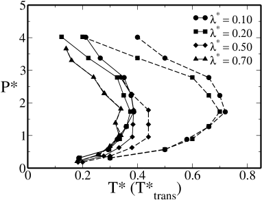
Figure 6: Solid-fluid phase boundary for different $\lambda^{*}$. The solid lines represent the solid-fluid phase boundary rescaled with translational temperature, the dashed lines represent the original phase boundary.

The behavior of the solid-fluid boundary, as well as the anomalous region in the pressure-temperature phase diagram are, in fact, sensitive to translational temperature. Indeed, in systems where molecules are able to perform non-translational movements without perform translational ones, as in the case of small $\lambda^{*}$, the dimers interacts with the other dimers in such a way that their center of mass stay ordered in a solid lattice. Thus, the translational temperature acts like the true effective temperature.

Systems with smaller interparticle separation $\lambda^{*}$ present a larger difference between the translational temperature and the formal temperature than systems with larger $\lambda^{*}$, due to the decoupling of translational and non-translational degrees of freedom. This difference is responsable for the apparent non-monotonic behavior of the region of solid phase.

In order to highlight the effects due the translational degrees of freedom, figure 7 shows the solid-fluid phase boundary rescaled using the translational temperature for several $\lambda^{*}$ and the solid-fuid phase boundary for the monomeric system.

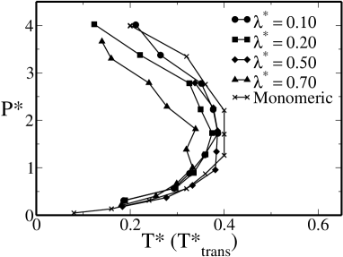
Figure 7: Solid-fluid phase boundary for different $\lambda^{*}$ reescaled with translational temperature and Solid-fluid phase boundary for the monomeric system.

We can observe that, taking in to account only translational movements, the introduction of an anisotropy makes the region of solid phase lightly move backwards in temperature. We also observe that $\lambda^{*}=0.10,0.20$ and $0.50$ almost collapsed in one region indicating the solid-fluid phase boundary depends effectivelly on the translational part of the temperature. Therefore the unexpected non-monotonic behavior is due the non-translational motion as we predicted before. Small dimeric particles can easily perform a non-translational motion and therefore, despite having a formal high temperature, behave as a solid, due to their low translational temperature..

The phase boundary for $\lambda^{*}=0.70$ does not collapsed like the other ones. The reason behind this observation remains still an open question.

Despite of $\lambda^{*}=0.70$ we can affirm that the non-monatomic behavior is essentially due the difference between translational temperature and the formal temperature.

IV Conclusion

We performed molecular dynamics with rigid dimers in which each monomer interacts with monomers from other dimers through a core-softened shoulder potential in order to study the influence of anisotropy in anomalous regions and solid-fluid phase boundary. We carried out simulations for interparticle separation $\lambda^{*}=0.10,0.20,0.50$ and $0.70$ and we observed an unexpected non-monotonic behavior where the solid phase shrinks with increase of $\lambda^{*}$.

Through the analysis of velocity and orientational autocorrelation functions and the mean square displacement we formulated a hypothesis that decoupling between translational and non-translational motion would be responsible for the shrinking of the region of solid phase in the phase diagram.

In order to test these hypothesis we defined the translational and non-translational temperatures obteined from the kinetic energy as tools to evaluate the role of translational and non-translational degrees of freedom. We obtained that for simulations with small values of $\lambda^{*}$ the non-translational temperature is much higher than the translational one. For larger values of $\lambda^{*}$ the temperatures are correlated independently of density and temperature. These results are consistent with the non-monotonic behavior observed.

We rescaled the pressure temperature phase diagram in order to obtain a pressure vs translational temperature phase diagram and observed the behavior of solid phase. We argue that translational temperature is the true effective temperature and that the non-monotonic behavior of solid-fluid phase boundary is due the difference between translational temperature and the formal temperature. We observed that the introduction of anisotropy leads to a smaller region of solid phase when compared with monomeric system and that the solid-fluid phase boundary for $\lambda^{*}=0.10,0.20$ and $0.50$ collapsed on one region of phase diagram.

Despite of that we still have open questions since the phase boundary for $\lambda^{*}=0.70$ did not collapsed like the others. The reason behind that could be related to the size of the dimer. Nevertheless we succeeded to explain most part of the reasons that led to the non-monotonic behavior of solid-fluid boundary which lead us one step forward in the understanding of more complex systems.

References

- (1) P. A. Netz, F. W. Starr, H. E. Stanley and M. C. Barbosa,J. Chem. Phys.115, 344 (2001).
- (2) J. R. Errington and P.D. Debenedetti, Nature (London) 409 318 (2001).
- (3) C. A. Angell, R. D. Bressel, M. Hemmatti, E. J. Sare and J. C. Tucker, Phys. Chem. Chem. Phys. 2 1559 (2000).
- (4) W. P. Krekelberg, J. Mittal, V. Ganesan and T. M. Truskett, Phys. Rev. E 77 041201 (2008).
- (5) A. Scala, M. R. Sadr-Lahijany, N. Giovambattista, S. V. Buldyrev, and H. E. Stanley, J. Stat. Phys. 97 100 (2000).
- (6) G. Franzese, Malescio, A. Skibinsky, S. V. Buldyrev and H. E. Stanley, Nature (London) 409 692 (2001).
- (7) S. V. Buldyrev, G. Franzese, N. Giovambattista, G. Malescio, M. R. Sadr-Lahijany, A. Scala, A. Skibinsky, and H. E. Stanley, Physica A 304 23 (2002).
- (8) S. V. Buldyrev and H. E. Stanley, Physica A 330 124 (2003).
- (9) A. Skibinsky, S. V. Buldyrev, G. Franzese, G. Malescio and H. E. Stanley, Phys. Rev. E 69 061206 (2005.
- (10) G. Franzese, G. Malescio, A. Skibinsky, S. V. Buldyrev and H. E. Stanley, Phys. Rev. E 66 051206 (2002).
- (11) A. Balladares and M. C. Barbosa, J. Phys.: Cond. Matter 16 8811 (2004).
- (12) A. B. de Oliveira and M. C. Barbosa, J. Phys.: Cond. Matter 17 399 (2005).
- (13) V. B. Henriques and M. C. Barbosa, Phys. Rev. E 71 031504 (2005).
- (14) V. B. Henriques, N. Guissoni, M. A. Barbosa, M. Thielo and M. C. Barbosa, Mol. Phys. 103 3001 (2005).
- (15) P. C. Hemmer and G. Stell, Phys. Rev. Lett. 24 1284 (1970).
- (16) E. A. Jagla, Phys. Rev. E 58 1478 (1998).
- (17) N. B. Wilding and J. E. Magee, Phys. Rev. E 66 031509 (2002).
- (18) R. Kurita and H. Tanaka, Science 306 845 (2004).
- (19) L. Xu, P. Kumar, S. V. Buldyrev, S. -H. Chen, P. Poole, F. Sciortino and H. E. Stanley, Proc. Natl. Acad. Sci. U.S.A. 102 16558 (2005).
- (20) P.A. Netz, J. F. Raymundi, A. S. Camera and M. C. Barbosa, Physica A 342 48 (2004).
- (21) A. B. de Oliveira, P. A. Netz, T. Colla and M. C. Barbosa, J. Chem. Phys. 124 084505 (2006).
- (22) A. B. de Oliveira, P. A. Netz, T. Colla and M. C. Barbosa, J. Chem. Phys. 125 124503 (2006).
- (23) A. B. de Oliveira, M. C. Barbosa and P. A. Netz, Physica A 386 744 (2007).
- (24) A. B. de Oliveira, P. A. Netz, and M. C. Barbosa, European Physics Journal B 64 481 (2008).
- (25) A. B. de Oliveira, G. Franzese, P. A. Netz, and M. C. Barbosa, J. Chem. Phys. 128 064901 (2008).
- (26) A. B. de Oliveira, P. A. Netz and M. C. Barbosa, Euro. Phys. Lett 85 36001 (2009).
- (27) Yu. D.Fomin, N. V.Gribova, V. N. Ryzhoy, S.M. Stishov and D. Frenkel, J. Chem. Phys. 129 064512 (2008).
- (28) N. G. Almarza, J. A. Capitan, J. A. Cuesta and E. Lomba, J. Chem. Phys. 131 124506 (2009).
- (29) M. Pretti and C. Buzano, J. Chem. Phys. 121 11856 (2004).
- (30) H. M. Gibson and N. B. Wilding, Phys. Rev. E 73 061507 (2006).
- (31) L. Xu, S. Buldyrev, C. A. Angell and H. E. Stanley, Phys. Rev. E 74 031108 (2006).
- (32) Z. Yan, S. V. Buldyrev, N. Giovambattista and H. E. Stanley, Phys. Rev. Lett. 95 130604 (2005).
- (33) Z. Yan, S. V. Buldyrev, N. Giovambattista, P. G. Debenedetti and H. E. Stanley, Phys. Rev. E 73 051204 (2006).
- (34) G. Franzese, J. Mol. Liq. 136 267 (2007).
- (35) H. Thurn and J. Ruska, J. Non-Cryst. Solids 22, 331 (1976).
- (36) T .Tsuchiya, J. Phys. Soc. Jpn. 60, 227 (1991).
- (37) P. H. Poole, M. Hemmati and C. A. Angell, Phys. Rev. Lett. 79, 2281 (1997).
- (38) M. S. Shell, P. G. Debenedetti and A. Z. Panagiotopoulos, Phys. Rev. E 66 011202 (2002).
- (39) R. Sharma, S. N. Chakraborty and C. Chakravarty, J. Chem. Phys. 125 204501 (2006).
- (40) C. A Angell and H. Kano, Science 1121 193 (1976).
- (41) S. Sastry and C. A. Angell, Nature Mater. 2 739 (2003).
- (42) A. B. de Oliveira, E. B. Neves, C. Gavazzoni, J. Z. Paukowski, P. A. Netz and M. C. Barbosa, J. Chem. Phys. 132 164505 (2010).
- (43) P. A. Netz, G. K. Gonzatti, M. C. Barbosa, J. Z. Paukowski, C. Gavazzoni and A. B. de Oliveira, Thermodynamics - Physical Chemistry of Aqueous Systems InTech Editors, New York 291 (2011).
- (44) D. B Hall, A. Dhinojwala and J. M. Torkelson, Phys. Rev. Lett. 79 103 (1997).
- (45) M. T. Cicerone and M. D. Ediger, J. Chem. Phys. 104 7210 (1996).
- (46) G. Sesé, J. O. Urbina and R. Palomar, J. Chem. Phys. 137 114502 (2012).
- (47) H. J. C. Berendsen, and J. P. M. Postuma, and W. F. van Gunsteren, and A. DiNola, and J. R. Haak, J. Chem. Phys. 81 3684–3690 (1984).
- (48) J. P. Ryckaert, G. Ciccotti and H. J. C. Berendsen, J. Comput. Phys. 23 327 (1977).