Spectroscopic analysis of DA white dwarfs with 3D model atmospheres

Abstract

Context. We present the first grid of mean three-dimensional (3D) spectra for pure-hydrogen (DA) white dwarfs based on 3D model atmospheres. We use CO5BOLD radiation-hydrodynamics 3D simulations instead of the mixing-length theory for the treatment of convection. The simulations cover the effective temperature range of $6000<T_{\rm eff}$ (K) $<15,000$ and the surface gravity range of $7<\log g<9$ where the large majority of DAs with a convective atmosphere are located. We rely on horizontally averaged 3D structures (over constant Rosseland optical depth) to compute $\langle{\rm 3D}\rangle$ spectra. It is demonstrated that our $\langle{\rm 3D}\rangle$ spectra can be smoothly connected to their 1D counterparts at higher and lower $T_{\rm eff}$ where the 3D effects are small. Analytical functions are provided in order to convert spectroscopically determined 1D effective temperatures and surface gravities to 3D atmospheric parameters. We apply our improved models to well studied spectroscopic data sets from the Sloan Digital Sky Survey and the White Dwarf Catalog. We confirm that the so-called high-$\log g$ problem is not present when employing $\langle{\rm 3D}\rangle$ spectra and that the issue was caused by inaccuracies in the 1D mixing-length approach. The white dwarfs with a radiative and a convective atmosphere have derived mean masses that are the same within $\sim$0.01 $M_{\odot}$, in much better agreement with our understanding of stellar evolution. Furthermore, the 3D atmospheric parameters are in better agreement with independent $T_{\rm eff}$ and $\log g$ values from photometric and parallax measurements.

Aims.

Methods.

Results.

1 Introduction

White dwarfs with hydrogen lines as their main spectral feature represent about 75% of all known degenerate stars (McCook & Sion 1999; Kleinman et al. 2013). The spectral type of these white dwarfs is called DA and most of them have a pure-hydrogen atmosphere. The atmospheric parameters of DA stars, the effective temperature and surface gravity ($T_{\rm eff}$ and $\log g$), are most precisely determined from spectroscopic analyses through a comparison of observed and predicted Balmer line profiles (Bergeron et al. 1992; Koester et al. 2009b; Gianninas et al. 2011; Kleinman et al. 2013). While the hydrogen atom and corresponding opacities are well known, the predicted atmospheric parameters are highly sensitive to the shape of the higher series members of the Balmer lines, which are in turn strongly impacted by complex non-ideal effects (Hummer & Mihalas 1988). It is only recently that a consistent implementation of the non-ideal effects directly in the Stark broadening calculations was performed (Tremblay & Bergeron 2009). Other aspects that were recently improved include the H-H₂, H-H, and H-H⁺ broadening of the lower Lyman lines (Allard et al. 2004; Kowalski & Saumon 2006).

The atmospheric parameters, coupled with the mass-radius relation derived from structure models of cooling white dwarfs, can be used to constrain masses and ages. This is a fundamental technique in white dwarf research and astrophysics, such as in studies of galactic clusters and the halo (see, e.g., Hansen 1999; Fontaine et al. 2001; Dobbie et al. 2006; Hansen et al. 2007; Kalirai 2012). There is still much interest to improve our understanding of the model atmospheres and the mass-radius relation of DA stars. In the latter case, a theoretical sequence (Fontaine et al. 2001; Renedo et al. 2010) with a given internal composition is usually assumed, although the relation varies by 3-5% whether a thick or thin hydrogen layer is chosen. The thickness of this layer is currently poorly constrained and could vary substantially among the different DAs (Fontaine et al. 1994; Tremblay & Bergeron 2008; Fontaine & Brassard 2008; Romero et al. 2012). The mass-radius relation is also difficult to constrain from observations mostly due to the lack of accurate trigonometric parallax measurements (Holberg et al. 2012). However, it is hoped that in the next few years, the white dwarfs observed in the Gaia mission (Catalán et al. 2013) or other dedicated surveys will constrain the mass-radius relation.

Pure-hydrogen atmospheres become convective for $T_{\rm eff}\lesssim 14,000$ K at $\log g$ = 8, as the recombination of hydrogen causes a significant increase in the opacity. The convective zone is initially restricted to a thin portion of the atmosphere around Rosseland optical depth ($\tau_{\rm R}$) unity, but rapidly reaches deeper layers during the cooling process, even though the convective zone itself does not impact the cooling rates at that stage (Fontaine et al. 2001). In both atmosphere and structure models, convection has been traditionally treated with the mixing-length theory (Böhm-Vitense 1958, hereafter MLT). This one-dimensional (1D) theory relies on as much as five free parameters (Ludwig et al. 1999) that must be adjusted in order to describe how energy is transported by convection. The ML2/$\alpha$ parameterisation (Tassoul et al. 1990, where $\alpha$ is the mixing-length to pressure scale height ratio) is typically utilised in the white dwarf field. The MLT predicts that when DA white dwarfs are cooling, the bottom of the convective zone reaches a maximum depth of about $M_{\rm H}/M_{\rm tot}=10^{-6}$ (van Grootel et al. 2012), which corresponds to a very small fraction of the radius. This limit is attained when the convective zone reaches the growing degenerate core (Lamb & van Horn 1975). It has been suggested that about 15% of DAs have thin hydrogen layers ($M_{\rm H}/M_{\rm tot}<10^{-6}$), and that they turn into helium-rich atmospheres when the convective zone mixes the helium and hydrogen layers (Shipman 1972; Koester 1976; Sion 1984; Tremblay & Bergeron 2008).

It has long been suspected that the 1D pure-hydrogen model atmospheres are inadequate to describe cool DA white dwarfs (Bergeron et al. 1990; Koester et al. 2009a; Tremblay et al. 2010). For the past 20 years, authors have systematically found that the spectroscopic mass distribution of white dwarfs with a radiative atmosphere ($T_{\rm eff}\gtrsim 13,000$ K and cooling age $\lesssim$ 0.3 Gyr) has a mean mass in the range of 0.56-0.64 $M{{}_{\odot}}$ (Bergeron et al. 1992; Gianninas et al. 2011; Tremblay et al. 2011a; Kleinman et al. 2013). On the other hand, the apparent average mass of cool DA stars with a convective atmosphere (0.3 $<$ age [Gyr] $<$ 3) is in the range of $\sim$0.75 $M{{}_{\odot}}$. Supposing that the initial mass function for objects within 200 pc of the Sun has not changed dramatically in this age range, such difference is incompatible with stellar evolution models. Considering only the fact that our galaxy is older, white dwarfs formed recently are coming from progenitors that are on average slightly older compared to degenerate stars formed 3 Gyr ago. However, current initial-final mass relations (Catalán et al. 2008; Renedo et al. 2010) imply that this would be a very small effect on the mean mass as a function of cooling age. Furthermore, the masses determined from parallax, photometric, and gravitational redshift observations do not show evidences of higher masses for convective objects (Koester et al. 2009a; Tremblay et al. 2010; Falcon et al. 2010).

CO⁵BOLD 3D simulations (Freytag et al. 2012) of DA white dwarf atmospheres using radiation-hydrodynamics to treat convection have recently been computed. Tremblay et al. (2011b, hereafter Paper I) presented four simulations of warm convective DAs close to the ZZ Ceti instability strip. Their results already indicated that 3D simulations predict surface gravities that are significantly lower than the 1D models. Tremblay et al. (2013a), hereafter Paper II, improved the 3D simulations by updating the equation-of-state and opacities. They demonstrated that the mean 3D structures are not particularly sensitive to the numerical parameters, unlike the 1D models which are sensitive to the MLT parameterisation, hence suggesting that the 3D results have a better accuracy. They also increased the number of simulations by computing a sequence of 12 models at $\log g=8$ covering the range $6000<T_{\rm eff}$ (K) $<13,000$. It was shown that 3D $\log g$ corrections have roughly the right amplitude and $T_{\rm eff}$ dependence to solve the high-$\log g$ problem. Furthermore, they compared in detail the 3D and 1D structures, and to a lesser degree the spectra, in order to understand the 3D effects. One conclusion is that two aspects that are missing from current 1D models, namely the convective overshoot and the departure from hydrostatic equilibrium, impact significantly the mean 3D structures. We have recently extended the grid of CO⁵BOLD 3D simulations to DA white dwarfs with $\log g=$ 7.0, 7.5, 8.5, and 9.0. These models are part of the CIFIST grid (Ludwig et al. 2009; Caffau et al. 2011; Tremblay et al. 2013b) along with giant and dwarf simulations computed by the Paris GEPI group.

In this work, we compute a grid of spectra from our 3D simulations of DA white dwarfs in order to study the 3D effects on the spectroscopic determination of the atmospheric parameters. In Sect. 2, we present our grid of 3D simulations and mean 3D spectra. The Sect. 3 is dedicated to a study of the 3D effects on the atmospheric parameters, including the presentation of fitting functions to convert 1D parameters to 3D. In Sect. 4, we review the properties of the Sloan Digital Sky Survey and White Dwarf Catalog samples by relying on our 3D models. We also compare our results to independent photometric and parallax observations. A discussion on the accuracy of the $\langle{\rm 3D}\rangle$ spectra follows in Sect. 5 and we conclude in Sect. 6.

2 3D model atmospheres

We rely on 70 simulations of pure-hydrogen white dwarf atmospheres computed with the CO⁵BOLD code as part of the CIFIST grid. The different computations are presented in a HR-type diagram in Fig. 1. The numerical setup for the 12 models at $\log g=8$ and $6000<T_{\rm eff}$ (K) $<13,000$ is described in detail in Paper II and references therein. The computation of the remaining models has proceeded with the same version of CO⁵BOLD and the same numerical setup, which we briefly review in this section. Properties of the individual models, such as $T_{\rm eff}$ (derived from the temporally and spatially averaged emergent stellar flux), $\log g$, and computation time, can be found in the online Appendix A.

Figure 1: Surface gravity and mean $T_{\rm eff}$ for the CO⁵BOLD 3D model atmospheres. Simulations were computed with a bottom boundary layer that is open (open circles) or closed (filled circles) to convective flows. Models that were not selected for the grid of spectra are denoted by a triangle symbol.

The implementation of the boundary conditions is described in detail in Freytag et al. (2012, see Sect. 3.2) and Paper II presents a summary for the case of our white dwarf models. The hottest simulations, represented by filled symbols in Fig. 1, were computed with a bottom layer that is closed to convective flows (zero vertical velocities). In those models, the convection zone is thinner than the typical vertical dimension of the atmosphere. In cooler models, an open lower boundary is necessary to transport the convective flux in and out of the domain. We specify the entropy of the ascending material to obtain approximately the desired $T_{\rm eff}$ value. In all cases, the lateral boundaries are periodic, and the top boundary is open to material flows and radiation.

We adopt a grid of $150\times 150\times 150$ points for all simulations. The top boundary reaches a space- and time-averaged value of no more than $\log\tau_{\rm R}\sim-5$ and the bottom layer is generally around $\log\tau_{\rm R}\sim 3$. The number of pressure scale heights covered by the simulations between the photosphere ($\tau_{\rm R}=1$) and the open bottom boundary is generally higher than 3 (see online Appendix A), which ensures that convective eddies reaching the photosphere are unlikely to be impacted by boundary conditions. For models with a closed bottom boundary, we have ensured that the position of the boundary is about 1 dex in $\log\tau_{\rm R}$ below the convectively unstable region to have a proper account of the overshoot region. The horizontal geometrical dimensions were chosen so that of the order of $3\times 3$ granules are included in the simulations. In Appendix A, we provide the box dimensions along with the characteristic granulation size (see Tremblay et al. 2013b for the derivation).

We use EOS and opacity tables that rely on the same microphysics as the 1D models of Tremblay et al. (2011a). In brief, we employ the Hummer & Mihalas (1988) EOS, the Stark broadening profiles of Tremblay & Bergeron (2009) and the quasi-molecular line opacity of Allard et al. (2004). We use band-averaged opacities to describe the band-integrated radiative transfer, based on the procedure laid out in Nordlund (1982); Ludwig et al. (1994) and Vögler et al. (2004).

The wavelength-dependent opacities are sorted based on the Rosseland optical depth at which $\tau_{\lambda}=1$. We employ thresholds in $\log\tau_{\rm R}$ given by [$\infty$, 0.0, $-0.5$, $-1.0$, $-2.0$, $-3.0$, $-4.0$, $-\infty$] for the 8 bin setup and [$\infty$, 0.25, 0.0, $-0.25$, $-0.5$, $-1.0$, $-1.5$, $-2.0$, $-3.0$, $-4.0$, $-\infty$] in the case of the new 11 bin configuration discussed below. In both contexts, we added one bin for the Lyman quasi-molecular satellites. The different opacity tables were sorted by means of reference 1D model atmospheres of the same $\log g$ as the 3D simulations and $\Delta T_{\rm eff}<$ 1000 K.

We demonstrated in Paper II (see Sect. 2) that a total of 8 opacity bins was sufficient to reproduce with a good accuracy the monochromatic radiative energy exchanges in white dwarfs at 8000 K and 12,000 K. In this work, we have found that for $T_{\rm eff}\geq 12,000\leavevmode\nobreak\$K, where UV flux and opacities become dominant in the photosphere, a 11 opacity bin approach produced slightly better results. In particular, the agreement is better between 1D hydrostatic structures relying on the opacity binning procedure (Caffau & Ludwig 2007), and the Tremblay et al. (2011a) white dwarf models with 1813 carefully chosen frequencies for the radiative transfer. The differences are rather small ($<$1%) in terms of the predicted equivalent width of the Balmer lines. However, it is important that the warm 3D simulations, with small 3D effects, are precise enough so that we can connect them with the grid of 1D models. Furthermore, it is shown in this work that 3D $T_{\rm eff}$ corrections for $T_{\rm eff}>12,000$ K are rather sensitive to the predicted structures. We have therefore recomputed all models with a closed bottom boundary by utilising 11 opacity bins.

To make sure that our simulations have relaxed in the upper layers, we performed non-grey 2D simulations for cooler models with long radiative relaxation timescales (see Paper II, Sect. 3.3). We have found that the upper layers never actually reach a radiative equilibrium like the 1D models. Instead the convective overshoot causes the entropy gradient in the upper layers to relax to a near-adiabatic structure. Once our 2D models reached a nearly adiabatic structure, they were used as initial conditions for 3D simulations.

All non-grey 3D simulations were run long enough to cover typically $\sim$100 turnover timescales in the photosphere. Computation times are given in Appendix A, and we refer to Tremblay et al. (2013b) for a discussion about the characteristic timescales of the granulation. We have verified that all models are relaxed in the second half of simulation runs and that they show no systematic (non-oscillatory) change of their properties on timescales longer than the turnover timescale.

A detailed discussion of the mean 3D structure properties at $\log g=8$ and their comparison to standard 1D model atmospheres is found in Paper II. Following this analysis, Tremblay et al. (2013b) reviewed the properties of the surface granulation for 60 models from our grid at different $\log g$. The authors have shown that the amplitude of the temperature fluctuations, one measure of the strength of the 3D effects, is well correlated with the density at $\tau_{\rm R}=1$. Since the atmospheric density can be kept roughly constant by increasing both $\log g$ and $T_{\rm eff}$, it was demonstrated that sequences of 3D simulations at different gravities are fairly similar, but with a shift in $T_{\rm eff}$ in terms of their granulation properties. The comparison of mean 3D and 1D structures at different gravities indeed reveals properties that are analogous to those found in Paper II at $\log g=8$. Hence, we do not discuss further the properties of the 3D structures. In the following, we restrict our study to the 3D effects on the predicted spectroscopic atmospheric parameters.

2.1 Model spectra

Our goal is to apply the 3D model atmospheres to spectroscopic analyses, hence the first step is to compute 3D spectra. By employing the Linfor3D three-dimensional spectral synthesis code (Ludwig & Steffen 2008), it was determined in Paper I that normalised H$\beta$ spectra computed from properly averaged $\langle{\rm 3D}\rangle$ structures, hereafter $\langle{\rm 3D}\rangle$ spectra, were nearly identical to the results of a full 3D spectral synthesis. We find that this behaviour is observed for all $T_{\rm eff}$ and $\log g$ values in our grid. The spatial and temporal averages are performed over surfaces of constant Rosseland optical depth and for 12 random snapshots.

To further constrain the precision of the $\langle{\rm 3D}\rangle$ approach, we have computed a spectrum in Fig.  2 with the so-called 1.5D approximation (Steffen et al. 1995). This method consists of computing the emergent flux at the top of each grid point of the 3D simulation, assuming that the physical conditions do not vary in the horizontal direction, i.e. each columns is a 1D (plane-parallel) atmosphere. The 1.5D spectrum is then the average over all individual spectra. The full 3D spectral synthesis has the effect of coupling nearby grid points, hence it is expected to lie somewhere between the extreme cases of the 1.5D and $\langle{\rm 3D}\rangle$ approximations. Our experiment demonstrates that the predicted 1.5D flux is nearly identical to the $\langle{\rm 3D}\rangle$ flux in all wavelength ranges (see Fig. 2), including the hydrogen lines. It confirms the result of Paper I that a single $\langle{\rm 3D}\rangle$ structure is adequate for high precision spectral synthesis.

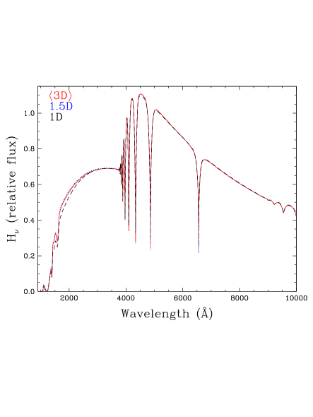
Figure 2: Predicted flux at $T_{\rm eff}=12,022$ K and $\log g=8$ based on a $\langle{\rm 3D}\rangle$ structure (solid, red), the 1.5D approximation (see text; blue, dotted) and a 1D ML2/$\alpha$ = 0.8 structure (black, dashed). All spectra were normalised at 4760 Å.

It is not straightforward to explain the physical reasons behind the correspondence between 3D and $\langle{\rm 3D}\rangle$ spectra. Kučinskas et al. (2013) studied 3D vs. $\langle{\rm 3D}\rangle$ effects for metal lines, but these results can not be applied to non-trace elements and saturated lines. In principle, the monochromatic flux would be best represented if $T^{4}$ was averaged over surfaces of constant $\tau_{\lambda}$ instead of one unique $\tau_{\rm R}$ scale. However, our results demonstrate that the mean monochromatic flux is well described by a single mean structure, which we traced back to the fact that the average over constant $\tau_{\rm R}$ provides a very good approximation of the mean monochromatic source function in the intensity forming layer

$$\langle S_{\lambda}(\tau)\rangle_{\tau_{\lambda}=1}\sim\langle S_{\lambda}(\tau)\rangle_{\tau_{\rm R}}(\langle\tau_{\lambda}\rangle=1)\leavevmode\nobreak\ ,$$ (1)

with

$${\rm d}\langle\tau_{\lambda}\rangle=-\langle\rho\rangle_{\tau_{\rm R}}\kappa_{\lambda}(\langle T^{4}\rangle_{\tau_{\rm R}}^{1/4},\langle P\rangle_{\tau_{\rm R}}){\rm d}\langle z\rangle_{\tau_{\rm R}}\leavevmode\nobreak\ ,$$ (2)

where $\rho$ is the density, $\kappa$ the opacity per gram and $P$ the pressure. We suggest that this behaviour is largely caused by a much more rapid variation of $\tau_{\rm R}$ as a function of geometrical depth in comparison to temperature. Hence, even if the $\tau_{\rm R}$ scale might not provide the best averaging surface, the resulting error on the mean monochromatic flux is very small for white dwarfs. We hope to develop this result more generally for all stellar types in a future work.

In terms of the temporal average, Ludwig (2006, see Eq. (56) and (59)) demonstrated that relative temporal variations of the box-averaged emergent flux scale approximately as

$$\frac{\sigma_{f}}{\langle f\rangle}\sim 0.5N_{\rm snapshot}^{-1/2}\frac{\delta I_{\rm rms}}{\langle I\rangle}\frac{l_{\rm gran}}{l_{\rm box}}\leavevmode\nobreak\ ,$$ (3)

where $\delta I_{\rm rms}/{\langle I\rangle}$ is the spatial relative intensity contrast (see Eq. (5) of Tremblay et al. 2013a) and $l_{\rm gran}/l_{\rm box}$ the linear dimension of one granule in box size units. The factor of $\sim$0.5 comes in part from the center-to-limb darkening and the fact that intensity is spatially correlated in granules. Given our simulations maximum intensity contrast of $\sim$20$\%$ (see Appendix A), it implies that the temporal flux variation is always less than 1% when we average 12 snapshots. Since we rely on normalised line profiles and not on the absolute flux, the impact on the predicted atmospheric parameters is significantly less than 1%.

The results of this section allow us, as in Paper II, to rely on the 1D spectral synthesis (and model atmosphere) code of Tremblay et al. (2011a) with the same microphysics as in our 3D simulations. We use $\langle T^{4}\rangle$ and $\langle P\rangle$ structures from 3D simulations as input to compute $\langle{\rm 3D}\rangle$ spectra, although populations and monochromatic opacities are recalculated in the spectral synthesis code. We also employ through this work 1D pure-hydrogen model spectra computed with the same code. These models are based, unless otherwise noted, on structures adopting the ML2/$\alpha$ = 0.8 parameterisation of the MLT. This calibration is established from a comparison of near-UV and optically determined $T_{\rm eff}$ (Tremblay et al. 2010), which we review in Sect. 3.3.

In Fig. 2, we compare normalised 1D and $\langle{\rm 3D}\rangle$ spectra at $T_{\rm eff}\sim 12,000$ K and $\log g=8$. The Fig. 16 of Paper II further highlights the differences in the wings of the Balmer lines. Clearly, the differences are fairly subtle and are mostly related to the shape of the line profiles. We have verified that there is no significant change in the predicted colours in the optical region. The flux in the wing of the Ly-$\alpha$ line, however, can be as much as 15% lower in the 1D case, although this depends on the employed MLT parameterisation. On the other hand, the absolute fluxes (not shown on the figure) are slightly offset due to 3D vs. $\langle{\rm 3D}\rangle$ effects, temporal averages, and the different radiative transfer routines in the 1D spectral synthesis and the 3D simulations.

3 Atmospheric parameters

The method used to derive atmospheric parameters from observed line profiles relies on the so-called spectroscopic technique developed by Bergeron et al. (1992). The first step is to normalise the flux from each individual Balmer line, typically from H$\alpha$ or H$\beta$ to H8, in both observed and model spectra, to a continuum set to unity at a fixed distance from the line center. The comparison with model spectra, which are convolved with the appropriate Gaussian instrumental profile, is then for these line profiles only. We rely on the same technique as the one described in Gianninas et al. (2011) to define the continuum of the observed spectra. In Fig. 3, we present an example of our fitting procedure for one cool star in the Gianninas et al. (2011) sample (see Sect. 4.1) with both the $\langle{\rm 3D}\rangle$ and 1D grid. The following sections provide a more detailed discussion of the differences between $\langle{\rm 3D}\rangle$ and 1D fits.

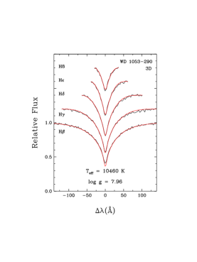
(a)

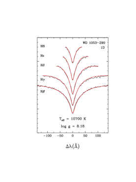
(b)

Figure 3: Simultaneous fit of the Balmer lines, from H$\beta$ to H8, for WD 1053$-$290 from the sample of Gianninas et al. (2011) by relying on $\langle{\rm 3D}\rangle$ (left panel) and 1D ML2/$\alpha$ = 0.8 (right panel) model spectra. Line profiles are offset vertically from each other for clarity and the best-fit atmospheric parameters are identified at the bottom of the panels. The instrumental resolution is of 6 Å. Line cores were partially removed from the $\langle{\rm 3D}\rangle$ fits (see Eq. (4)).

As a first step before using the $\langle{\rm 3D}\rangle$ spectra in spectroscopic analyses, we have to combine the $\langle{\rm 3D}\rangle$ grid with hotter and cooler 1D models since our 3D calculations do not cover the full range of $T_{\rm eff}$ for DA stars. We have created a combined grid of $\langle{\rm 3D}\rangle$ and 1D spectra in the range $6000<T_{\rm eff}$ (K) $<140,000$ and $\log g$ = 7.0, 7.5, 8.0, 8.5, and 9.0. We rely on $\langle{\rm 3D}\rangle$ spectra for $T_{\rm eff}$ up to 12,000, 12,500, 13,500, 14,000, and 14,500 K, for $\log g$ = 7.0, 7.5, 8.0, 8.5, and 9.0, respectively. The transition corresponds roughly to the position of the maximum strength of the H$\beta$ line. The next hotter model in the grid is a 500 K warmer 1D model. The justification for this transition is explained in Sect. 3.3. We note that the 1D models are identical to those used in Tremblay et al. (2011a), e.g. spectra derived from NLTE TLUSTY structures (Hubeny & Lanz 1995) are used for $T_{\rm eff}>$ 40,000 K.

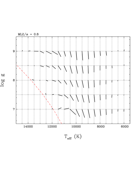
Figure 4: 3D atmospheric parameter corrections found by fitting our grid of $\langle$3D$\rangle$ spectra with the reference grid of 1D spectra relying on the ML2/$\alpha$ = 0.8 parameterisation of the MLT. The 1D = 3D reference parameters are on the intersection of the dotted lines, and 3D corrections are read by following the solid lines. We utilised a resolution of 3 Å and the cores of the deeper lines were removed from the fits (see Eq. (4)). The red dashed line represents the position of the maximum strength of the H$\beta$ line in the 1D models. Tabulated values are available in the online Appendix B.

Fig. 4 presents the 3D atmospheric parameter corrections found by fitting the $\langle{\rm 3D}\rangle$ spectra with our standard grid of 1D spectra. The 3D corrections were derived simultaneously for the five Balmer lines from H$\beta$ to H8 in the same way we fit observations. The line cores were partially removed from the fits, as well as the entire H$\alpha$ line, which is further discussed in Sect. 3.1. In the following sections, we study the 3D effects in more detail.

3.1 Line cores

The $\langle{\rm 3D}\rangle$ structures deviate significantly from their 1D counterparts in the upper layers ($\tau_{\rm R}<10^{-2}$) due to the cooling effect of convective overshoot. As demonstrated in Paper II, this results in deeper Balmer line cores for the $\langle{\rm 3D}\rangle$ spectra in comparison to the 1D case. The cooling effect is less significant for our hottest 3D simulations likely because the radiation field is stronger, although the impact on Balmer line cores is still substantial because the lines have their maximum strength near 13,500 K at $\log g=8$.

The $\langle{\rm 3D}\rangle$ line cores cause potential problems for spectroscopic analyses. First of all, it is not straightforward to combine the $\langle{\rm 3D}\rangle$ and 1D spectral grid since even the hottest 3D simulations still deviate from the 1D structures. Secondly, the predicted line cores of H$\alpha$ and H$\beta$ are systematically too deep compared to observations. For the typical case presented in Fig. 3, it is observed that while the overall quality of the fit is rather similar for the $\langle{\rm 3D}\rangle$ and 1D models, the H$\beta$ line core is too deep in the 3D case. The problem is more in evidence when the H$\alpha$ line is included.

We have no indication that our 3D simulations are inaccurate, and a similar dynamic cooling effect is predicted from 3D simulations of metal-poor dwarfs and giants computed with different codes (Asplund et al. 1999; González Hernández et al. 2010; Magic et al. 2013). In Paper II we have mentioned that missing NLTE effects are unlikely to cause a discrepancy in the line cores. The problem is also unlikely to be a direct effect of the limited number of opacity bins or the averaging procedure for $\langle{\rm 3D}\rangle$ structures. However, it is not excluded that the significant and simultaneous increase of the resolution, computation time, and number of opacity bins would lead to conditions of radiative equilibrium in the uppermost layers where the line cores are formed. Alternatively, the agreement of 1D spectra with observations could be a coincidence, implying that some physics is still missing from the models, e.g. magnetic fields amplified by convection or a proper line broadening theory for the line cores.

We have reviewed different ways of treating the line cores in the $\chi^{2}$ fitting procedure and found that the impact on 3D $\log g$ corrections is small. Best-fit surface gravities vary by less than $\sim$$|0.04|$ dex when a significant part of the line centers is removed, compared to overall 3D $\log g$ corrections reaching $\sim$$|0.20|$ dex. We found that the strongest effect of the cores is to shift $T_{\rm eff}$ values at the hot end of the 3D simulation sequence, near the position of the maximum strength of the Balmer lines. This is problematic in terms of combining the grid of $\langle{\rm 3D}\rangle$ spectra with hotter 1D models and it implies that the accuracy of 3D temperature determinations for $T_{\rm eff}\gtrsim 12,500$ K is only of the order of $\sim$250 K. For cooler models, 3D $T_{\rm eff}$ corrections are smaller, and become less dependent on the line cores.

In light of these experiments, we rely on the following parameterisation to remove the line centers from our $\langle{\rm 3D}\rangle$ fits. The line centers are removed when the following two conditions are verified.

$$|\Delta\lambda|\leavevmode\nobreak\ <1.0\leavevmode\nobreak\ \AA\leavevmode\nobreak\ \leavevmode\nobreak\ {\rm and}\leavevmode\nobreak\ \leavevmode\nobreak\ \frac{F_{\nu}}{F_{\nu,\leavevmode\nobreak\ \rm continuum}}=F_{\nu,\leavevmode\nobreak\ \rm normalised}<0.6$$ (4)

The latter requirement ensures that weak Balmer lines, such as higher lines or even the lower lines in very cool objects, are still taken into account. Furthermore, we have decided to neglect H$\alpha$ altogether. The line core problem is the most important for this line, and since it is situated in a different wavelength region with a different continuum flux, we find that it is better to remove the line altogether than use a more complex parameterisation to remove line cores. We employ Eq. (4) through this work except when we fit observed Balmer lines with 1D spectra in order to match published results.

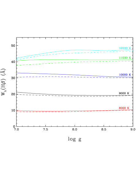
(a)

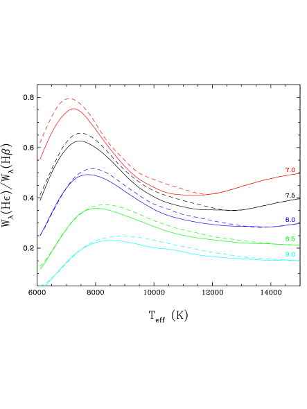
(b)

Figure 5: Left: Equivalent width of the H$\beta$ line for $\langle$3D$\rangle$ (solid line) and 1D (dashed) spectra as a function of $\log g$ for $T_{\rm eff}$ = 8000, 9000, 10,000, 11,000, and 12,000 K (values identified on the panel). Right: Ratio of the H$\epsilon$ and H$\beta$ equivalent widths as a function of $T_{\rm eff}$ for $\log g$ = 7.0, 7.5, 8.0, 8.5 and 9.0 (values identified on the panel). The line cores are not included in the equivalent width (see Eq. (4)).

3.2 3D effects

It was shown in Paper II that the differences are fairly subtle between the predicted $\langle{\rm 3D}\rangle$ and 1D spectra, and from that alone it is difficult to explain the 3D effects on the atmospheric parameters. From the comparison of the $\langle{\rm 3D}\rangle$ and 1D fits in Fig. 3, it is found that the fit quality is very similar, even though the best fit surface gravities are fairly different. Nevertheless, Fig. 4 demonstrates that 3D corrections show a well defined pattern in the HR diagram which we want to explain in this section. 3D corrections are mostly a function of $T_{\rm eff}$ with little influence from $\log g$ except for the hottest convective models.

Fig. 5 (left) presents the equivalent width of H$\beta$ as a function of $\log g$ for different $T_{\rm eff}$ values. It demonstrates that the strength of H$\beta$ is very sensitive to $T_{\rm eff}$, but is rather independent of $\log g$. The lower lines are therefore largely $T_{\rm eff}$ indicators in the convective regime. As a consequence, the convective overshoot cooling effect influencing the shape of the line cores for the lower Balmer lines mostly has an impact on 3D $T_{\rm eff}$ corrections.

On the right panel of Fig. 5, we show the ratio of the H$\epsilon$ and H$\beta$ equivalent widths as a function of $T_{\rm eff}$ for different surface gravities. It demonstrates that this ratio is rather sensitive to $\log g$ and to a lesser degree $T_{\rm eff}$. Furthermore, there are significant differences between the 3D and 1D cases, which largely explains the strong 3D $\log g$ corrections in Fig. 4. This is in agreement with the observation from Paper II that higher Balmer lines are more significantly impacted by 3D effects than lower lines. The reason for this behaviour is that the strength of the higher lines is more sensitive to the non-ideal effects (Hummer & Mihalas 1988; Tremblay & Bergeron 2009). These effects are in turn responsive to the density, and $\langle{\rm 3D}\rangle$ structures have systematically lower temperatures and higher densities in the formation region of the higher lines in the range $0.1<\tau_{\rm R}<1$ (see Fig. 7 of Paper II). Since increasing the surface gravity of a model also enhances the photospheric density, 3D effects are largely negative $\log g$ corrections.

The underlying reasons explaining the differences between $\langle{\rm 3D}\rangle$ and 1D structures in the formation region of the higher lines appear to be complex. The smaller temperature gradient in the 1D structures are caused by the fact that the 1D ML2/$\alpha$ = 0.8 parameterisation is more efficient than the 3D convection in that region. An explanation for this behaviour may not be possible until we have a general method to improve the 1D models to make them in close agreement with the $\langle{\rm 3D}\rangle$ structures. It is clear, however, that the 3D convective flux has a smoother profile as a function of depth in this transition region below the convective overshoot layer, while the 1D models have a rather sharp transition from convective to radiative conditions (see Fig. 9 of Paper II).

At the cool end of the sequence, both 1D and 3D structures are nearly fully adiabatic with a flat entropy profile from the bottom boundary and up to $\tau_{\rm R}\sim 10^{-2}$. While the 1D structures reach radiative equilibrium in the upper layers, 3D structures remain adiabatic (see Fig. 8 of Paper II). Since the 1D and 3D models are based on the same EOS, the adiabatic temperature structure is nearly identical in both cases. The hydrogen lines are fairly weak in this regime, hence the upper layers ($\tau_{\rm R}<10^{-2}$) have little effect on the predicted flux, and the 3D atmospheric parameter corrections are very small.

3.3 Calibration of the mixing-length theory

The 3D atmospheric parameter corrections in Fig. 4 are attached to the particular 1D reference grid, hence to the calibration of the choice of the MLT parameterisation. While Tremblay et al. (2010) suggest to rely on the ML2/$\alpha$ = 0.8 parameterisation, our results demonstrate that these 1D models are still significantly different to the 3D predictions, especially in terms of $\log g$ corrections. Recent analyses have employed 1D models based on the ML2/$\alpha$ = 0.6 parameterisation (see, e.g., Koester et al. 2009b; Kleinman et al. 2013), hence it is pertinent to compare the $\langle{\rm 3D}\rangle$ spectra with 1D models involving different MLT calibrations.

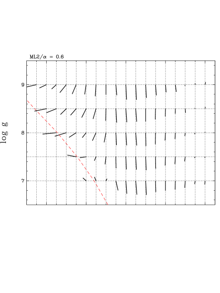
(a)

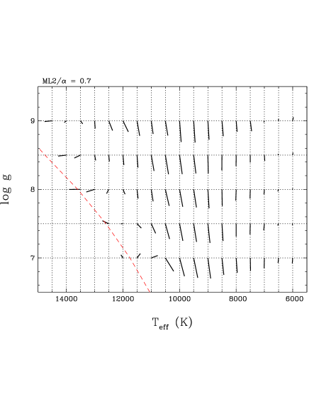
(b)

Figure 6: Similar to Fig. 4 but with a reference grid of 1D spectra relying on the ML2/$\alpha$ = 0.6 (top) and 0.7 (bottom) parameterisation of the MLT. Tabulated values are available in the online Appendix B.

In Fig. 6, we present 3D atmospheric parameter corrections with reference 1D grids relying on the ML2/$\alpha$ = 0.6 and 0.7 parameterisation. The $\log g$ corrections are similar in strength although the $T_{\rm eff}$ corrections are shifted. The ML2/$\alpha$ = 0.8 version provides the best match between $\langle{\rm 3D}\rangle$ and 1D spectra at the hot end of the sequence, although this result is sensitive to the parameterisation of Eq. (4). Nevertheless, the ML2/$\alpha$ = 0.6 definition renders an inferior match to the 3D results that can not be improved much by changing the line core removal procedure. At lower temperatures, 3D $T_{\rm eff}$ values are best matched with 1D models of lower convective efficiency, hence it appears that the MLT calibration may be a function of $T_{\rm eff}$ and $\log g$. In particular, in the range of the ZZ Ceti instability strip at $T_{\rm eff}\sim 12,000$ K, the ML2/$\alpha$ = 0.7 version provides $T_{\rm eff}$ values that are closer to the 3D results.

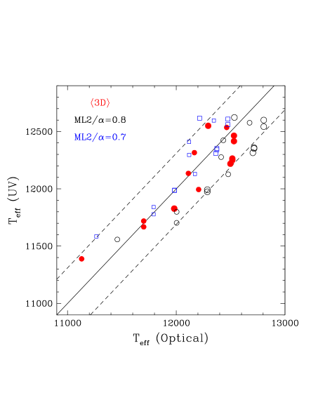
Figure 7: Comparison of $T_{\rm eff}$ for ZZ Ceti stars derived from near-UV spectra and compared with the optical determinations. Optical log g values are assumed in the determination of the UV temperatures. The size of the symbols reflects the different weights assigned to the UV spectra. The solid line represents a perfect match between UV and optical temperatures, while the dashed lines represent the $\sim$350 K uncertainty allowed by the optical analysis. We rely on the $\langle{\rm 3D}\rangle$ (red filled circles), 1D ML2/$\alpha$ = 0.8 (black open circles), and 1D ML2/$\alpha$ = 0.7 spectra (blue open squares). This is an updated version of Fig. 8 from Tremblay et al. (2010).

The MLT calibration for white dwarf model atmospheres has been historically performed from the comparison of effective temperatures measured independently from optical and near-UV spectra (Bergeron et al. 1995). The ML2/$\alpha$ = 0.6 parameterisation proposed by Bergeron et al. (1995) has been widely employed over the years. Tremblay et al. (2010) relied on the same technique to recalibrate the MLT to ML2/$\alpha$ = 0.8 in light of their new model atmospheres with the Tremblay & Bergeron (2009) Stark broadening calculations. The authors also found that the ML2/$\alpha$ $\sim$ 0.8 parameterisation produces the smoothest $\log g$ distribution as a function of $T_{\rm eff}$, i.e. without unexpected gaps or clumps of stars in observed samples, which is a further internal consistency check of the calibration.

We have updated the comparison of near-UV and optical parameters by using new optical spectra (Gianninas et al. 2011). The set of UV spectra comes from the Hubble Space Telescope (HST) and International Ultraviolet Explorer (IUE) near-UV observations (Holberg et al. 2003). We first fit the Balmer lines in the optical spectra to find $T_{\rm eff}$ (optical) and $\log g$ values. The atmospheric parameters cannot be fitted simultaneously in the near-UV continuum, hence we fix $\log g$ to the best-fit value in the optical, and then determine $T_{\rm eff}$ (UV) from the near-UV continuum. Fig. 7 demonstrates first of all that by relying on the most recent optical observations, the optimal ML2/$\alpha$ value appears to lie somewhere between 0.7 and 0.8 in this $T_{\rm eff}$ range. In the case of the $\langle{\rm 3D}\rangle$ spectra, the comparison of the optical and near-UV $T_{\rm eff}$ is not intended to calibrate the models but rather as an internal check of the accuracy of the 3D structures. It is very interesting to observe that $\langle{\rm 3D}\rangle$ spectra have consistent $T_{\rm eff}$ values in different wavelength regions. Since the near-UV flux at $T_{\rm eff}\sim 12,000$ K is formed relatively deep in the photosphere ($\tau_{\rm R}\sim$ 1) compared to the Balmer lines, it implies that the predicted structure of the photosphere is consistent with the observations.

In light of the above results, we must find a way to combine the grids of $\langle{\rm 3D}\rangle$ and 1D spectra. We observe that for ML2/$\alpha$ = 0.7 and 0.8 (Figs. 4 and 6), both $\log g$ and $T_{\rm eff}$ corrections are fairly small at the hot end of the 3D sequence, which would appear to confirm that our choice of a boundary is adequate. Since 3D $T_{\rm eff}$ corrections are sensitive to the line core removal procedure, we must be cautious about the significance of this agreement. We have chosen to make the connection at the $T_{\rm eff}$ which is approximately the closest to the maximum strength of the H$\beta$ line (red dashed line on Figs. 4 and 6 for 1D models). This is already a critical point in terms of line fitting since a small discrepancy in the predicted and observed maximum strength of Balmer lines ($\sim$1% in the equivalent width) causes gaps or clumps of stars in observed $\log g$ vs. $T_{\rm eff}$ distributions (Tremblay et al. 2011a). Furthermore, the $\chi^{2}$ fitting procedure often provides two valid solutions on both the hot and cool side of the maximum, hence it is difficult in any case to obtain precise atmospheric parameters in this region. The combination of the $\langle{\rm 3D}\rangle$ and 1D grids at this position allows to obtain smooth $\log g$ vs. $T_{\rm eff}$ distributions outside the transition regime.

3.4 3D atmospheric parameter correction functions

We have derived functions that can be used to convert spectroscopically determined 1D atmospheric parameters to their 3D counterparts. The recursive fitting procedure is detailed in Allende Prieto et al. (2013). Fortran 77 and IDL functions are available in the online Appendices C and D, respectively. One can also rely on the data from Figs. 4 and 6 given in the online Appendix B to derive alternative functions. Our independent variables are defined as

$$g_{\rm X}=\log g\leavevmode\nobreak\ {\rm[cgs]}-8.0\leavevmode\nobreak\ ,$$ (5)

$$T_{\rm X}=\frac{T_{\rm eff}\leavevmode\nobreak\ {\rm[K]}-10,000}{1000}\leavevmode\nobreak\ ,$$ (6)

and the fitting functions for the ML2/$\alpha$ = 0.7 (Eq. (7) and (8)) and 0.8 (Eq. (9) and (10)) parameterisation of the MLT are given below with the numerical coefficients identified in Table 1.

$$\frac{\Delta T_{\rm eff}}{1000}{\rm\leavevmode\nobreak\ [ML2/}\alpha\leavevmode\nobreak\ {\rm=0.7]}=a_{0}+[a_{1}+a_{4}T_{\rm X}+(a_{5}+a_{6}T_{\rm X}+a_{7}g_{\rm X})g_{\rm X}]\exp[-a_{2}(T_{\rm X}-a_{3})^{2}]\leavevmode\nobreak\ ,$$ (7)

$$\Delta\log g{\rm\leavevmode\nobreak\ [ML2/}\alpha\leavevmode\nobreak\ {\rm=0.7]}=b_{0}+b_{1}\exp\left\{-\big{(}b_{2}+(b_{4}+b_{6}\exp[-b_{7}(T_{\rm X}-b_{8})^{2}])T_{\rm X}+(b_{5}+b_{9}T_{\rm X}+b_{10}g_{\rm X})g_{\rm X}\big{)}^{2}(T_{\rm X}-b_{3})^{2}\right\}\leavevmode\nobreak\ .$$ (8)

$$\frac{\Delta T_{\rm eff}}{1000}{\rm\leavevmode\nobreak\ [ML2/}\alpha\leavevmode\nobreak\ {\rm=0.8]}=c_{0}+(c_{1}+c_{6}T_{\rm X}+c_{7}g_{\rm X})\exp[-(c_{2}+c_{4}T_{\rm X}+c_{5}g_{\rm X})^{2}(T_{\rm X}-c_{3})^{2}]\leavevmode\nobreak\ ,$$ (9)

$$\Delta\log g{\rm\leavevmode\nobreak\ [ML2/}\alpha\leavevmode\nobreak\ {\rm=0.8]}=\big{(}d_{0}+d_{4}\exp[-d_{5}(T_{\rm X}-d_{6})^{2}]\big{)}+d_{1}\exp\left\{-d_{2}\big{[}T_{\rm X}-(d_{3}+d_{7}\exp(-[d_{8}+d_{10}T_{\rm X}+d_{11}g_{\rm X}]^{2}[T_{\rm X}-d_{9}]^{2}))\big{]}^{2}\right\}\leavevmode\nobreak\ .$$ (10)

Table 1: Coefficients for fitting functions

Coeff.	$\Delta T_{\rm eff}$ [ML2/$\alpha$ = 0.7]	Coeff.	$\Delta\log g$ [ML2/$\alpha$ = 0.7]
$a_{0}$	$-$1.0461690E$-$03	$b_{0}$	1.1922481E$-$03
$a_{1}$	$-$2.6846737E$-$01	$b_{1}$	$-$2.7230889E$-$01
$a_{2}$	3.0654611E$-$01	$b_{2}$	$-$6.7437328E$-$02
$a_{3}$	1.8025848E+00	$b_{3}$	$-$8.7753624E$-$01
$a_{4}$	1.5006909E$-$01	$b_{4}$	1.4936511E$-$01
$a_{5}$	1.0125295E$-$01	$b_{5}$	$-$1.9749393E$-$01
$a_{6}$	$-$5.2933335E$-$02	$b_{6}$	4.1687626E$-$01
$a_{7}$	$-$1.3414353E$-$01	$b_{7}$	3.8195432E$-$01
…	…	$b_{8}$	$-$1.4141054E$-$01
…	…	$b_{9}$	$-$2.9439950E$-$02
…	…	$b_{10}$	1.1908339E$-$01
Coeff.	$\Delta T_{\rm eff}$ [ML2/$\alpha$ = 0.8]	Coeff.	$\Delta\log g$ [ML2/$\alpha$ = 0.8]
$c_{0}$	1.0947335E$-$03	$d_{0}$	7.5209868E$-$04
$c_{1}$	$-$1.8716231E$-$01	$d_{1}$	$-$9.2086619E$-$01
$c_{2}$	1.9350009E$-$02	$d_{2}$	3.1253746E$-$01
$c_{3}$	6.4821613E$-$01	$d_{3}$	$-$1.0348176E+01
$c_{4}$	$-$2.2863187E$-$01	$d_{4}$	6.5854716E$-$01
$c_{5}$	5.8699232E$-$01	$d_{5}$	4.2849862E$-$01
$c_{6}$	$-$1.0729871E$-$01	$d_{6}$	$-$8.8982873E$-$02
$c_{7}$	1.1009070E$-$01	$d_{7}$	1.0199718E+01
…	…	$d_{8}$	4.9277883E$-$02
…	…	$d_{9}$	$-$8.6543477E$-$01
…	…	$d_{10}$	3.6232756E$-$03
…	…	$d_{11}$	$-$5.8729354E$-$02

Our fitting functions provide negligible 3D corrections for DA white dwarfs with $T_{\rm eff}$ values outside the range of our 3D simulations. We are also aware that our 3D grid does not extend to high and low enough gravities to cover some of the most extreme and interesting white dwarf observations (see, e.g., Kepler et al. 2007; Hermes et al. 2013). However, our fitting functions should be able to provide reasonable estimates since 3D parameter corrections are, in most cases, fairly regular as a function of $\log g$, except for the transition region between convective and radiative atmospheres.

We do not provide a function for ML2/$\alpha$ = 0.6 since the connection of our $\langle{\rm 3D}\rangle$ spectra with hotter 1D spectra is problematic. We suggest instead that 1D models with ML2/$\alpha$ = 0.7 or 0.8 should be used. Nevertheless, we provide tabulated values of the 3D corrections for ML2/$\alpha$ = 0.6 in the Appendix B.

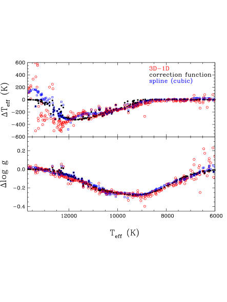
Figure 8: 3D vs. 1D $T_{\rm eff}$ (top) and $\log g$ (bottom) from actual 3D and 1D fits (red open circles) and by using our correction function (Eq. (9) and (10)) to modify the 1D parameters (black filled circles). We also employ a cubic spline interpolation of the 3D corrections (blue open squares) to modify the 1D parameters.

In Fig. 8, we compare $T_{\rm eff}$ and $\log g$ values for the Gianninas et al. (2011) sample (see Sect. 4.1) found by fitting directly the observations with our $\langle{\rm 3D}\rangle$ and 1D spectra and from converting the 1D parameters using our fitting functions (Eq. (9) and (10)). As a reference, we also convert the 1D parameters by employing a cubic spline interpolation with the data from Fig. 4. This method preserves more details compared to our fitting functions. We note that additional sequences at $\log g=$ 7.75 and 8.25 are part of the 1D grid and that line cores are not removed from the 1D fits. Nevertheless, it is shown that the atmospheric parameters are fairly similar in all cases, and that our fitting functions are adequate to provide precise 3D parameters. We have chosen fitting functions that do not preserve all details of the 3D $T_{\rm eff}$ corrections unlike, for instance, the spline interpolation. This choice was made because the small scale fluctuations are below the model (e.g. line core removal procedure) and observational uncertainties, and it would be difficult to justify that they are real physical features.

At the hot end of the sequence, there are some discrepancies in the $T_{\rm eff}$ values found from fits with $\langle{\rm 3D}\rangle$ spectra and tabulated corrections (with either the spline interpolation or fitting functions). We believe that the 3D corrections drawn from Fig. 4 smooth out some of the issues obtained with the monochromatic flux interpolation in the predicted spectra. The latter is difficult to perform in this range of $T_{\rm eff}$ because the wavelength regions close to the line cores are predicted differently in the 1D and $\langle{\rm 3D}\rangle$ spectra. At the cool end of the sequence, it appears that the line core removal procedure enhances the scatter in the $\langle{\rm 3D}\rangle$ fits. In light of these results, we have decided to rely on the correction functions (Eq. (9) and (10)) for the rest of this work.

4 Astrophysical implications

In order to study the astrophysical implications of our improved predicted spectra for convective DA white dwarfs, we have chosen to review the properties of two well studied samples, that of the White Dwarf Catalog (McCook & Sion 1999) and the Sloan Digital Sky Survey (York et al. 2000, hereafter SDSS). In particular, we base our study on the spectroscopic analyses of Gianninas et al. (2011, hereafter GB11) for the White Dwarf Catalog and Tremblay et al. (2011a, hereafter TB11) for the SDSS, where the sample is derived from the Data Release 4. The advantage of these studies is that they rely on the same 1D model atmospheres (ML2/$\alpha$ = 0.8) and the same fitting method as we use in this work. Furthermore, in both cases the authors made a thoughtful examination of the data in order to identify subtypes, such as binaries and magnetic white dwarfs. This allows for a better precision in the determination of the mean properties of the samples. While both surveys have been enlarged with newly observed DA white dwarfs (Kleinman et al. 2013, and A. Gianninas, private communication), we believe that our selected samples are large and complete enough to study the 3D effects on the predicted atmospheric parameters.

We convert $\log g$ values into stellar masses using the evolutionary models with thick hydrogen layers of Fontaine et al. (2001) below $T_{\rm eff}<$ 30,000 K and of Wood (1995) above this temperature. Low-mass white dwarfs, below 0.46 $M{{}_{\odot}}$ and $T_{\rm eff}<$ 50,000 K, are likely helium core white dwarfs, and we rely instead on evolutionary models from Althaus et al. (2001). For masses higher than 1.3 $M{{}_{\odot}}$, we use the zero temperature calculations of Hamada & Salpeter (1961).

4.1 White Dwarf Catalog sample

We review the mass distribution of the Gianninas et al. (2011) sample of 1265 bright DA white dwarfs ($V\lesssim 17.5$) drawn from the online version of the McCook & Sion White Dwarf Catalog (hereafter WDC). High S/N observations ($\langle{\rm S/N}\rangle$ $\sim$ 70) were secured for all objects in the sample over a period of $\sim$20 years at different sites (see Sect. 2 of GB11). Therefore, observations in the GB11 sample do not have a homogeneous instrumental setup, with a resolution varying from $\sim$3 to 12 Å (FWHM). Our starting point are the objects identified in Table 5 of GB11. We rely on the same observations and the same grid of 1D model atmospheres to determine the atmospheric parameters. We took their solutions for DAO and hot DA white dwarfs with the Balmer-line problem (Werner 1996) where they employed NLTE models with carbon, nitrogen and oxygen (Gianninas et al. 2010). The addition of these elements has a cooling effect on the upper layers and the predicted line cores are in better agreement with the observations. Therefore, our analysis only differs from that of GB11 considering that we also derive 3D atmospheric parameters.

Figure 9: $\log g$ versus $T_{\rm eff}$ distribution for DA white dwarfs in the GB11 sample derived from $\langle$3D$\rangle$ (top) and 1D spectra (bottom). An evolutionary model from Fontaine et al. (2001) at the median mass of the sample (0.61 $M_{\odot}$, $13,000<T_{\rm eff}$ (K) $<40,000$) is shown as a dashed line. The error bars on the top left represent the mean uncertainties in this $T_{\rm eff}$ range.

Figure 10: Mass versus $T_{\rm eff}$ (logarithm scale) distribution for DA white dwarfs in the GB11 sample derived from $\langle$3D$\rangle$ (top) and 1D spectra (bottom). Lines of constant mass at 0.55 $M{{}_{\odot}}$ and 0.7 $M{{}_{\odot}}$ are shown as a reference.

We present in Fig. 9 and 10 the GB11 sample $\log g$ and mass distributions as a function of $T_{\rm eff}$ employing either 1D or 3D model atmospheres. The distributions are identical for radiative atmospheres ($T_{\rm eff}\gtrsim 15,000$ K). The distributions relying on $\langle{\rm 3D}\rangle$ spectra are much more stable as a function of $T_{\rm eff}$ and the high-$\log g$ problem is to a very large extent removed. Nevertheless, masses at $T_{\rm eff}\sim 12,000$ K appear slightly larger than the sample average. We review this issue more quantitatively in Sect. 5.

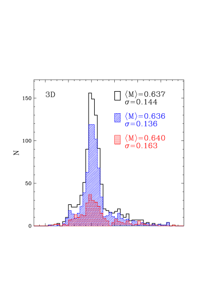
(a)

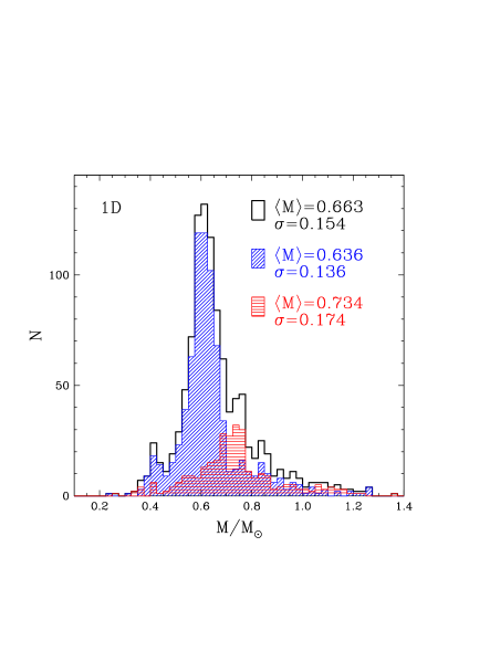
(b)

Figure 11: Top: Mass histogram for DA stars in the GB11 sample with $T_{\rm eff}<$ 40,000 K (black empty histogram) from $\langle$3D$\rangle$ spectra. We also show the sub-distributions for $13,000<T_{\rm eff}$ (K) $<40,000$ (blue histogram, dashed diagonally, radiative atmospheres) and $T_{\rm eff}<13,000$ K (red histogram, dashed horizontally, convective atmospheres). The number of stars is given on the left-hand scale. The mean masses and standard deviations are indicated in the panels in units of solar masses. Binaries and magnetic objects were removed from the distributions. Bottom: Same as above but with 1D spectra.

The mass histograms for the GB11 sample using both 1D and 3D models are shown in Fig. 11. We have restricted the analysis to objects below $T_{\rm eff}<40,000$ K for an easier comparison with the SDSS sample even though hot white dwarfs in the GB11 sample have accurate atmospheric parameters. Furthermore, we have removed all objects identified as binaries, including DA+dM composite spectra and double degenerates, and objects with evidences of Zeeman splitting. These subtypes typically have larger uncertainties on their atmospheric parameters and appear to have different mass distributions than typical single DAs, either due an observational bias or intrinsic properties (Kawka et al. 2007; TB11). We have used a threshold at 13,000 K to separate between the regime of radiative (blue colour in Fig. 11) and convective (red) atmospheres. The 1D mean masses for convective and radiative white dwarfs have a significant offset of $\Delta M/M{{}_{\odot}}$ = +0.10, which is largely corrected by the 3D models, where the offset is not significant. The properties of the standard deviation are discussed in Sect. 5.

4.2 Sloan Digital Sky Survey

We rely on the sample of Eisenstein et al. (2006) drawn from the Data Release 4 of the SDSS, which has been reviewed in numerous studies (Kepler et al. 2007; De Gennaro et al. 2008, and TB11). In particular, our starting point are the 3072 DA stars in Table 1 of TB11, who improved upon previous analyses by including the Stark broadening profiles of Tremblay & Bergeron (2009) and by performing a careful visual inspection to identify subtypes and calibration problems. In the following, we identify this sample as E06/TB11. We note that the Kleinman et al. (2013) sample drawn from the DR7 approximately doubles the size of the previous Eisenstein et al. (2006) sample. The Kleinman et al. (2013) analysis relies on different 1D model atmospheres, fitting procedures and manual inspection methods to identify subtypes. While their study should be equivalent to that of TB11, we would need first of all to compare both approaches, which is out of the scope of this work.

White dwarf spectra in the sample of Eisenstein et al. (2006) were identified from a combination of the object $ugriz$ colours, the absence of a redshift, and an automated comparison of the photometric and spectroscopic data with white dwarf models. These steps are quite robust in recovering most single DA white dwarfs with $T_{\rm eff}\gtrsim 8000$ K observed spectroscopically by the SDSS. However, the completeness of the SDSS spectroscopic survey itself can be anywhere between 15% and 50%, in part due to the neglect of blended point sources, as well as an incomplete spectroscopic follow-up of the point sources identified in the SDSS fields (Eisenstein et al. 2006; De Gennaro et al. 2008; Kleinman et al. 2013).

TB11 found that a cutoff at S/N $>15$, which we also apply here, allowed for the best compromise between the size of the sample and the precision of its mean properties. The sole difference in comparison to the TB11 analysis is that we rely on the most recent DR9 data reduction, instead of the one from DR7, for both the spectroscopic and photometric data obtained from the SDSS DR9 Science Archive Server and Sky Server. The spectra, which cover a wavelength range of 3800 to $\sim$10,000 Å with a resolution of $R\sim 1800$, appeared to have some calibration issues up to the DR7 (Kleinman et al. 2004; Eisenstein et al. 2006; TB11; GB11). For a sample of 89 stars observed by both the SDSS and GB11, the Fig. 17 of TB11 highlights a systematic $\log g$ difference between both data sets. Since the models and the fitting procedure are identical, differences must lie in the observations. This issue is mostly seen for hot white dwarfs and given the available objects in common, the samples are roughly in agreement within the uncertainties for cool convective objects. Nevertheless, we feel that it is especially important to rely on the latest data reduction.

Figure 12: $\log g$ versus $T_{\rm eff}$ distribution for DA white dwarfs with S/N $>$ 15 in the SDSS E06/TB11 sample derived from $\langle$3D$\rangle$ (top) and 1D (bottom) spectra. An evolutionary model from Fontaine et al. (2001) at the median mass of the sample (0.59 $M_{\odot}$, $13,000<T_{\rm eff}$ (K) $<40,000$) is shown as a dashed line. The error bars on the top left represent the mean uncertainties in this $T_{\rm eff}$ range.

Figure 13: Mass versus $T_{\rm eff}$ distribution for DA white dwarfs in the SDSS E06/TB11 sample derived from $\langle$3D$\rangle$ (top) and 1D spectra (bottom). Lines of constant mass at 0.55 $M{{}_{\odot}}$ and 0.7 $M{{}_{\odot}}$ are shown as a reference.

In Fig. 12 and 13 we present the $\log g$ and mass distributions as a function of $T_{\rm eff}$ for the SDSS E06/TB11 sample (S/N $>15$) with both the 1D and $\langle{\rm 3D}\rangle$ spectra. For cooler convective objects, the 1D $\log g$ distribution illustrates the classic high-$\log g$ problem with a significant downturn. The problem is largely removed from the distribution relying on 3D model atmospheres. Nevertheless, the mass distribution still shows some substructures with masses that appear too high at $T_{\rm eff}\sim 12,000$ K, similarly to what is observed for the GB11 sample.

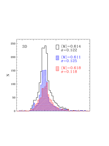
(a)

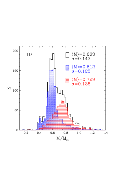
(b)

Figure 14: Similar to Fig. 11 but for the SDSS E06/TB11 sample with $T_{\rm eff}<$ 40,000 K and S/N $>$ 15 (black empty histograms). We also highlight the sub-distributions for $13,000<T_{\rm eff}$ (K) $<40,000$ (blue histograms, radiative atmospheres) and $T_{\rm eff}<13,000$ K (red histograms, convective atmospheres). Binaries and magnetic objects were removed from the distributions.

As in TB11, we restrict our determination of the mean mass to objects with $T_{\rm eff}<40,000$ K. This cutoff is applied in part because it is difficult to identify metal-rich objects with the Balmer-line problem at the low average S/N of the SDSS observations. Furthermore, we remove all identified binaries and magnetic objects. Fig. 14 includes mass histograms for both the hot radiative (blue, $T_{\rm eff}>13,000$ K) and cool convective (red, $T_{\rm eff}<13,000$ K) atmospheres. The first observation is that the mass distribution of hot radiative white dwarfs is nearly identical to the one found in TB11 using the DR7 instead of the DR9 data reduction. The 1D mass distribution below $T_{\rm eff}$ = 13,000 K has a significantly higher mean value, with $\Delta M/M{{}_{\odot}}$ = +0.12. In the case of the 3D mass distributions, this shift decreases to a value of +0.01. This outcome is very similar to that of the GB11 sample.

4.3 Photometric samples

Photometric observations of white dwarfs allow for the determination of independent $T_{\rm eff}$ values (Koester et al. 1979). When trigonometric parallax measurements are available, it is also possible to constrain $\log g$ (Bergeron et al. 2001). Since our $\langle{\rm 3D}\rangle$ spectra predict roughly the same optical colours as the 1D models, earlier photometric studies are unchanged and we can compare directly these results to our spectroscopic parameters.

Koester et al. (2009a) and Tremblay et al. (2010) have reviewed the current photometric constraints on the atmospheric parameters of convective DAs with the perspective of finding a solution to the high-$\log g$ problem. We can therefore use their studies as a starting point. There is currently a lack of parallax samples that are both precise and large. Therefore, Tremblay et al. (2010) concluded that the parallax and $VRIJHK$ photometric sample of eight DA stars from Subasavage et al. (2009) provided the most precise independent constraint on the individual masses of cool DA stars. In Fig. 15, we update the Fig. 12 of Tremblay et al. (2010) by presenting a comparison of the photometric and spectroscopic parameters relying on both the 3D and 1D model atmospheres. The masses found from parallaxes are now in much better agreement with those found spectroscopically by using $\langle{\rm 3D}\rangle$ spectra. However, given the small size of the sample and possible differences in the internal composition of those white dwarfs influencing the mass-radius relation, it is difficult to conclude further on the accuracy of the 3D model atmospheres.

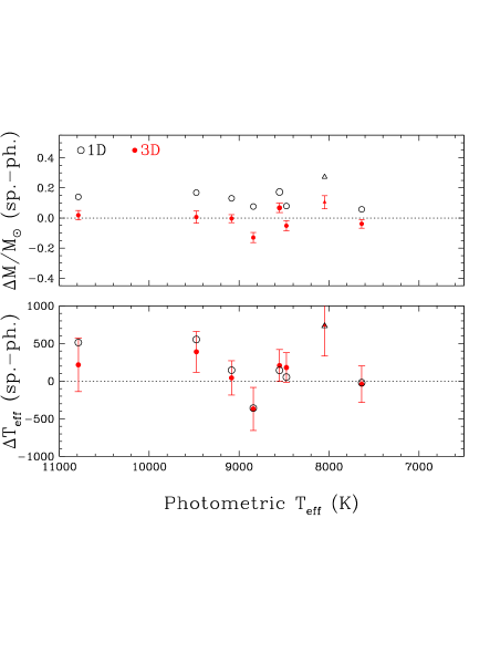
Figure 15: Comparison of the photometric and spectroscopic masses (top) and $T_{\rm eff}$ (bottom) for DA white dwarfs in the Subasavage et al. (2009) sample. We rely on both $\langle$3D$\rangle$ (filled red circles and error bars) and 1D (open black circles) spectra. The error bars are omitted in the 1D case for clarity. The object represented by a triangle (LHS 4040) possibly has some contamination from a nearby M dwarf. The horizontal dotted lines correspond to a perfect match between spectroscopic and photometric parameters. This is an updated version of Fig. 12 from Tremblay et al. (2010).

The photometric data also offers an unique opportunity to independently measure $T_{\rm eff}$ values. In the case of the Subasavage et al. (2009) sample, Fig. 15 shows that photometric and spectroscopic $T_{\rm eff}$ are in a slightly better agreement in 3D. However, the mixing-length parameter in the 1D models could be updated to provide a closer agreement with the 3D values.

The $ugriz$ energy distribution is available for most SDSS objects in our sample, and for convective objects, the predicted magnitudes are rather sensitive to $T_{\rm eff}$, allowing for a precision on the photometric $T_{\rm eff}$ of the order of 5$\%$. Since parallaxes are not available, it is not possible to individually constrain $\log g$ values. Fig. 16 compares the spectroscopic and photometric $T_{\rm eff}$ for both the 1D and 3D model atmospheres. To prevent uncertainties due to reddening, we only include objects with $g<18$. Fig. 16 demonstrates that 3D spectroscopic $T_{\rm eff}$ are in reasonable agreement with the photometric values. Since both the spectroscopic and photometric SDSS data may be impacted by calibration issues, it is difficult to conclude on the accuracy of 3D $T_{\rm eff}$ corrections from this comparison. Nevertheless, the results of this section, along with the comparison of optical and near-UV $T_{\rm eff}$ in Sect. 3.3, illustrate that the corrections are certainly acceptable. A dedicated survey of high-precision photometry and parallaxes for cool DA white dwarfs would help in further understanding the accuracy of the model atmospheres.

Figure 16: Comparison of photometric and spectroscopic $T_{\rm eff}$ for DA white dwarfs in the SDSS E06/TB11 sample relying on $\langle$3D$\rangle$ (top) and 1D (bottom) spectra. The mean uncertainty is shown with error bars on the top panel.

5 Discussion

We have described in this work the effects of 3D model atmospheres on the determination of the atmospheric parameters of DA white dwarfs. Our proposed 3D $\log g$ corrections are in agreement with those found in our previous study limited to $\log g=8$ (Paper II). We have shown that the mass distribution of radiative and convective atmosphere white dwarfs are now in quantitative agreement. We have confirmed the results of earlier studies that 1D model atmospheres relying on the MLT are responsible for the high-$\log g$ problem and that 3D model atmospheres do not have this shortcoming. It demonstrates clearly that one should rely on 3D model atmospheres, or 1D model atmospheres with 3D correction functions, to have a precision higher than $\sim$10-20% on the mass and age of convective DA stars. In this section, we attempt to further characterise the accuracy of our current grid of $\langle$3D$\rangle$ spectra by comparing the results found for the SDSS E06/TB11 and Gianninas et al. (2011) samples.

5.1 Accuracy of the $\langle$3D$\rangle$ spectra

It is not straightforward to compare the SDSS E06/TB11 and GB11 samples in terms of the absolute value of the mean mass and the related standard deviation. In addition to possible issues with the data calibration, the samples have significantly different selection criteria and completeness levels (Eisenstein et al. 2006; GB11). The SDSS sample is mostly magnitude-limited while stars identified in the White Dwarf Catalog are drawn from various surveys, including X-ray surveys like the one conducted with ROSAT which is not magnitude limited. Since high-mass white dwarfs are fainter, it is perhaps not surprising that the White Dwarf Catalog sample includes more massive objects than the SDSS, possibly explaining the higher mean mass. The mass dispersion is also significantly higher for the GB11 sample, perhaps also due to the presence of a larger number of high-mass objects, but it is suspected that the different instrumental setup and data reduction have an impact as well.

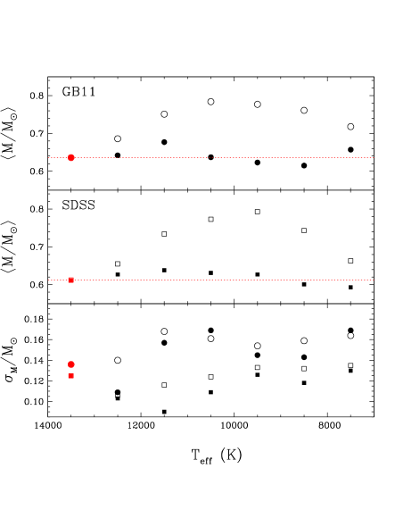
Figure 17: Mean mass (top panels) and standard deviation (bottom panel) computed in 1000 K temperature bins for the GB11 (circles, top panel) and SDSS E06/TB11 (squares, middle panel) samples. Values are derived from both $\langle$3D$\rangle$ (filled circles) and 1D spectra (open circles). The red circles on the left and the dotted lines represent the values for hotter radiative objects ($13,000<T_{\rm eff}$ (K) $<40,000$).

In Fig. 17, we compare the mass distributions of the SDSS E06/TB11 and GB11 samples (Figs. 10 and 13) in bins of 1000 K to better understand mean mass fluctuations. As a reference, the mean mass in the range $13,000<T_{\rm eff}$ (K) $<40,000$ is shown by red circles and dotted lines. We see that in terms of the mean mass, both samples show a similar variation as a function of $T_{\rm eff}$. In the 3D case, there is a clear increase in the $11,000<T_{\rm eff}$ (K) $<12,000$ bin for both surveys. We currently have no explanation for this behaviour. We have verified that changes in the parameterisation of the line core removal do little to improve the situation. While the reason might be the inaccuracy of our first grid of 3D model atmospheres, we could also be observing some issues with the spectral synthesis, e.g. from the opacities or EOS, that were previously hidden behind the high-$\log g$ problem.

The variation of the mass standard deviation as a function of $T_{\rm eff}$ (bottom panel of Fig. 17) has a rather complex behaviour. The overall lower values in the 3D case simply reflect the fact that the gravities are smaller, hence also the mass range. The increase of the dispersion at low $T_{\rm eff}$, especially in the case of the SDSS sample, is likely related to the fact that lines are weaker and that the mean $\log g$ error increases. The minima in the standard deviation at $T_{\rm eff}\sim$ 11,500-12,500 K are more difficult to explain. This could be due to incorrect 3D $T_{\rm eff}$ corrections, especially for the low- and high-mass objects which could be systematically shifted to another bin.

For cool convective white dwarfs ($T_{\rm eff}\lesssim 8000$ K), neutral broadening and related non-ideal effects due to neutral particles become dominant for the Balmer lines. In their discussion of the high-$\log g$ problem, Tremblay et al. (2010) mention how the uncertainties in neutral broadening and the Hummer & Mihalas (1988) theory for non-ideal perturbations (hard sphere model) may impact the model predictions. In particular, Bergeron et al. (1991) found that $\log g$ values are too low in the regime where non-ideal effects become dominated by neutral interactions, hence they divided the hydrogen radius by a factor of 2 in the Hummer & Mihalas hard sphere formalism. While it is now clear that these uncertainties are not the source of the high-$\log g$ problem, they may impact the spectroscopic mass distributions for $T_{\rm eff}\lesssim 8000$ K. The 3D mass distributions in Fig. 17 remain relatively stable as a function of $T_{\rm eff}$ for the coolest white dwarfs. Our results suggest that the current parameterisation of the non-ideal effects due to neutral interactions does not need to be revised for the 3D effects. Finally, it is worth mentionning that our assumption of thick H layers for all DA white dwarfs also has a slight effect on our results. Considering that most ($\gtrsim 80\%$) DAs appear to have thick layers (Tremblay & Bergeron 2008), we expect an offset below $1\%$ on the derived mean masses.

5.2 ZZ Ceti white dwarfs

We present in this section a brief study of the pulsating ZZ Ceti properties as seen in the light of 3D model atmospheres. Our starting point is once again the sample of GB11 for which they made a distinction between pulsating, photometrically constant and unconstrained objects. In the latter case, the stars were not observed to detect possible light variations. In their Fig. 33, GB11 have studied the position of the ZZ Ceti instability strip relying only on the stars in their sample that have been observed for photometric variability. Their purpose was to update the position of the instability strip given the improved 1D model atmospheres of Tremblay & Bergeron (2009) and the resulting change in the MLT calibration from ML2/$\alpha$ = 0.6 to 0.8. We propose here a very similar study with our improved 3D model atmospheres.

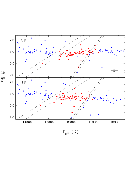
Figure 18: Surface gravity versus $T_{\rm eff}$ distribution for ZZ Ceti (circles, red) and photometrically constant (squares, blue) DA white dwarfs in the Gianninas et al. (2011) sample with $\langle$3D$\rangle$ (top) and 1D (bottom) spectra. The dotted lines are the ZZ Ceti instability strip boundaries established by Gianninas et al. (2006) while the dashed lines are the most recent boundaries identified by Gianninas et al. (2011) relying on the models from Tremblay & Bergeron (2009). The error bars represent the average uncertainties of the spectroscopic method in the region of the ZZ Ceti instability strip.

In Fig.18, we present the $\log g$ distribution of the GB11 sample in the region of the ZZ Ceti instability strip and identify photometrically variable and constant objects. For reference, we also add the observed red and blue edges of the instability strip as determined by GB11 (ML2/$\alpha$ = 0.8, dashed lines). We remind the reader that while the observed edges depend on the predicted Balmer lines and the model atmospheres, the MLT parameterisation (see Sect. 3.3) is independent of asteroseismic predictions. The $T_{\rm eff}$ and $\log g$ shifts are moderate in this regime, hence the position and shape of the instability strip with $\langle$3D$\rangle$ spectra are not dramatically different in comparison to the 1D ML2/$\alpha$ = 0.8 parameterisation. The blue and red edge appear to be slightly cooler. Furthermore, the purity of the instability strip and the sharpness of the edges are not modified because the 3D corrections have a largely systematic behaviour.

We note that recent theoretical determinations of the blue and red edge positions from asteroseismology (Fontaine & Brassard 2008; Córsico et al. 2012; van Grootel et al. 2012, 2013) are in agreement with the GB11 or earlier Gianninas et al. (2006) observed positions. It is encouraging that the observed 3D boundaries are also in agreement with asteroseismology, although 3D $T_{\rm eff}$ corrections around $12,500$ K are sensitive to the line cores, hence our results for ZZ Ceti stars should be taken with some caution. Furthermore, asteroseismic models rely on 1D structure models (typically under the ML2/$\alpha$ = 1.0 parameterisation) and it is currently unknown how much the 3D model atmospheres would impact the results. In addition to different convective efficiencies between the 1D and 3D models leading to distinctive sizes for the convective zone, the 3D simulations show overshoot layers at the bottom of the convective zone which are missing from the 1D models.

6 Conclusion

We presented a new grid of spectra for DA white dwarfs drawn from CO⁵BOLD 3D radiation-hydrodynamics simulations. The 3D effects on the atmospheric parameters of DA stars have been studied for the SDSS and White Dwarf Catalog spectroscopic samples (Tremblay et al. 2011a; Gianninas et al. 2011). We found that the mean spectroscopic mass of cool convective white dwarfs is significantly lower, by about $\sim$0.10 $M{{}_{\odot}}$, when we rely on 3D instead of 1D model atmospheres. The mean mass of objects with hot radiative and cool convective atmospheres is now roughly the same for both spectroscopic samples. This is in much better agreement with independent parallax observations and our knowledge of stellar evolution. We have proposed correction functions that can be used to convert spectroscopically determined 1D atmospheric parameters to 3D values. The 3D atmospheric parameters can then be utilised to determine improved values of the mass, age, and population membership for convective DA white dwarfs.

We found that 3D $T_{\rm eff}$ corrections are small, and that they are in agreement with photometric and near-UV determined $T_{\rm eff}$ values. We nevertheless noted some shortcomings of the current grid of $\langle$3D$\rangle$ spectra. The masses are predicted slightly too high ($\sim$5%) at $T_{\rm eff}\sim 12,000$ K and $T_{\rm eff}$ corrections are also uncertain in this regime ($\pm$250 K). These issues might not only be related to the 3D simulations, but also to shortcomings in the predicted line profiles that were previously hidden behind the high-$\log g$ problem.

We demonstrated that the observed ZZ Ceti instability strip remains at a very similar position in the HR diagram compared to previous determinations with 1D spectra. We hope, however, that our 3D atmospheres can also be implemented as the upper boundary of white dwarf structure calculations, for instance by using the methods of Gautschy et al. (1996) and Ludwig et al. (1999). This would allow the asteroseismic applications to also benefit from an improved model of convection, and to determine whether there is an impact on the theoretical position of the ZZ Ceti instability strip.

Appendix A Supplementary data I

Table 2: Grid of CO⁵BOLD 3D model atmospheres for DA white dwarfs

$T_{\rm eff}$	$\log g$	$\log z$	$\log x$	$\log$ Char. size	$\log\tau_{\rm R,min}$	$\log\tau_{\rm R,max}$	$\ln(P_{\rm bot}/P_{\rm phot})$	$t$	$\log t_{\rm adv}$	$\log t_{\rm decay}$	$\delta I_{\rm rms}/\langle I\rangle$
(K)		[cm]	[cm]	[cm]				(s)	[s]	[s]	(%)
6112	7.00	5.58	6.01	4.61	-8.61	3.00	5.50	100.0	-0.41	-0.08	3.55
7046	7.00	5.66	6.06	4.73	-9.33	3.00	5.15	100.0	-0.61	-0.02	9.27
8027	7.00	5.78	6.10	4.83	-7.63	3.01	5.11	100.0	-0.70	-0.06	15.62
9025	7.00	5.89	6.23	5.01	-6.09	2.99	3.30	100.0	-0.79	-0.19	19.07
9521	7.00	6.01	6.40	5.07	-5.65	3.01	3.17	100.0	-0.83	-0.11	19.37
10018	7.00	6.11	6.40	5.18	-4.96	2.75	2.50	100.0	-0.92	-0.06	19.31
10540	7.00	6.75	6.87	5.30	-6.08	3.11	1.66	50.0	-0.91	-0.28	18.90
11000	7.00	6.75	6.87	5.40	-5.07	3.00	1.33	50.0	-0.83	-0.21	19.39
11501	7.00	6.81	6.87	5.30	-6.56	3.00	1.79	50.0	-0.63	-0.29	13.03
12001	7.00	6.85	6.87	5.40	-6.59	3.00	1.91	50.0	-0.41	-0.43	6.90
12501	7.00	6.88	6.87	5.40	-6.12	3.00	1.91	50.0	-0.17	-0.49	2.94
13003	7.00	6.90	6.87	5.39	-6.41	3.00	2.11	50.0	0.05	-0.46	1.39
6065	7.50	5.07	5.56	4.08	-8.33	2.99	5.12	31.6	-0.78	-0.44	1.83
7033	7.50	5.17	5.60	4.20	-9.73	3.00	5.28	31.6	-0.96	-0.49	5.90
8017	7.50	5.27	5.60	4.33	-8.66	3.00	5.24	31.6	-1.11	-0.46	11.21
9015	7.50	5.37	5.68	4.46	-7.21	3.00	4.02	31.6	-1.19	-0.47	15.83
9549	7.50	5.49	5.78	4.51	-6.25	3.01	3.81	31.6	-1.25	-0.57	17.02
10007	7.50	5.56	5.78	4.65	-6.01	3.00	3.58	31.6	-1.26	-0.63	17.32
10500	7.50	5.66	5.84	4.70	-5.43	2.99	2.77	31.6	-1.31	-0.58	17.86
10938	7.50	5.98	6.25	4.77	-5.44	2.90	2.19	31.6	-1.40	-0.60	19.16
11498	7.50	6.30	6.33	5.00	-5.77	3.01	1.65	31.6	-1.34	-0.50	19.85
11999	7.50	6.33	6.33	4.93	-6.12	3.01	1.68	31.6	-1.20	-0.67	17.68
12500	7.50	6.37	6.33	4.85	-6.19	3.00	1.89	31.6	-1.00	-0.86	10.73
13002	7.50	6.41	6.33	4.85	-6.81	3.00	2.21	31.6	-0.85	-1.05	6.08
5997	8.00	4.56	5.08	3.60	-8.51	3.00	5.31	10.0	-1.09	-1.06	0.87
7011	8.00	4.65	5.08	3.75	-8.70	3.00	4.50	10.0	-1.36	-1.07	3.54
8034	8.00	4.74	5.15	3.88	-8.77	3.00	4.01	10.0	-1.50	-1.01	7.58
9036	8.00	4.84	5.20	3.93	-7.72	2.99	3.49	10.0	-1.58	-0.97	11.98
9518	8.00	4.96	5.32	3.99	-6.27	3.01	3.56	10.0	-1.64	-1.08	13.57
10025	8.00	5.03	5.32	4.05	-6.74	3.01	4.17	10.0	-1.70	-1.11	14.43
10532	8.00	5.10	5.35	4.13	-6.37	3.01	3.61	10.0	-1.74	-1.09	15.00
11005	8.00	5.20	5.43	4.21	-6.21	3.00	4.13	10.0	-1.78	-1.10	16.61
11529	8.00	5.37	5.57	4.29	-6.05	3.00	3.61	10.0	-1.80	-1.06	17.74
11980	8.00	5.93	5.88	4.40	-6.62	3.28	2.25	10.0	-1.81	-0.99	18.72
12099	8.00	5.89	5.88	4.48	-6.72	3.12	2.23	10.0	-1.79	-0.96	18.96
12504	8.00	5.87	5.88	4.54	-6.25	3.00	1.92	10.0	-1.72	-0.95	19.21
13000	8.00	5.90	5.88	4.48	-6.23	3.01	1.95	10.0	-1.57	-1.15	16.00
13502	8.00	5.73	5.88	4.40	-5.51	2.49	2.38	10.0	-1.41	-1.30	9.32
14000	8.00	5.75	5.88	4.40	-4.97	2.47	2.42	12.5	-1.25	-1.37	4.63
6024	8.50	4.09	4.57	3.09	-8.66	3.00	5.80	3.2	-1.50	-1.40	0.54
6925	8.50	4.14	4.65	3.17	-8.66	3.00	4.57	3.2	-1.67	-1.82	1.90
8004	8.50	4.24	4.65	3.25	-8.81	3.00	3.99	3.2	-1.89	-1.42	4.74
9068	8.50	4.34	4.69	3.36	-9.21	3.00	3.73	3.2	-2.00	-1.43	8.42
9522	8.50	4.43	4.74	3.47	-7.43	2.99	4.17	3.2	-2.05	-1.50	10.06
9972	8.50	4.50	4.77	3.50	-6.42	3.00	3.69	3.2	-2.09	-1.50	11.22
10496	8.50	4.54	4.80	3.53	-6.38	3.00	3.28	3.2	-2.14	-1.46	12.10
10997	8.50	4.65	4.92	3.65	-6.23	3.00	3.32	3.2	-2.18	-1.48	13.37
11490	8.50	4.75	5.07	3.74	-6.67	3.00	3.96	3.2	-2.20	-1.61	14.26
11979	8.50	4.83	5.10	3.82	-6.35	3.00	3.67	3.2	-2.22	-1.51	15.18
12420	8.50	4.96	5.12	3.85	-6.09	3.00	3.47	3.2	-2.21	-1.56	16.31
12909	8.50	5.35	5.29	3.96	-5.54	2.96	1.79	3.2	-2.19	-1.48	17.07
13453	8.50	5.38	5.38	4.04	-5.06	2.94	1.79	4.0	-2.15	-1.44	18.48
14002	8.50	5.42	5.38	3.98	-5.47	2.95	1.97	4.0	-2.02	-1.54	14.62
14492	8.50	5.43	5.38	3.90	-5.38	2.92	2.22	4.0	-1.82	-1.68	9.23

Table 1: continued

$T_{\rm eff}$	$\log g$	$\log z$	$\log x$	$\log$ Char. size	$\log\tau_{\rm R,min}$	$\log\tau_{\rm R,max}$	$\ln(P_{\rm bot}/P_{\rm phot})$	$t$	$\log t_{\rm adv}$	$\log t_{\rm decay}$	$\delta I_{\rm rms}$
(K)		[cm]	[cm]	[cm]				(s)	[s]	[s]	(%)
6028	9.00	3.57	4.12	2.64	-8.32	2.99	4.75	1.0	-1.85	-2.18	0.33
6960	9.00	3.67	4.12	2.64	-7.85	2.96	4.02	1.0	-2.08	-2.12	1.10
8041	9.00	3.80	4.16	2.76	-9.18	2.99	4.29	1.0	-2.31	-1.91	2.97
8999	9.00	3.70	4.16	2.89	-8.70	2.98	2.05	1.0	-2.39	-1.93	5.39
9507	9.00	3.87	4.24	2.91	-6.02	3.00	3.03	1.0	-2.43	-1.91	6.79
9962	9.00	3.97	4.27	2.94	-8.08	3.00	4.15	1.0	-2.46	-1.95	7.97
10403	9.00	4.01	4.30	3.03	-7.51	3.00	4.19	1.0	-2.51	-1.93	8.92
10948	9.00	4.10	4.37	3.04	-6.27	3.00	3.72	1.0	-2.53	-1.98	10.09
11415	9.00	4.11	4.37	3.09	-5.91	2.99	3.33	1.0	-2.57	-1.97	10.77
11915	9.00	4.25	4.55	3.22	-7.02	3.01	3.85	1.0	-2.62	-1.98	11.70
12436	9.00	4.32	4.57	3.30	-6.96	3.00	3.94	1.0	-2.64	-2.00	12.53
12969	9.00	4.44	4.69	3.36	-6.63	3.00	4.09	1.0	-2.68	-1.92	13.65
13496	9.00	4.61	4.87	3.48	-6.50	2.79	3.48	1.0	-2.69	-1.95	15.20
14008	9.00	4.96	4.87	3.48	-5.86	3.10	1.98	1.0	-2.65	-1.81	16.69
14591	9.00	4.90	4.97	3.57	-4.80	2.89	1.84	1.2	-2.53	-1.85	16.67
14967	9.00	4.96	4.88	3.48	-5.69	2.91	2.30	1.2	-2.44	-1.92	14.43

Appendix B Supplementary data II

Table 2: 1D ML2/$\alpha$ = 0.8 to 3D $T_{\rm eff}$ corrections

$T_{\rm eff}$ (K)	$\log g$ = 7.0	$\log g$ = 7.5	$\log g$ = 8.0	$\log g$ = 8.5	$\log g$ = 9.0
6000	13	15	9	$-$7	$-$23
6500	13	27	27	14	4
7000	3	19	12	$-$13	18
7500	$-$25	0	5	$-$3	$-$50
8000	$-$67	$-$21	2	$-$4	$-$39
8500	$-$103	$-$63	$-$22	$-$1	$-$51
9000	$-$154	$-$113	$-$68	$-$29	$-$51
9500	$-$219	$-$162	$-$136	$-$98	$-$60
10000	$-$293	$-$205	$-$180	$-$131	$-$77
10500	$-$474	$-$292	$-$235	$-$178	$-$124
11000	$-$416	$-$348	$-$236	$-$216	$-$133
11500	$-$277	$-$362	$-$260	$-$240	$-$241
12000	$-$34	$-$150	$-$321	$-$301	$-$472
12500	0	36	$-$158	$-$296	$-$456
13000	0	0	39	$-$305	$-$321
13500	0	0	166	$-$47	$-$348
14000	0	0	0	4	$-$187
14500	0	0	0	0	$-$44

Table 3: 1D ML2/$\alpha$ = 0.8 to 3D $\log g$ corrections

$T_{\rm eff}$ (K)	$\log g$ = 7.0	$\log g$ = 7.5	$\log g$ = 8.0	$\log g$ = 8.5	$\log g$ = 9.0
6000	$-$.081	$-$.019	0.014	0.037	0.053
6500	$-$.076	$-$.028	$-$.030	$-$.001	0.028
7000	$-$.154	$-$.100	$-$.074	$-$.084	$-$.023
7500	$-$.195	$-$.159	$-$.135	$-$.108	$-$.150
8000	$-$.224	$-$.189	$-$.166	$-$.164	$-$.160
8500	$-$.256	$-$.255	$-$.244	$-$.223	$-$.225
9000	$-$.303	$-$.281	$-$.277	$-$.271	$-$.277
9500	$-$.288	$-$.261	$-$.260	$-$.268	$-$.316
10000	$-$.256	$-$.240	$-$.244	$-$.272	$-$.309
10500	$-$.184	$-$.202	$-$.221	$-$.269	$-$.210
11000	0.035	$-$.121	$-$.146	$-$.208	$-$.180
11500	0.051	$-$.040	$-$.106	$-$.147	$-$.192
12000	0.031	0.015	$-$.039	$-$.105	$-$.114
12500	0.0	0.048	$-$.030	$-$.055	$-$.093
13000	0.0	0.0	$-$.008	$-$.039	$-$.067
13500	0.0	0.0	0.021	$-$.006	$-$.004
14000	0.0	0.0	0.0	0.018	0.011
14500	0.0	0.0	0.0	0.0	0.025

Table 4: 1D ML2/$\alpha$ = 0.7 to 3D $T_{\rm eff}$ corrections

$T_{\rm eff}$ (K)	$\log g$ = 7.0	$\log g$ = 7.5	$\log g$ = 8.0	$\log g$ = 8.5	$\log g$ = 9.0
6000	15	16	9	$-$7	$-$23
6500	20	31	28	23	5
7000	13	25	16	$-$12	19
7500	$-$8	9	11	0	$-$48
8000	$-$39	$-$4	11	1	$-$37
8500	$-$64	$-$38	$-$9	6	$-$47
9000	$-$101	$-$75	$-$45	$-$17	$-$45
9500	$-$143	$-$104	$-$98	$-$77	$-$51
10000	$-$172	$-$119	$-$116	$-$95	$-$60
10500	$-$295	$-$148	$-$134	$-$111	$-$89
11000	$-$232	$-$154	$-$66	$-$99	$-$68
11500	$-$115	$-$146	$-$39	$-$30	$-$91
12000	69	76	$-$75	$-$36	$-$194
12500	0	226	73	$-$22	$-$136
13000	0	0	289	$-$37	$-$22
13500	0	0	402	214	$-$79
14000	0	0	0	288	66
14500	0	0	0	0	265

Table 5: 1D ML2/$\alpha$ = 0.7 to 3D $\log g$ corrections

$T_{\rm eff}$ (K)	$\log g$ = 7.0	$\log g$ = 7.5	$\log g$ = 8.0	$\log g$ = 8.5	$\log g$ = 9.0
6000	$-$.078	$-$.020	0.014	0.037	0.053
6500	$-$.072	$-$.026	$-$.029	0.016	0.028
7000	$-$.149	$-$.097	$-$.072	$-$.083	$-$.023
7500	$-$.190	$-$.156	$-$.132	$-$.107	$-$.150
8000	$-$.217	$-$.186	$-$.164	$-$.162	$-$.159
8500	$-$.248	$-$.253	$-$.242	$-$.222	$-$.224
9000	$-$.300	$-$.281	$-$.276	$-$.270	$-$.275
9500	$-$.289	$-$.265	$-$.263	$-$.268	$-$.316
10000	$-$.266	$-$.251	$-$.253	$-$.277	$-$.309
10500	$-$.194	$-$.223	$-$.240	$-$.279	$-$.215
11000	0.035	$-$.140	$-$.174	$-$.230	$-$.192
11500	0.064	$-$.064	$-$.135	$-$.181	$-$.218
12000	0.044	0.0	$-$.070	$-$.145	$-$.160
12500	0.0	0.042	$-$.061	$-$.092	$-$.142
13000	0.0	0.0	$-$.038	$-$.077	$-$.113
13500	0.0	0.0	$-$.002	$-$.042	$-$.043
14000	0.0	0.0	0.0	$-$.013	$-$.025
14500	0.0	0.0	0.0	0.0	$-$.010

Table 6: 1D ML2/$\alpha$ = 0.6 to 3D $T_{\rm eff}$ corrections

$T_{\rm eff}$ (K)	$\log g$ = 7.0	$\log g$ = 7.5	$\log g$ = 8.0	$\log g$ = 8.5	$\log g$ = 9.0
6000	17	16	9	$-$7	$-$23
6500	28	35	31	24	6
7000	27	33	22	$-$10	19
7500	15	22	18	4	$-$46
8000	$-$4	17	22	7	$-$33
8500	$-$15	$-$7	9	16	$-$41
9000	$-$40	$-$30	$-$18	$-$2	$-$37
9500	$-$59	$-$38	$-$51	$-$51	$-$38
10000	$-$51	$-$29	$-$46	$-$52	$-$39
10500	$-$112	$-$9	$-$31	$-$40	$-$48
11000	$-$55	45	89	14	$-$1
11500	78	85	181	148	37
12000	162	316	192	223	72
12500	0	449	360	285	203
13000	0	0	578	291	325
13500	0	0	696	500	238
14000	0	0	0	604	351
14500	0	0	0	0	535

Table 7: 1D ML2/$\alpha$ = 0.6 to 3D $\log g$ corrections

$T_{\rm eff}$ (K)	$\log g$ = 7.0	$\log g$ = 7.5	$\log g$ = 8.0	$\log g$ = 8.5	$\log g$ = 9.0
6000	$-$.075	$-$.021	0.014	0.037	0.053
6500	$-$.067	$-$.023	$-$.028	0.016	0.029
7000	$-$.143	$-$.094	$-$.067	$-$.082	$-$.023
7500	$-$.181	$-$.152	$-$.129	$-$.105	$-$.149
8000	$-$.204	$-$.181	$-$.160	$-$.160	$-$.157
8500	$-$.234	$-$.249	$-$.239	$-$.219	$-$.222
9000	$-$.293	$-$.278	$-$.276	$-$.268	$-$.274
9500	$-$.285	$-$.267	$-$.264	$-$.269	$-$.314
10000	$-$.269	$-$.261	$-$.260	$-$.280	$-$.310
10500	$-$.199	$-$.240	$-$.257	$-$.289	$-$.219
11000	0.042	$-$.157	$-$.199	$-$.250	$-$.204
11500	0.079	$-$.081	$-$.165	$-$.212	$-$.239
12000	0.060	$-$.020	$-$.101	$-$.183	$-$.200
12500	0.0	0.036	$-$.095	$-$.135	$-$.193
13000	0.0	0.0	$-$.072	$-$.120	$-$.165
13500	0.0	0.0	$-$.029	$-$.082	$-$.090
14000	0.0	0.0	0.0	$-$.051	$-$.068
14500	0.0	0.0	0.0	0.0	$-$.051

Appendix C Correction functions for Fortran 77

C.1 1D ML2/$\alpha$ = 0.8 to 3D $T_{\rm eff}$ corrections

⬇

1 function ML18_to_3D_dTeff(Teff,logg)

2 real*8 Teff, logg, a(8), Shift, Teff0, logg0, ML18_to_3D_dTeff

3c

4c IN: Teff, effective temperature (K)

5c logg, surface gravity (g in cm/s2)

6c

7c OUT: Teff correction (K)

8c ; Fri Jun 14 20:16:39 2013 B.F.

9

10 A(1)=1.0947335E-03

11 A(2)=-1.8716231E-01

12 A(3)=1.9350009E-02

13 A(4)=6.4821613E-01

14 A(5)=-2.2863187E-01

15 A(6)=5.8699232E-01

16 A(7)=-1.0729871E-01

17 A(8)=1.1009070E-01

18

19 Teff0=(Teff-10000.0)/1000.00

20 logg0=(logg-8.00000)/1.00000

21

22 Shift=A(1)+(A(2)+A(7)*Teff0+A(8)*logg0)*exp(-(A(3)+A(5)*Teff0+

23 *A(6)*logg0)**2*((Teff0-A(4))**2))

24

25 ML18_to_3D_dTeff = Shift*1000.00+0.00000

26 return

27 end

C.2 1D ML2/$\alpha$ = 0.8 to 3D $\log g$ corrections

⬇

1 function ML18_to_3D_dlogg(Teff,logg)

2 real*8 Teff, logg, a(12), Shift,Teff0,logg0,ML18_to_3D_dlogg

3c

4c IN: Teff, effective temperature (K)

5c logg, surface gravity (g in cm/s2)

6c

7c OUT: log g correction (g in cm/s2)

8c ; Fri Jun 14 21:09:56 2013 B.F.

9

10 A(1)=7.5209868E-04

11 A(2)=-9.2086619E-01

12 A(3)=3.1253746E-01

13 A(4)=-1.0348176E+01

14 A(5)=6.5854716E-01

15 A(6)=4.2849862E-01

16 A(7)=-8.8982873E-02

17 A(8)=1.0199718E+01

18 A(9)=4.9277883E-02

19 A(10)=-8.6543477E-01

20 A(11)=3.6232756E-03

21 A(12)=-5.8729354E-02

22

23 Teff0=(Teff-10000.0)/1000.00

24 logg0=(logg-8.00000)/1.00000

25 Shift=(A(1)+A(5)*exp(-A(6)*((Teff0-A(7))**2)))+A(2)*

26 *exp(-A(3)*((Teff0-(A(4)+A(8)*exp(-(A(9)+A(11)*

27 *Teff0+A(12)*logg0)**2*((Teff0-A(10))**2))))**2))

28

29 ML18_to_3D_dlogg = Shift

30 return

31 end

C.3 1D ML2/$\alpha$ = 0.7 to 3D $T_{\rm eff}$ corrections

⬇

1 function ML17_to_3D_dTeff(Teff,logg)

2 real*8 Teff, logg, a(8), Shift, Teff0, logg0, ML17_to_3D_dTeff

3c

4c IN: Teff, effective temperature (K)

5c logg, surface gravity (g in cm/s2)

6c

7c OUT: Teff correction (K)

8c ; Tue Jun 18 18:58:49 2013 B.F.

9

10 A(1)=-1.0461690E-03

11 A(2)=-2.6846737E-01

12 A(3)=3.0654611E-01

13 A(4)=1.8025848E+00

14 A(5)=1.5006909E-01

15 A(6)=1.0125295E-01

16 A(7)=-5.2933335E-02

17 A(8)=-1.3414353E-01

18

19 Teff0=(Teff-10000.0)/1000.00

20 logg0=(logg-8.00000)/1.00000

21 Shift=A(1)+(A(2)+A(5)*Teff0+(A(6)+A(7)*Teff0+A(8)*logg0)*logg0)*

22 *exp(-A(3)*((Teff0-A(4))**2))

23

24 ML17_to_3D_dTeff = Shift*1000.00+0.00000

25 return

26 end

C.4 1D ML2/$\alpha$ = 0.7 to 3D $\log g$ corrections

⬇

1 function ML17_to_3D_dlogg(Teff,logg)

2 real*8 Teff, logg, a(11), Shift, Teff0, logg0, ML17_to_3D_dlogg

3c

4c IN: Teff, effective temperature (K)

5c logg, surface gravity (g in cm/s2)

6c

7c OUT: log g correction (g in cm/s2)

8c ; Tue Jun 18 18:56:55 2013 B.F.

9

10 A(1)= 1.1922481E-03

11 A(2)=-2.7230889E-01

12 A(3)=-6.7437328E-02

13 A(4)=-8.7753624E-01

14 A(5)= 1.4936511E-01

15 A(6)=-1.9749393E-01

16 A(7)= 4.1687626E-01

17 A(8)= 3.8195432E-01

18 A(9)=-1.4141054E-01

19 A(10)=-2.9439950E-02

20 A(11)=1.1908339E-01

21

22 Teff0=(Teff-10000.0)/1000.00

23 logg0=(logg-8.00000)/1.00000

24 Shift=A(1)+A(2)*exp(-(A(3)+(A(5)+A(7)*exp(-A(8)*

25 *((Teff0-A(9))**2)))*Teff0+(A(6)+A(10)*Teff0+A(11)*logg0)*

26 *logg0)**2*((Teff0-A(4))**2))

27

28 ML17_to_3D_dlogg = Shift

29 return

30 end

Appendix D Correction functions for IDL

D.1 1D ML2/$\alpha$ = 0.8 to 3D $T_{\rm eff}$ corrections

⬇

1function ML18_to_3D_dTeff, Teff, logg

2;

3; IN: Teff, effective temperature (K)

4; logg, surface gravity (g in cm/s2)

5;

6; OUT: Teff correction (K)

7; Fri Jun 14 20:16:39 2013 B.F.

8

9A=dindgen(8)

10A(00)=1.0947335E-03

11A(01)=-1.8716231E-01

12A(02)=1.9350009E-02

13A(03)=6.4821613E-01

14A(04)=-2.2863187E-01

15A(05)=5.8699232E-01

16A(06)=-1.0729871E-01

17A(07)=1.1009070E-01

18

19Teff0=(Teff-10000.0)/1000.00

20logg0=(logg-8.00000)/1.00000

21Shift=A(00)+(A(01)+A(06)*Teff0+A(07)*logg0)*exp(-(A(02)+A(04)*Teff0+A(05)*logg0)^2*((Teff0-A(03))^2))

22

23return, Shift*1000.00+0.00000

24

25end

D.2 1D ML2/$\alpha$ = 0.8 to 3D $\log g$ corrections

⬇

1function ML18_to_3D_dlogg, Teff, logg

2;

3; IN: Teff, effective temperature (K)

4; logg, surface gravity (g in cm/s2)

5;

6; OUT: log g correction (g in cm/s2)

7; Fri Jun 14 21:09:56 2013 B.F.

8

9A=dindgen(12)

10A(00)=7.5209868E-04

11A(01)=-9.2086619E-01

12A(02)=3.1253746E-01

13A(03)=-1.0348176E+01

14A(04)=6.5854716E-01

15A(05)=4.2849862E−01

16A(06)=-8.8982873E-02

17A(07)=1.0199718E+01

18A(08)=4.9277883E-02

19A(09)=-8.6543477E-01

20A(10)=3.6232756E-03

21A(11)=-5.8729354E-02

22

23Teff0=(Teff-10000.0)/1000.00

24logg0=(logg-8.00000)/1.00000

25Shift=(A(00)+A(04)*exp(-A(05)*((Teff0-A(06))^2)))+A(01)*exp(-A(02)*((Teff0-(A(03)+A(07)*exp(-(A(08)+A(10)*Teff0+A(11)*logg0)^2*((Teff0-A(09))^2))))^2))

26

27return, Shift

28

29end

D.3 1D ML2/$\alpha$ = 0.7 to 3D $T_{\rm eff}$ corrections

⬇

1function ML17_to_3D_dTeff, Teff, logg

2;

3; IN: Teff, effective temperature (K)

4; logg, surface gravity (g in cm/s2)

5;

6; OUT: Teff correction (K)

7; Tue Jun 18 18:58:49 2013 B.F.

8

9A=dindgen(8)

10A(00)=-1.0461690E-03

11A(01)=-2.6846737E-01

12A(02)=3.0654611E-01

13A(03)=1.8025848E+00

14A(04)=1.5006909E-01

15A(05)=1.0125295E-01

16A(06)=-5.2933335E-02

17A(07)=-1.3414353E-01

18

19Teff0=(Teff-10000.0)/1000.00

20logg0=(logg-8.00000)/1.00000

21Shift=A(00)+(A(01)+A(04)*Teff0+(A(05)+A(06)*Teff0+A(07)*logg0)*logg0)*exp(-A(02)*((Teff0-A(03))^2))

22

23return, Shift*1000.00+0.00000

24

25end

D.4 1D ML2/$\alpha$ = 0.7 to 3D $\log g$ corrections

⬇

1function ML17_to_3D_dlogg, Teff, logg

2;

3; IN: Teff, effective temperature (K)

4; logg, surface gravity (g in cm/s2)

5;

6; OUT: log g correction (g in cm/s2)

7; Tue Jun 18 18:56:55 2013 B.F.

8

9A=dindgen(11)

10A(00)=1.1922481E-03

11A(01)=-2.7230889E-01

12A(02)=-6.7437328E-02

13A(03)=-8.7753624E-01

14A(04)=1.4936511E-01

15A(05)=-1.9749393E-01

16A(06)=4.1687626E-01

17A(07)=3.8195432E-01

18A(08)=-1.4141054E-01

19A(09)=-2.9439950E-02

20A(10)=1.1908339E-01

21

22Teff0=(Teff-10000.0)/1000.00

23logg0=(logg-8.00000)/1.00000

24Shift=A(00)+A(01)*exp(-(A(02)+(A(04)+A(06)*exp(-A(07)*((Teff0-A(08))^2)))*Teff0+(A(05)+A(09)*Teff0+A(10)*logg0)*logg0)^2*((Teff0-A(03))^2))

25

26return, Shift

27

28end