Is the mean free path the mean of a distribution?

Abstract

We bring attention to the fact that Maxwell’s mean free path for a dilute hard-sphere gas in thermal equilibrium, $(\sqrt{2}\sigma n)^{-1}$, which is ordinarily obtained by multiplying the average speed by the average time between collisions, is also the statistical mean of the distribution of free path lengths in such a gas.

I Introduction

For a gas composed of rigid spheres (“molecules”) each molecule affects another’s motion only at collisions ensuring that each molecule travels in a straight line at constant speed between collisions — this is a free path. The mean free path, as the name suggests, should then be the average length of a great many free paths either made by an ensemble of molecules or a single molecule followed for a long time, it being a basic assumption of statistical mechanics that these two types of averages are equivalent. However, the mean free path is ordinarily defined in textbooks as the ratio of the average speed to the average frequency of collisions. Are these two different ways of defining the mean free path equivalent? In this article we answer this question in the affirmative for a hard-sphere gas and, along the way, discuss aspects of the classical kinetic theory that may be of interest in an upper-level undergraduate course on thermal physics.

Consider a gas of hard spherical particles of mass $m$ and radius $a$ which have attained thermal equilibrium and spatial uniformity. The mean free path quoted in textbooks is $(\sqrt{2}\sigma n)^{-1}$, where $\sigma$ is the total scattering cross section and $n$ is the average number density throughout the gas.Reif In three dimensions, $\sigma=\pi(2a)^{2}$. This expression for the mean free path is valid only in the limit where the gas is dilute, but not so dilute that the mean free path becomes comparable to the width of the container. In this article we will discuss a slightly more general form of the mean free path: $(\sqrt{2}\sigma n\chi(n))^{-1}$, which may be applied even when the gas is not dilute. Here $\chi(n)$ may be regarded as a finite-density correction that starts from a value of one in the extreme dilute limit and increases monotonically with density.Chapman When the density of the spheres approaches that value obtained by packing the spheres as closely as possible, $\chi^{-1}$ vanishes so that the mean free path is zero.cp The factor $\chi$ has been referred to in the literature as Enskog’s $\chi$ due to its appearance in the Enskog kinetic theory of transport.

The expression with $\chi=1$ may be attributed to Maxwell who defined the mean free path $\lambda_{\textrm{Maxwell}}$ as the ratio of the mean speed $\left\langle v\right\rangle$, evaluated in the equilibrium velocity distribution $f(\mathbf{v})$, to the average collision frequency per molecule $\omega$:

$$\lambda_{\textrm{Maxwell}}\equiv\frac{\left\langle v\right\rangle}{\omega}.$$ (1)

The average collision frequency is the reciprocal of the average time between collisions so Eq. (1) is simply the product of the average molecular speed and the average time of flight between collisions. Working in scaled units where masses are measured in units of $m$ and velocities are measured in units of $(kT/m)^{1/2}$, the velocity probability density is $f(\mathbf{v})=(2\pi)^{-3/2}\exp(-v^{2}/2)$. $T$ is the temperature and $k$ is Boltzmann’s constant. Angled brackets denote an instruction to take an average in the equilibrium velocity distribution: $\left\langle\dotsc\right\rangle\equiv\int\dotsc f(\mathbf{v})d\mathbf{v}$.

The average collision frequency $\omega$ may be obtained through a standard flux argument wherein one counts the total number of collisions $\omega\Delta t$ received by a randomly chosen target molecule during an arbitrary time interval $\Delta t$. Let us label the target molecule “1;” there is a probability $f(\mathbf{v}_{1})d\mathbf{v}_{1}$ to find it with velocity centered around some $\mathbf{v}_{1}$. Along any particular direction through 1 there will be an incoming stream of scatterers all moving, roughly speaking, in the general direction toward 1. For a subset of these scatterers with velocities centered around $\mathbf{v}_{2}$, only those in a cylindrical volume $|\mathbf{v}_{1}-\mathbf{v}_{2}|\sigma\Delta t$ can reach the target in the allotted time. These scatterers do not necessarily have collinear flight paths, some will have oblique paths that might cause them to exit through the side wall of the imaginary cylinder prior to making contact with 1. Therefore, one imagines making $\Delta t$ sufficiently small to ensure that all molecules in the cylinder do collide with 1. The number of scatterers in this cylinder is obtained by multiplying the volume by a density yielding $|\mathbf{v}_{1}-\mathbf{v}_{2}|\sigma\Delta t\,nf(\mathbf{v}_{2})d\mathbf{v}_{2}$. The condition of molecular chaos is assumed: in the encounter between two spheres their initial velocities are uncorrelated prior to the collision. This assumption allows one to express the collision probability in terms of a product of equilibrium velocity distributions. Integrating over all possible velocities for the target and the scatterers yields the total number of collisions. Dividing by $\Delta t$ gives the average rate.

If the volume occupied by the molecules themselves is an appreciable fraction of the container volume, then it is incorrect to assume that the local density in the collision cylinder is $n$. The inadequacy of $n$ is explained by the observation that, given a sphere, it is impossible to find another sphere at radial separation less than a molecular diameter, whereas for slightly larger separation there tends to be an increased likelihood of finding a sphere relative to the case where an equivalent volume is examined at random in the gas. While there is no attractive force between the spheres, this surplus in density is produced because two nearby spheres tend to receive collisions on all sides except those sides facing each other resulting in an external pressure that tends to keep the molecules from separating. Such an effect leads to an effective attraction between the spheres.hockey Since the collision frequency is proportional to the number density in the immediate neighborhood of a target molecule we must replace $n$ by $n\chi$, where $\chi>1$ represents the ratio of the local density of molecular centers at the point of contact to the average density throughout the container. In a uniform gas $\chi$ depends only on the reduced density $n(2a)^{3}$.

The above discussion implies that

$$\omega=\sigma n\chi\iint d\mathbf{v}_{1}\,d\mathbf{v}_{2}\,|\mathbf{v}_{1}-\mathbf{v}_{2}|f(\mathbf{v}_{1})f(\mathbf{v}_{2}).$$ (2)

A change of variables from $(\mathbf{v}_{1},\mathbf{v}_{2})$ to $(\mathbf{v}_{1},\mathbf{v}_{\textrm{rel}}\equiv\mathbf{v}_{1}-\mathbf{v}_{2})$, the absolute value of the Jacobian being unity, and the evenness of the velocity distribution allows us to write

$$\omega=\sigma n\chi\int d\mathbf{v}_{\textrm{rel}}\,v_{\textrm{rel}}\int d\mathbf{v}_{1}\,f(\mathbf{v}_{1})f(\mathbf{v}_{\textrm{rel}}-\mathbf{v}_{1}).$$ (3)

Since the inner integral defines the equilibrium probability density for the relative velocity, then the outer integral simply computes the mean relative speed in the gas. Therefore,

$$\lambda_{\textrm{Maxwell}}\equiv\frac{\left\langle v\right\rangle}{\omega}=\frac{\left\langle v\right\rangle}{\left\langle v_{\textrm{rel}}\right\rangle^{\prime}}\frac{1}{\sigma n\chi},$$ (4)

where $\left\langle\dotsc\right\rangle^{\prime}$ denotes the average in the relative velocity distribution.relative A straightforward calculation shows that the ratio $\left\langle v\right\rangle/\left\langle v_{\textrm{rel}}\right\rangle^{\prime}=1/\sqrt{2}$.

Although we computed the average collision frequency $\omega$ using a time average there is a clever argument given by Einwohner and Alder that shows how to formulate this calculation in terms of an ensemble average.Einwohner Their derivation is described in the appendix. The meaning of $\chi$ is very clear in this approach: $\chi$ is the radial distribution function for pairs of spheres evaluated just outside their point of contact.

The average collision frequency $\omega$ is also a statistical mean, in the equilibrium velocity distribution, of the collision rate $r(v)$ which describes the probability per unit time that a given molecule with speed $v$ encounters another molecule. We assume, by virtue of the low density of gas, that this collision rate is independent of the past history of the molecule. In other words, the probability that a given molecule suffers a collision between an arbitrary time $t$ and $t+dt$ is $r(v)dt$. So

$$\omega\equiv\left\langle r(v)\right\rangle=\int d\mathbf{v}\,f(v)r(v),$$ (5)

and this exposes Maxwell’s mean free path as the ratio of two averages:

$$\lambda_{\textrm{Maxwell}}=\frac{\left\langle v\right\rangle}{\left\langle r(v)\right\rangle}.$$ (6)

It is not obvious that this ratio is the first moment of the probability distribution for free path lengths. Historically, alternative definitions for the mean free path have been suggested. Tait’s definition takes the distance that a particle of a preselected speed travels from a given instant in time until its next collision and averages over the equilibrium distribution of velocities,Jeans

$$\lambda_{\textrm{Tait}}\equiv\left\langle\frac{v}{r(v)}\right\rangle.$$ (7)

Another definition, which is possible from dimensional considerations, is to first average the inverse collision rate over all velocities and multiply by the mean speed,

$$\lambda_{\textrm{other}}\equiv\left\langle v\right\rangle\left\langle\frac{1}{r(v)}\right\rangle.$$ (8)

The explicit formula for $r(v)$ is known and it is detailed in the classic texts of the subject.Jeans ; Chapman Although this formula is not needed to understand the central claim in this article, in Section IV we present a self-contained derivation of this rate for hard spheres in three dimensions that serves as an alternative to the traditional approach of scattering theory. A particularly lucid discussion of the probability rate $r(v)$ from the traditional viewpoint may be found in Ref. Reif, . Using the explicit formula for the speed-dependent collision rate one finds that definitions (7) and (8) differ from Maxwell’s by about 4%.Masius See Table 1.

Table 1: Various mean free paths

due to	$\lambda(\sigma n\chi)$
Maxwell	0.7071
Tait	0.6775
other	0.7340

Our primary goal is to emphasize a point which has not been stressed in the literature: Eq. (6) may be regarded as the mean of the probability distribution for lengths of free paths in a hard-sphere gas. The problem of constructing such a distribution was thoroughly analyzed by Visco, van Wijland, and TrizacViscoShort ; ViscoLong building upon a key earlier observation by Lue.Lue In addition to studying the distribution analytically, Visco et al. used computer simulations to study a hard-disk gas in two dimensions. They obtained excellent agreement between their analytical and numerical results. We shall review their construction and see how it leads, almost trivially, to the claim about Maxwell’s mean free path.

In Section II we construct the probability distribution for the free path time and in Section III we generalize that procedure to find the distribution for free path length. In Section IV we obtain the collision rate for hard spheres and in Section V we use that rate to discuss explicit results for the hard-sphere gas.

II Probability distribution for the time of a free path

The first order of business is to find the probability $P(t)dt$ that any given molecule, after surviving a time $t$ since its last collision, suffers a collision in the interval $t$ to $t+dt$. To this end select a collision at random from the gas and focus attention on one of the molecules involved in that collision. Following Refs. ViscoShort, ; ViscoLong, , we may call this the “tagged” molecule.

Prior to the collision the tagged molecule has maintained some constant velocity $\mathbf{v}$ for a time $t$. The conditional probability that a molecule with velocity $\mathbf{v}$ has survived for at least time $t$ is $p(t|v)=\exp(-r(v)t)$.survive By multiplying this by $r(v)dt$ one obtains the probability that the molecule will suffer a collision during an infinitesimal time interval succeeding time $t$:

$$p(t|v)\;r(v)dt.$$ (9)

It remains to characterize how likely different velocities $\mathbf{v}$ are for the tagged molecule. Since the tagged molecule is obtained by first identifying a collision, the probability distribution must account for the likelihood of finding a velocity in the range $\mathbf{v}$ to $\mathbf{v}+d\mathbf{v}$ in any randomly selected collision. That probability, $f_{\textrm{coll}}(v)d\mathbf{v}$, may be found as follows. At any given moment there is a fraction $f(v_{1})d\mathbf{v}_{1}$ of the gas that has velocity in the range $\mathbf{v}_{1}$ to $\mathbf{v}_{1}+d\mathbf{v}_{1}$, and of that a fraction $r(v_{1})dt$ will undergo a collision in the next short time interval $dt$. Therefore, the relative likelihood of the tagged molecule having some velocity centered around $\mathbf{v}_{1}$ as opposed to, say, some $\mathbf{v}_{2}$, is given by the ratio

$$\frac{f_{\textrm{coll}}(v_{1})d\mathbf{v}_{1}}{f_{\textrm{coll}}(v_{2})d\mathbf{v}_{2}}=\frac{r(v_{1})dtf(v_{1})d\mathbf{v}_{1}}{r(v_{2})dtf(v_{2})d\mathbf{v}_{2}}.$$ (10)

This implies that the tagged molecule’s velocity is obtained from the probability distribution

$$f_{\textrm{coll}}(v)d\mathbf{v}\equiv\omega^{-1}r(v)f(v)d\mathbf{v},$$ (11)

where the factor $\omega^{-1}$ is required by normalization and the definition given by Eq. (5). Lue refers to Eq. (11) as the “on-collision” velocity distribution. Molecules with larger-than-typical speeds collide more often than those with smaller-than-typical speeds, so in any collision one is more likely to find molecules with larger velocities than suggested by the nominal equilibrium velocity distribution. The distribution is thus a product of a Gaussian and a weight that enhances the relative probability of finding faster particles.effuse This skewing of the nominal distribution can be seen explicitly — in Section V it is shown that for a hard-sphere gas the on-collision speed distribution has a most probable value slightly greater than that for the Maxwell speed distribution.

Sampling velocities from the equilibrium velocity distribution would be inconsistent with the requirement that the time $t$ represents the entire time of free flight of the tagged molecule since that entails choosing a particle at random at any moment in its flight rather than some moment a very short time preceding an encounter with another sphere. In the former case the time $t$ would exclude the remaining time left on the particle’s linear path to its next collision.

The desired probability distribution for the time $t$ of a free path is obtained by multiplying the probability to find a molecule with velocity centered on $\mathbf{v}$ that has just undergone a collision at time zero, with the probability that it will survive for some time $t$ without receiving a collision, with the probability that it will suffer its next collision between time $t$ and $t+dt$, and finally summing over all possible velocities. This amounts to multiplying expressions (11) and (9) and integrating over $\mathbf{v}$:

$$P(t)dt=\int f_{\textrm{coll}}(v)d\mathbf{v}\;p(t|v)\;r(v)dt.$$ (12)

Visco et al. point out that this distribution is consistent with the sensible requirement that the mean time between subsequent collisions is equal to the reciprocal of the mean collision rate defined in Eq. (5). That is, $\int_{0}^{\infty}\,tP(t)dt=\omega^{-1}$.

III Probability distribution for the length of a free path

By a similar construction we may obtain the probability distribution $P(\ell)d\ell$ for the length $\ell$ of a free path. $P(\ell)d\ell$ is formed from a product of three terms: the probability to find a molecule with velocity centered on $\mathbf{v}$ in a collision selected at random at time zero, the probability that it will survive without collision for at least a time equal to $t=\ell/v$, and the subsequent probability to suffer a collision between $t=\ell/v$ and $t=(\ell+d\ell)/v$. One must then sum over all possible velocities. Therefore,

$$P(\ell)d\ell = \int f_{\textrm{coll}}(v)d\mathbf{v}\;p\bigl{(}t=\ell/v\bigl{|}v\bigr{)}\;r(v)\frac{d\ell}{v}$$

$$\implies P(\ell) = \frac{1}{\omega}\int d\mathbf{v}\frac{r(v)^{2}}{v}f(v)e^{-r(v)\ell/v}.$$ (13)

The expectation value of $\ell$ in this distribution is easily evaluated by exchanging the order of integration: the $\ell$-integral evaluates to $(v/r(v))^{2}$ and the remaining integral defines the mean speed in the Gaussian distribution,

$$\int_{0}^{\infty}\ell P(\ell)d\ell=\frac{\left\langle v\right\rangle}{\omega}.$$ (14)

This is identical to Eq. (6).

IV Derivation of collision rate for hard-spheres

The hard-sphere gas is a particularly clean system because collisions are instantaneous and it is unnecessary to consider simultaneous collisions of three or more spheres. We consider a gas that has attained steady state and is spatially uniform for which the H-theorem implies that the velocity distribution $f(\mathbf{v})$ is independent of $t$ and $\mathbf{r}$. That is, $f(\mathbf{v})$ is not changed by molecular collisions. Let our gas consist of $N$ molecules in a box of volume $L^{3}$ at temperature $T$. Imagine that a given molecule, labeled 1, has traveled some distance $\ell$ between collisions. It has been moving with constant velocity $\mathbf{v}_{1}$ so that the time spent traveling in a straight line is $t=\ell/|\mathbf{v}_{1}|$. During that time all $N-1$ other molecules have passed by without making contact. Using reasoning based on excluded volume we will calculate the probability that no other molecule hits 1 during this time. In this framework it is also natural to include the lowest order finite-density correction in $n\equiv N/L^{3}$. That correction may be found by following the procedure outlined in the classic text by Chapman and Cowling.Chapman

At the moment two molecules collide the distance between their centers is $2a$. Around each molecule we may draw a concentric “associated sphere” with radius $2a$. A collision occurs when the center of a molecule lies on the associated sphere of another molecule. Moreover, that center can never lie within another’s associated sphere. The associated sphere construction is helpful in two respects: (i) it shows that the inhabitable volume for the center of molecule 1 is $L^{3}$ less the total volume taken up by the $N-1$ other associated spheres;overlap (ii) two molecules with overlapping associated spheres shield their common area in such a way that no other molecule’s center can lie on that area. See Fig. 1.

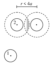
Figure 1: The “shielding” effect. If a third molecule is sufficiently close to molecule 2, then the surface area of molecule 2’s associated sphere (dashed) which is accessible to molecule 1’s center is reduced by a dome (grayed). For further discussion of this effect see Ref. hockey, .

Since we can only be certain that molecule 1 has maintained a constant velocity during time $t$, it makes sense to use the rest frame of molecule 1 in which to evaluate the probability that other molecules miss molecule 1. It will be convenient to imagine that the center of molecule 1 occupies a single point, say, the origin of our box. During time $t$ the associated sphere of molecule 2 sweeps out a piecewise cylindrical volume equal to $\pi(2a)^{2}|\mathbf{v}_{2}-\mathbf{v}_{1}|t$.endcap The probability that the origin is not in the swept-volume of 2’s associated sphere would appear to be

$$p_{2}=\frac{\bigl{[}L^{3}-\frac{4}{3}\pi(2a)^{3}(N-1)\bigr{]}-\sigma|\mathbf{v}_{2}-\mathbf{v}_{1}|t}{L^{3}-\frac{4}{3}\pi(2a)^{3}(N-1)}.$$ (15)

However, due to the previously mentioned shielding effect there is a reduced likelihood of molecule 2 colliding with molecule 1 since, at any given moment, only a fraction of the surface area of molecule 2’s associated sphere is available to make contact with molecule 1’s center. That fraction is explicitly computed in Ref. Chapman, and what follows is an exposition of their procedure. The probable number of molecular centers within a range $r$ to $r+dr$ of the center of any chosen molecule is $n4\pi r^{2}dr$.pair Note that for a spatially uniform gas this number is independent of the positions of other molecules. Two overlapping associated spheres whose centers are separated by a distance $2a<r<4a$ obstruct, on either sphere, a dome with lateral area $4\pi a(2a-r/2)$. Therefore, the probable area unavailable to a molecule is

$$\int_{2a}^{4a}n4\pi r^{2}dr\cdot 4\pi a(2a-r/2)=\frac{11}{3}\pi^{2}(2a)^{5}n.$$ (16)

The available fractional area of molecule 2’s associated sphere which can collide with molecule 1’s center is thus

$$\frac{4\pi(2a)^{2}-\frac{11}{3}\pi^{2}(2a)^{5}n}{4\pi(2a)^{2}}=1-\frac{11}{12}\pi(2a)^{3}n.$$ (17)

Expression (17) must multiply the swept-volume of molecule 2’s associated sphere. As a check, if expression (17) is zero then there is unit probability that the origin lies outside the swept-volume. The correct modification of expression (15) is therefore

$$p_{2} = \frac{\bigl{[}L^{3}-\frac{4}{3}\pi(2a)^{3}(N-1)\bigr{]}-\bigl{[}\sigma|\mathbf{v}_{2}-\mathbf{v}_{1}|t\bigr{]}\bigl{[}1-\frac{11}{12}\pi(2a)^{3}n\bigr{]}}{L^{3}-\frac{4}{3}\pi(2a)^{3}(N-1)}$$ (18)

$$= 1-\frac{\sigma n\chi|\mathbf{v}_{2}-\mathbf{v}_{1}|\ell/|\mathbf{v}_{1}|}{N},$$

where

$$\chi\equiv\frac{1-\frac{11}{12}\pi(2a)^{3}n}{1-\frac{4}{3}\pi(2a)^{3}(n-L^{-3})}=1+\frac{5}{12}\pi(2a)^{3}n+o(n^{2})+o(L^{-3}).$$ (19)

In a large-volume limit the correction of $o(L^{-3})$ is subleading and may be neglected. Moreover, we have neglected corrections imposed by the boundary. We see that effect (i) tends to increase the probability of collisions whereas effect (ii) tends to decrease it. Higher order corrections to $\chi$ are known.Chapman

A similar argument can be made concerning the probability $p_{3}$ that the swept-volume of molecule 3’s associated sphere does not contain the origin. We assume the probabilities $p_{2}$, $p_{3}$, etc. to be independent, essentially invoking the molecular chaos assumption. However this does not preclude the $N-1$ particles from interacting with each other during time $t$; their collisions will inevitably “kink” each other’s cylinders. The probability that none of the $N-1$ associated spheres hits molecule 1’s center during this time is given by the product of the individual probabilities:

$$p(\ell|\mathbf{v}_{1})=\prod_{i=2}^{N}p_{i}=\prod_{i=2}^{N}\biggl{[}1-\frac{\sigma n\chi|\mathbf{v}_{i}-\mathbf{v}_{1}|/|\mathbf{v}_{1}|}{N}\ell\biggr{]}.$$ (20)

In this product the values of $\mathbf{v}_{i}$ are obtained from the equilibrium velocity distribution. One way to estimate this product is to discretize the velocity distribution into a finite number of bins and assign to each $\mathbf{v}_{i}$ a particular value representative of a bin. In the $j$th bin there will be $Nf(\mathbf{v}_{j})d^{3}v_{j}$ particles. Thus,

$$p(\ell|\mathbf{v}_{1}) = \prod_{\text{bins}~{}j}\Biggl{[}1-\frac{\sigma n\chi|\mathbf{v}_{j}-\mathbf{v}_{1}|/|\mathbf{v}_{1}|}{N}\ell\Biggr{]}^{Nf(\mathbf{v}_{j})d^{3}v_{j}}$$ (21)

$$= \exp\sum_{j}-\sigma n\chi\ell\frac{|\mathbf{v}_{j}-\mathbf{v}_{1}|}{|\mathbf{v}_{1}|}f(\mathbf{v}_{j})d^{3}v_{j}$$

$$= \exp\biggl{[}-\frac{\sigma n\chi\ell}{|\mathbf{v}_{1}|}\int d^{3}v\,f(\mathbf{v})|\mathbf{v}-\mathbf{v}_{1}|\biggr{]}.$$

In the second step we took the limit of large $N$ (and large volume so as to keep the concentration fixed and small compared to 1) and in the third step the sum was generalized to a continuous integral over all possible velocities. The collision rate is found by comparing Eq. (21) with $p(t|\mathbf{v}_{1})=\exp(-r(v_{1})\ell/|\mathbf{v}_{1}|)$. We obtain the well-known formula

$$r(v_{1})=\sigma n\chi\int d^{3}v\,f(\mathbf{v})|\mathbf{v}-\mathbf{v}_{1}|.$$ (22)

As one might expect the probability of collision is high when the cross section is large, the gas is dense, or if the relative speed is large.Reifsrate The integral can be done by orienting the $z$-axis along $\mathbf{v}_{1}$ so that the magnitude of the relative velocity $\mathbf{v}-\mathbf{v}_{1}$ may be computed from the law of cosines as $\sqrt{v^{2}+v_{1}^{2}-2vv_{1}\cos\theta}$, where $\theta$ is the polar angle. Doing the angular and radial integrations in order produces

$$r(v_{1}) = \sigma n\chi\sqrt{\frac{2}{\pi}}\int_{0}^{\infty}dv\,v^{2}e^{-\tfrac{1}{2}v^{2}}\times\begin{cases}v+\frac{v_{1}^{2}}{3v}&v>v_{1}\,,\\ v_{1}+\frac{v^{2}}{3v_{1}}&v<v_{1}\,,\end{cases}$$ (23)

$$= \sigma n\chi\Biggl{[}\sqrt{\frac{2}{\pi}}\exp\biggl{(}-\frac{v_{1}^{2}}{2}\biggr{)}+\bigl{(}v_{1}+v_{1}^{-1}\Bigr{)}\text{erf}\biggl{(}\frac{v_{1}}{\sqrt{2}}\biggr{)}\Biggr{]}.$$

Here erf is the error function. The collision rate is finite as $v_{1}\to 0$, monotone increasing, and behaves asymptotically as $r(v_{1})/\sigma n\chi\sim v_{1}+o(1/v_{1})$. The fact that $r(v_{1})$ scales as $v_{1}$ for large speed is completely expected based on the fact that the majority of molecules have relatively low speeds compared to the very few molecules in the tail of the Maxwell distribution. For $v_{1}$ much larger than the characteristic speed set by the temperature it is as if all molecules except for molecule 1 are frozen in place. Then it is easy to see that the frequency of scattering events incurred by molecule 1 is directly proportional to its speed. Notice that the term in Eq. (23) which dominates the asymptotic behavior does indeed come from the $v_{1}>v$ domain of integration. More to the point, if we approximate the relative speed $|\mathbf{v}-\mathbf{v}_{1}|$ by just $v_{1}$ in Eq. (22), then the integral evaluates to $v_{1}$.

V Explicit results for the hard-sphere gas

The collision rate found in Eq. (23) may be averaged in the equilibrium velocity distribution to obtain the mean collision rate:

$$\omega=\left\langle r(v)\right\rangle=\frac{4}{\sqrt{\pi}}\sigma n\chi.$$ (24)

We may compare predictions for this rate with the numerical results of molecular dynamics simulations of a hard-sphere gas over a wide range of density. In Fig. 2 we plot Eq. (24) against data from Ref. Lue, . As expected, Eq. (24) deviates from the actual collision frequency when the density of the gas increases. The discrepancy is less than 10% for densities below $0.3(2a)^{-3}$.

Figure 2: Average collision frequency in the hard-sphere gas versus density. The frequency is given in units of $(kT/m)^{1/2}(2a)^{-1}$ and the density is measured in units of $(2a)^{-3}$. The solid line is the predicted rate $\omega$ from Eq. (24) using $\chi=1+\frac{5}{12}\pi(2a)^{3}n$, and the dashed line is the predicted rate with $\chi=1$. The dots are the reciprocal of the average time between collisions taken from Table I of Ref. Lue, . The density range shown is between 0, the extreme dilute limit, and 1, which is somewhat close to the limit of close packing of the spheres within the container. The fractional error between the predicted and simulated collision frequency grows with increasing density. It is less than 10% only for $n(2a)^{3}<0.3$.

The on-collision distribution in terms of speed, $f_{\textrm{coll}}(v)4\pi v^{2}dv$, is evidently independent of the molecular size and density of the gas. The mean speed is $(3+\pi)/(2\sqrt{\pi})\approx 1.7325$ and the most probable speed is found numerically to be $1.5769$. These may be contrasted with the corresponding values $\sqrt{8/\pi}\approx 1.5958$ and $\sqrt{2}\approx 1.4142$, respectively, for the Maxwell speed distribution, which are lower. The on-collision speed distribution results from multiplying the Maxwell speed distribution by the monotonically increasing function $r(v)/\omega$ which skews the distribution toward larger $v$. These two distributions are plotted in Fig. 3.

Figure 3: Different types of probability density functions for speeds. Speed is measured in units of $(kT/m)^{1/2}$ and each density function has the inverse unit. The dashed curve represents the Maxwellian probability density $4\pi v^{2}f(v)$ for randomly picking a molecule with speed $v$ from the gas. The solid curve represents the probability density $4\pi v^{2}f_{\textrm{coll}}(v)$ for finding a molecule with incoming speed $v$ when one member of a colliding pair is examined at random. This figure appears in Ref. Lue, .

The free path length distribution given in Eq. (13), when appropriately normalized, may be expressed in terms of a scaling function. That is,

$$\lambda_{\textrm{Maxwell}}P(\ell/\lambda_{\textrm{Maxwell}})=F(\ell/\lambda_{\textrm{Maxwell}}),$$ (25)

where

$$F(x)\equiv\frac{1}{\pi}\int_{0}^{\infty}\frac{dv}{v}\psi(v)^{2}\exp\biggl{[}-v^{2}-\frac{1}{\sqrt{2\pi}}v^{-2}\psi(v)x\biggr{]},~{}~{}~{}~{}\psi(v)\equiv ve^{-v^{2}}+(2v^{2}+1)\int_{0}^{v}e^{-t^{2}}dt.$$ (26)

The scaling function $F$ does not depend on any dimensionless parameters other than its argument which is the ratio of the free path length and the mean free path. In particular, $F$ is independent of the reduced density $n(2a)^{3}$. This striking density independence of the scaled free path length distribution was noticed in early molecular dynamics simulations of fluids.Alderletter

A plot of $\ln F$ is shown in Fig. 4 and it is contrasted with a plot of $-x$ in order to show the deviations from pure exponential behavior. The special result $F(x)=e^{-x}$ would only result if all molecules in the gas were stationary except for the one molecule executing a free path. This would correspond to a collision rate $r(v)\propto v$ for which the computation of Eq. (13) can be done explicitly and yields a simple exponential. To evaluate the long-distance behavior of $F(x)$ given by Eq. (26) one can use the method of steepest descent.steepest It turns out that $F(x)\sim e^{-x/\sqrt{2}}$. Further discussion of the distribution may be found in the original Refs. ViscoShort, ; ViscoLong, .

Figure 4: Logarithm of the scaling function for the free path length density. The solid curve is $\ln F(x)$. In the text it is shown that the distribution of free path lengths, $P(\ell)d\ell$, when parametrized in units of the mean free path as $x=\ell/\lambda_{\textrm{Maxwell}}$, is given by $F(x)dx$. For contrast the dashed curve is a straight line with negative unit slope. The disagreement between $\ln F(x)$ and $-x$ shows that the free path length density is not a simple decaying exponential. Its behavior simplifies somewhat for asymptotically large $x$: the dominant term is exponential and of the form $\ln F(x)\sim-x/\sqrt{2}$, although this slope is only apparent for $x\sim o(100)$ and higher.ViscoShort ; ViscoLong

In Fig. 5 we plot the scaling function $F$ and data obtained from Einwohner and Alder’s early molecular dynamics simulation of the hard-sphere fluid at three different densities. Even for very dense fluids the agreement is excellent.mistake

Figure 5: Scaling for the distribution of free path lengths. The solid curve is $F(x)$. In the text it is shown that the distribution of free path lengths, $P(\ell)d\ell$, when parametrized in units of the mean free path as $x=\ell/\lambda_{\textrm{Maxwell}}$, is given by $F(x)dx$. The data is obtained from Table VIII of Ref. Einwohner, . The numerical simulations were done at three densities: $n(2a)^{3}\approx 0.47$ (triangles), $0.71$ (crosses), and $0.88$ (circles). This figure appears in Ref. Alderletter, but with a subtle difference.mistake The inset shows the difference between the theoretical curve and simulated data.

*

Appendix A The meaning of $\chi$

In Appendix A of Ref. Einwohner, Einwohner and Alder prove that the mean collision rate per molecule $\omega(n)$ in a hard-sphere fluid with number density $n$ is $\omega(n)=\omega(n\to 0)\chi(n)$. Here $\omega(n\to 0)=\frac{4}{\sqrt{\pi}}\sigma n\sqrt{\frac{kT}{m}}$ is the collision frequency in the limit of infinite dilution and $\chi(n)$ is directly related to the probability that, when given a sphere, there will be any other one located at a center-to-center distance of $2a$. We discuss the salient points of their proof.

Suppose that the $N$ spheres experience a total of $M$ collisions during a time $t_{0}$ which is much longer than the average time between collisions. The total collision rate may be written as a time average,

$$N\omega=M/t_{0}=\frac{1}{t_{0}}\int_{0}^{t_{0}}dt\,\sum_{k=1}^{M}\delta(t-t_{k}),$$ (27)

where $\{t_{k}\}$ are the times at which the collisions occur. Imagine that one knows the trajectories $\mathbf{r}_{i}(t)$ of all $N$ spheres parametrized by the time $t$. Then the sum of delta functions in time may be reexpressed as a sum of delta functions involving the trajectories,

$$\sum_{k=1}^{M}\delta(t-t_{k})=\sum_{i=2}^{N}\sum_{j=1}^{i-1}\delta(\mathbf{r}_{ij}(t)^{2}-4a^{2})\theta(-\mathbf{r}_{ij}\cdot\mathbf{v}_{ij})|2\mathbf{r}_{ij}\cdot\mathbf{v}_{ij}|.$$ (28)

We use the notation $\mathbf{r}_{ij}\equiv\mathbf{r}_{i}-\mathbf{r}_{j}$ and a similar one for the relative velocity. The expression in terms of the particles’ phase space coordinates is more complicated since a collision requires that two conditions be met: that the sphere centers are one diameter apart and that the relative velocity of the spheres must make an obtuse angle with the separation vector, the vector pointing from the center of sphere $j$ to the center of sphere $i$. The latter condition is necessary to pick out only those events in phase space where spheres are just about to collide and to avoid those events where spheres depart or pass parallel without touching; it has been incorporated using the unit step function $\theta$ which equals 1 for positive argument and 0 otherwise. Note that a Jacobian factor involving the relative velocity is required by the change of variables. The equality of time and ensemble averages is now invoked:

$$\frac{1}{t_{0}}\int_{0}^{t_{0}}O(t)dt=\frac{\int e^{-H/kT}O(\{\mathbf{r}_{i}(t)\},\{\mathbf{v}_{i}(t)\})\,d\mathbf{r}_{1}\dotsb d\mathbf{r}_{N}\,d\mathbf{v}_{1}\dotsb d\mathbf{v}_{N}}{\int e^{-H/kT}d\mathbf{r}_{1}\dotsb d\mathbf{r}_{N}\,d\mathbf{v}_{1}\dotsb d\mathbf{v}_{N}},$$ (29)

where $H=\tfrac{1}{2}m\sum_{i=1}^{N}\mathbf{v}_{i}^{2}+\Phi(\mathbf{r}_{1},\dotsc,\mathbf{r}_{N})$ is the classical energy of the system. The potential energy is a sum of two-body terms that only depends on the separations between particles: $\Phi=\sum_{i<j}\phi(|\mathbf{r}_{ij}|)$, where $\phi$ is infinite if $|\mathbf{r}_{ij}|$ is strictly less than $2a$ and zero otherwise. Since the Boltzmann factor factorizes into a product of kinetic and potential terms the velocity integrals can be done exactly. The delta function then collapses two of the position integrals. One obtains

$$\omega=\frac{4}{\sqrt{\pi}}\sqrt{\frac{kT}{m}}\,\pi(2a)^{2}\,\frac{N-1}{V}\,\underbrace{\frac{V^{2}\int d\mathbf{r}_{3}\dotsb d\mathbf{r}_{N}\,e^{-\Phi(|\mathbf{r}_{12}|=2a,|\mathbf{r}_{13}|,\dotsc)/kT}}{\int d\mathbf{r}_{1}\dotsb d\mathbf{r}_{N}\,e^{-\Phi(|\mathbf{r}_{12}|,|\mathbf{r}_{13}|,\dotsc)/kT}}}_{\chi}.$$ (30)

For a uniform fluid $\chi$ is a function of the reduced density $n(2a)^{3}$. If we assume that the molecular chaos approximation holds even when the gas is dense so that the density of molecular centers in the immediate neighborhood of a molecule is not correlated to the velocity of that molecule, then we would also expect that the collision rate $r(v)$ experienced by any molecule moving with speed $v$ is directly proportional to the same factor $\chi$ derived above. See the discussion in Ref. Chapman, . In particular, $\chi$ does not depend on $v$.

- (1) See, for example, Frederick Reif, Fundamentals of Statistical and Thermal Physics (Waveland Press, Long Grove, IL, 2008), pp. 463–471.
- (2) Sydney Chapman and T. G. Cowling, The Mathematical Theory of Non-Uniform Gases (Cambridge University Press, New York, 1970), pp. 58–96, 297–300.
- (3) The densest packing of spheres results in a periodic array of spheres that occupy approximately 74% of the total available volume. This corresponds to a number density of .
- (4) Protagoris Cutchis, H. van Beijeren, J. R. Dorfman, and E. A. Mason, “Enskog and van der Waals play hockey,” Am. J. Phys. 45, 970–977. These authors focus on a hard-disk fluid in two dimensions but mention the generalizations to hard spheres in three dimensions.
- (5) Explicitly, , where .
- (6) T. Einwohner and B. J. Alder, “Molecular Dynamics. VI. Free-Path Distributions and Collision Rates for Hard-Sphere and Square-Well Molecules.” J. Chem. Phys. 49, 1458–1473 (1968).
- (7) J. H. Jeans, The Dynamical Theory of Gases (Cambridge University Press, London, 1904), pp. 229–241.
- (8) In passing we remark that if the collision rate were independent of speed then all three definitions of the mean free path would give identical values. For instance, in Morton Masius, “On the Relation of Two Mean Free Paths,” Am. J. Phys. 5, 260–262, it is explicitly demonstrated how Tait’s definition yields the same value as Maxwell’s definition of the mean free path.
- (9) Paolo Visco, Frédéric van Wijland, and Emmanuel Trizac, “Non-Poissonian Statistics in a Low-Density Fluid,” J. Phys. Chem. B 112, 5412–5415 (2008).
- (10) Paolo Visco, Frédéric van Wijland, and Emmanuel Trizac, “Collisional statistics of the hard-sphere gas,” Phys. Rev. E 77, 041117 (2008).
- (11) L. Lue, “Collision statistics, thermodynamics, and transport coefficients of hard hyperspheres in three, four, and five dimensions,” J. Chem. Phys. 122, 044513 (2005).
- (12) This is a proper probability, not a density. Note that . It may be obtained by imagining that the finite time is discretized into equal intervals . Then the probability to not undergo a collision in steps is . In the limit that , becomes exponential.
- (13) A similar reasoning is used to obtain the molecular speed distribution of a hot gas effusing through a small hole in an oven. Recall that the Maxwell speed distribution is weighted by an additional factor of the speed reflecting the fact that faster molecules bombard the hole with greater frequency than slower molecules — that relative frequency is the ratio of their speeds.
- (14) This is an approximation based on the observation that the number of overlapping associated spheres in a dilute gas is small compared to the total number of spheres. In order to correct for the possibility of overlap we note that the probable number of molecules close enough to any given molecule for their associated spheres to overlap is proportional to . Therefore, the probable excluded volume on any molecule scales as . And there are order molecules. Thus, the overlap correction to the naive inhabitable volume estimate appears at in the factor .
- (15) It is unnecessary to include contributions to the volume from the hemispherical endcaps. This is accounted for when we reduce the amount of inhabitable volume of molecule 1 due to the volumes of the other molecules.
- (16) Actually, the right expression is , where is the radial distribution function for the hard-sphere gas. Expanding in the density, . The lowest order term, 1, is sufficient to calculate to accuracy.
- (17) In Ref. Reif, a remark given on p. 470 summarizes a rigorous traditional derivation of the collision rate that is more general than the one given in this article. Reif’s expression involves an additional integration over all solid angle of a differential scattering cross section which can be computed for an arbitrary interaction potential between molecules.
- (18) B. J. Alder and T. Einwohner, “Free-Path Distribution for Hard Spheres.” J. Chem. Phys. 43, 3399–3400 (1965).
- (19) For very large the main contribution to the integral comes from an environment of wherein the function , which multiplies the factor in the exponent of the integrand, goes through a maximum. This happens as . Therefore, the dominant asymptotic behavior of the integral is of the form , where .
- (20) In Ref. Einwohner, the authors actually formulate the scaled free path length distribution without the additional factor of since they incorrectly assumed that the probability to find a molecule with a given speed in a collision was given by the Maxwell speed distribution. In our notation they found . Somewhat fortuitously, the error incurred by using the wrong distribution makes a very small adjustment to the shape of the scaling function. The absolute value of the difference between and is no greater than about 0.07 and this occurs for small values of the argument. Such discrepancy is noticeable in Fig. 1 of Ref. Alderletter, . Note that the correct scaling function predicts which matches the data better at very small free path length than is reported in that letter.