A Joint Model Of X-ray And Infrared Backgrounds. II. Compton-Thick AGN Abundance

Abstract

We estimate the abundance of Compton-thick (CT) active galactic nuclei (AGN) based on our joint model of X-ray and infrared backgrounds. At $L_{\rm rest2-10keV}$ $>$ 10⁴² erg/s, the CT AGN density predicted by our model is a few $\times$10^-4 Mpc^-3 from $z$=0 up to $z$=3. CT AGN with higher luminosity cuts ($>$ 10⁴³, 10⁴⁴ & 10⁴⁵ erg/s) peak at higher $z$ and show a rapid increase in the number density from $z$=0 to $z$$\sim$2-3. The CT to all AGN ratio appears to be low (2-5%) at $f_{\rm 2-10keV}$ $>$ 10^-15 erg/s/cm² but rises rapidly toward fainter flux levels. The CT AGN account for $\sim$ 38% of the total accreted SMBH mass and contribute $\sim$ 25% of the cosmic X-ray background spectrum at 20 keV. Our model predicts that the majority (90%) of luminous and bright CT AGN ($L_{\rm rest2-10keV}$ $>$ 10⁴⁴ erg/s or $f_{\rm 2-10keV}$ $>$ 10^-15 erg/s/cm²) have detectable hot dust 5-10 $\mu$m emission which we associate with a dusty torus. The fraction drops for fainter objects, to around 30% at $L_{\rm rest2-10keV}$ $>$ 10⁴² erg/s or $f_{\rm 2-10keV}$ $>$ 10^-17 erg/s/cm². Our model confirms that heavily-obscured AGN ($N_{\rm HI}$ $>$ 10²³ cm^-2) can be separated from unobscured and mildly-obscured ones ($N_{\rm HI}$ $<$ 10²³ cm^-2) in the plane of observed-frame X-ray hardness vs. mid-IR/X-ray ratio.

1. Introduction

Active galactic nuclei (AGN) with Compton-thick (CT) nuclear obscuration ($N_{\rm HI}$ $>$ 1.5$\times$10²⁴ cm^-2) are a crucial piece in the quest for a complete census of the AGN population. While Chandra and XMM-Newton have revealed a large population of AGN up to $z$$\sim$5 and demonstrated unambiguously the dominance of supermassive black-hole (SMBH) accretion in the obscured phase (Mainieri et al., 2002; Perola et al., 2004; Hasinger et al., 2005; Barger et al., 2005), the necessity of having a high SNR X-ray spectrum including detection above and below rest-frame energies of 10 keV, largely limits the detectability to reveal the presence of CT AGN in deep surveys (Tozzi et al., 2006; Georgantopoulos et al., 2009). However, there are several compelling reasons to suspect an abundant distant CT AGN population: (1) in the local universe the CT AGN comprise roughly 50% of the optically-selected AGN sample (Risaliti et al., 1999; Guainazzi et al., 2005); given the dusty high-$z$ universe, the distant CT AGN may be more abundant. (2) Cosmic X-ray background (CXB) population models invoke luminosity functions of AGN with different HI columns to fit the X-ray survey data (Comastri et al., 1995; Gilli et al., 2007; Treister et al., 2009a), which requires a large number of CT AGN to re-produce the CXB spectrum at its peak (20-30 keV) ; this general conclusion is largely independent of detailed assumptions in the model. (3) The multi-wavelength techniques that combine the X-ray data with optical/IR photometry offer powerful ways to identify CT candidates, and indicate an increasing spatial density of CT AGN with redshift (Alexander et al., 2008; Daddi et al., 2007; Fiore et al., 2009; Luo et al., 2011; Treister et al., 2009b).

In Shi et al. (2013) (hereafter Paper I), we presented a joint population model of X-ray and infrared backgrounds that fits the survey data in the 0.5-60 keV and 24-1200 $\mu$m bands, with the goal of studying the cosmic evolution of AGN and dusty starbursts. We discuss here the CT AGN abundance derived from this model. In contrast to CXB models that only fit X-ray data primarily at energies below 10 keV, our approach is fundamentally different. CXB models usually use 0.1-10 keV data to fit the Compton-thin AGN counts, extrapolate the result to 20-30 keV and then subtract this from the CXB spectrum to derive the abundance of CT AGN. Our model constrains the Compton-thin AGN from 0.5-10 keV data and starburst galaxies from far-IR data, and compares the 24 $\mu$m from these populations to the IR background and known distributions of 24 $\mu$m-detected sources. The residual of the 24$\mu$m emission after subtracting the contributions from Compton-thin and starburst galaxies is assumed to be from Compton-thick AGN. As a result, our model uses more observational information to constrain the CT AGN fractions as a function of luminosity and redshift, including both number counts and redshift distributions at 24 $\mu$m. In our model, we allow the redshift evolution of the CT AGN to be a free parameter, while the CXB models typically assume no evolution, fixed evolution or an evolution as the same as the Compton-thin AGN.

The spectral energy distribution (SED) of individual sources is crucial to any population model, but our joint model and the CXB models depend on different parts of the SED. The CXB model is sensitive to the X-ray SED above 10 keV (e.g. Gilli et al., 2007; Treister et al., 2009a), while ours relies on the 24$\mu$m/2-10keV ratio of the SMBH SED but also the star-forming IR SED. As a result, we ran four variants of the model to incorporate the SED uncertainties, including the reference one, the one with X-ray to IR ratio of the SMBH SED 3-$\sigma$ (0.2 dex) above the average ratio, the one with X-ray to IR ratio of the SMBH SED 3-$\sigma$ (0.2 dex) below the average ratio and the one assuming strong redshift evolution in the star-forming SED (for details, see Paper I). Overall, our model provides a new way to constrain the CT AGN abundance using substantially more information from more diverse deep survey data. Paper I presented the detailed model construction and three basic outputs including the total IR luminosity function, the SMBH energy fraction in the IR band and HI column density distributions as a function of X-ray luminosity and redshift.

In this paper we discuss the predicted CT AGN abundance and compare it to a large collection of empirical constraints. In § 2, we show the spatial number density of CT AGN. We present the type-2 and CT AGN fraction as a function of X-ray fluxes in § 3. The contribution of CT AGN to the SMBH accretion and CXB spectrum is shown in § 4. Discussions and conclusions are presented in § 5 and § 6, respectively.

2. The Comoving Number Density Of Compton-Thick AGN

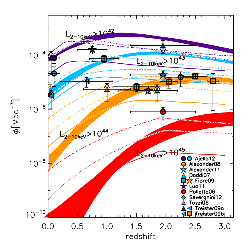
Figure 1.— Comoving number density of CT AGN above different intrinsic 2-10 keV luminosities as a function of redshift. The filled areas represent the predictions of our model in each of four luminosity bins. The width of the curves reflect the uncertainties of the predictions. The solid, dotted and dotted-dashed lines are the predictions by the cosmic X-ray background models of Treister et al. (2009a), Gilli et al. (2007) and Draper & Ballantyne (2010), respectively. All symbols represent the observations. A symbol is plotted with a filled core plus a black envelope. For all filled areas, lines and symbol cores, purple: $L_{\rm 2-10keV}$ $>$ 10⁴² erg/s, cyan: $L_{\rm 2-10keV}$ $>$ 10⁴³ erg/s, orange: $L_{\rm 2-10keV}$ $>$ 10⁴⁴ erg/s, and red: $L_{\rm 2-10keV}$ $>$ 10⁴⁵ erg/s.

Figure 1 shows the predicted comoving number density of CT AGN above different intrinsic rest-frame 2-10 keV luminosity limits as a function of redshift (filled areas with different colors). Symbols with the same color are the empirical estimates from the literature above the same limits. Among different variants of our model, as reflected by the vertical width of the filled area in the figure, the predicted number density varies from a factor of 2 for low luminosity objects ($>$ 10⁴² erg/s) up to a factor of 5 for luminous ones ($>$ 10⁴⁵ erg/s). For CT AGN with intrinsic $L_{\rm rest2-10keV}$ $>$ 10⁴² erg/s, our model predicts the density to peak at a few $\times$10^-4 Mpc^-3 around $z$ $\sim$ 1-1.5, declining slowly toward both higher and lower redshifts. The local densities as measured by Treister et al. (2009a) and Ajello et al. (2012) are consistent with our predictions. The estimate at $z$$\sim$0.7 by Luo et al. (2011) is only a factor of 2 lower than our prediction. They performed a Monte-Carlo simulation to estimate the CT AGN fraction in a sample of IR-excess sources defined as having excess IR emission relative to the UV-based star-forming emission (log(SFR_IR+UV/SFR_UV,corr) $>$ 0.5) (e.g. Daddi et al., 2007). The stacked X-ray spectrum of these sources shows evidence for heavy extinction. However, due to the lack of CT signatures in individual galaxies, this statistical approach still suffers from large uncertainties.

The more luminous CT AGN at $L_{\rm 2-10keV}$ $>$ 10⁴³ erg/s show a different trend, with a faster evolution starting at $z$=0 and a higher peak redshift. The predicted local density is consistent with empirical estimate by Treister et al. (2009a) and Severgnini et al. (2012) but three times lower than that by Ajello et al. (2012) yet within the uncertainty. The work by Treister et al. (2009a) only includes the transmission AGN, thus underestimating the total population if reflection-dominated CT AGN are abundant. Beyond the local universe, the density around $z$=0.7 by Treister et al. (2009b) is 3 times lower than the prediction of our model, while other high-z studies by Fiore et al. (2009), Daddi et al. (2007) and Alexander et al. (2011) give results consistent with the model. Among them, Daddi et al. (2007) gives a solid upper-limit, as they assume CT nature for all their IR-excess objects (log(SFR_IR+UV/SFR_UV,corr) $>$ 0.5), while Alexander et al. (2011) derived a solid lower-limit by only counting sources that satisfy the BzK selection detected in the X-ray.

At $L_{\rm 2-10keV}$ $>$ 10⁴⁴ erg/s, the comoving density of the CT AGN shows a rapid rise until $z$$\sim$2 and almost a flat trend up to $z$=3. The model’s prediction is more or less consistent with observations (Alexander et al., 2008; Fiore et al., 2009; Treister et al., 2009b) except for one data point around $z$$\approx$0.9 but within the uncertainty (Tozzi et al., 2006). Tozzi et al. (2006) analysed the X-ray spectra of sources in the 1Ms CDF-S and identified 14 CT AGNs, possibly missing the X-ray-undetected CT AGNs. At $L_{\rm 2-10keV}$ $>$ 10⁴⁵ erg/s, the CT AGN show a rapid evolution in the model, with two orders of magnitude increase in density from $z$=0 up to $z$=3. Model prediction around $z$$\sim$2 is lower than the estimate by Polletta et al. (2006). Although only X-ray detected sources are accounted for this measurement (Treister et al., 2009a), the low number of objects caution a large uncertainty associated with the measurement.

The predicted CT AGN number density of our model is generally similar to predictions by the CXB model of Gilli et al. (2007) (dotted lines in Figure 1) but ours peaks at higher redshift. The model of Gilli et al. (2007) assumed all X-ray sources detected at 0.5-2 and 2-10 keV to be Compton-thin and derived their distributions as a function of redshift, luminosity and HI columns. After subtracting the contribution of these Compton-thin sources from the CXB spectrum, the residual is not zero, thus implying the existence of CT AGN. By assuming the same redshift evolution for CT AGN as for obscured Compton-thin AGN, the amount of CT AGN is derived by matching to the CXB spectrum. At a given redshift and limiting X-ray luminosity, their result does not deviate from ours significantly. A significant difference however between the two models is that they predict a lower redshift for the peak of the CT AGN number density. For $L_{\rm 2-10keV}$ $>$ 10⁴² erg/s, our peak redshift is $z$$\sim$1-1.5 compared to theirs around $z\sim$0.7. A difference of $\Delta$$z$=0.5-1 in the peak redshift is also found for the number density of CT AGN at $L_{\rm 2-10keV}$ $>$ 10^43,44,45 erg/s.

The CXB model of Treister et al. (2009a) (solid lines in Figure 1) predicts lower CT AGN number densities than ours. At $L_{\rm 2-10keV}$ $>$ 10⁴² erg/s, our predicted CT density is 5-10 times higher than theirs across the whole redshift range. At higher luminosities ($>$ 10^43,44,45 erg/s), their predictions are similar to ours up to their turn-over redshift but lower by 5-10 at higher redshifts as our predicted density rises faster. This is not surprising, since Treister et al hold the CT fraction in obscured AGN constant at the local value seen in the INTEGRAL and Swift data, allowing for no redshift evolution. In contrast, our model requires more CT AGN at higher redshifts to satisfy the various sets of observations (see Paper I). As shown in the next section, our model has no problem in reproducing the CT AGN fraction as observed by INTEGRAL and Swift.

In the CXB model of Draper & Ballantyne (2010) (dotted-dashed lines in Figure 1), low luminosity CT AGN ($>$ 10⁴² erg/s and $>$ 10⁴³ erg/s) have comparable number densities to those predicted from our models at low redshift, but are noticeably lower than ours at high $z$. The opposite seems to be the case for the high luminosity CT AGN, where two models make similar predictions at high redshift, but differ at low redshift where the Draper & Ballantyne (2010) models predict more CT AGN than do our models. These differences reflect the weaker dependence of their models on luminosity and redshift (Draper & Ballantyne, 2010, 2009).

3. The Type-2 and CT AGN Fraction

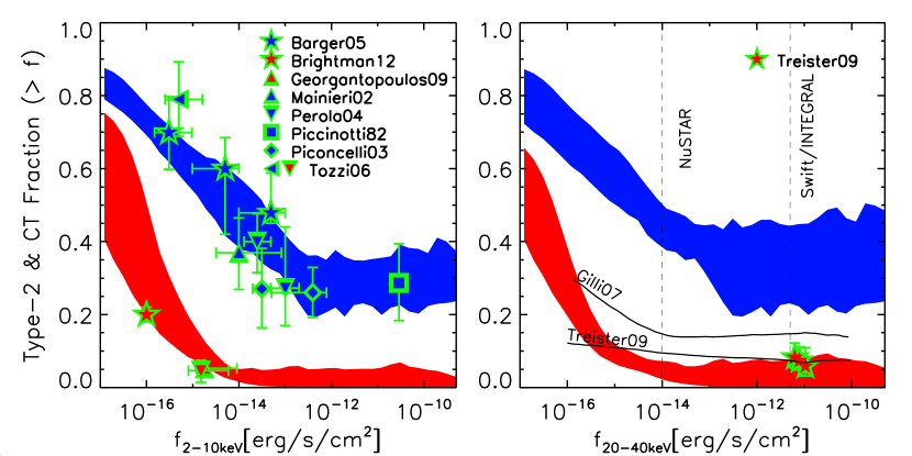
Figure 2.— Fraction of type-2 (upper band) and CT AGN (lower band) in all AGN as a function of 2-10 kev (left panel) and 20-40 keV (right panel) fluxes. The filled areas are our model’s predictions with the vertical width reflecting the uncertainty. The empirical estimates from the literature are indicated by symbols that are plotted with filled cores plus green outlines. For all symbol cores and filled areas, blue stands for type-2 AGN fraction (upper band) while red is for the CT AGN fraction (lower band). In the right panel, two solid lines are the CT AGN fractions predicted by models of Gilli et al. (2007) and Treister et al. (2009a). Dashed lines give the typical survey limits of NuSTAR, Swift and INTEGRAL.

Figure 2 plots the fractions of AGN that are type-2 ($N_{\rm HI}$ $>$ 10²² cm^-2) and Compton thick at different 2-10 keV and 20-40 keV fluxes. The two fractions show similar behaviors, i.e., a flat trend at bright fluxes along with a rapid rise toward fainter ends. Constant type-2 fractions of 30$\pm$10% and 35$\pm$10% are found at 2-10 keV and 20-40 keV above fluxes of 10^-13 erg/s/cm², respectively, while the CT AGN fractions remain around 3$\pm$3% and 4$\pm$3% at 2-10 keV and 20-40 keV above fluxes of 10^-15 erg/s/cm^-2, respectively. In Paper I, our model predicts a rapid redshift evolution of the type-2 and CT AGN fraction at given intrinsic X-ray luminosities, making the two fractions increase with decreasing fluxes, which combined with further obscuration to CT/type-2 objects results in a flat trend at bright fluxes but a rapid rise toward lower fluxes.

As shown in the figure, the predicted type-2 AGN fractions are consistent with empirical constraints as compiled in the work of Gilli et al. (2007) including Barger et al. (2005), Mainieri et al. (2002), Perola et al. (2004), Piccinotti et al. (1982), Piconcelli et al. (2003), and Tozzi et al. (2006). All these studies identified the type-2 in X-ray flux limited samples through X-ray spectral analysis. For the CT AGN fraction as a function of the 2-10 keV flux, we compared our predictions to empirical estimates based on studies of three X-ray flux limited samples (Tozzi et al., 2006; Georgantopoulos et al., 2009; Brightman & Ueda, 2012) that are constructed from Chandra 1 Ms, 2Ms and 4Ms survey data, respectively. The first two identified CT AGN through X-ray spectral analysis and derived CT fractions of 5% down to $f_{\rm 2-10keV}$=10^-15 erg/s/cm², consistent with the predictions of our model. The majority of these objects are CT AGN whose transmitted light dominates over the reflected radiation in X-ray. Brightman & Ueda (2012) carried out X-ray spectral analysis of 449 X-ray sources down to a flux 10 times lower ($f_{\rm 2-10keV}$=10^-16 erg/s/cm²), with average photon counts 3-5 times smaller than the other two studies. After corrections for these two effects, they argued for 20$\pm$2% CT AGN fraction, lower than our model’s prediction but within the uncertainty. At 20-40 keV, our result is consistent with the CT fraction as identified in Swift/INTEGRAL data (Treister et al., 2009a) in which all CT AGN are identified as transmission sources. The recently launched NuSTAR mission should offer strong constraints on the CT AGN fraction down to 10^-14 erg/s/cm².

As already discussed in the previous section, our model predicts roughly the same CT AGN abundance as the model of Gilli et al. (2007) but our predicted CT AGN number density peaks at higher redshift. This is also reflected in Figure 2 (right panel) where our CT fraction is lower than theirs above 10^-15 erg/s/cm² but exceeds theirs at fainter flux levels. Compared to the model of Treister et al. (2009a), our model predicts more abundant CT AGN at high $z$, resulting in a similar CT fraction above 10^-15 erg/s/cm² but a significantly higher fraction in our model at fainter fluxes.

4. The Contribution Of CT AGN To SMBH Growth And CXB

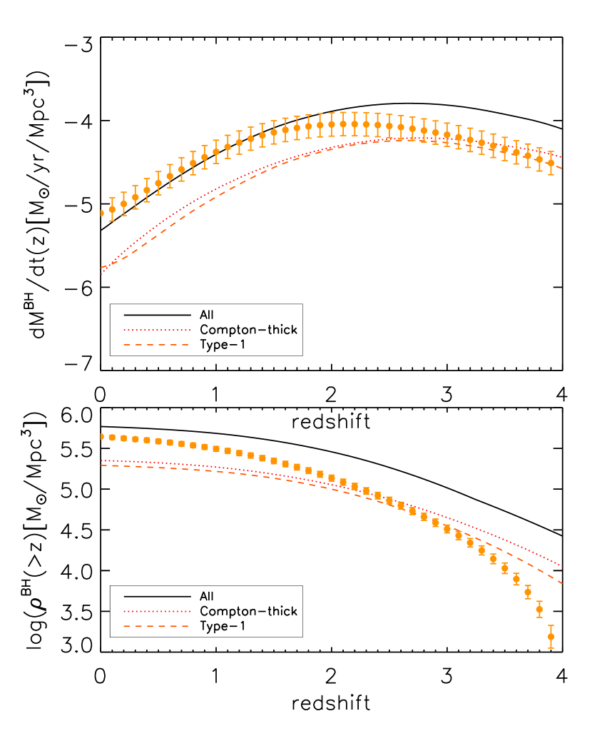
Figure 3.— Comoving SMBH accretion rate (upper panel) and total accreted SMBH mass density (lower panel) for all AGN (solid lines), type-1 (dashed lines) and Compton-thick (dotted lines) predicted from our model. Each line is the median value of the predictions from four model variants (see Paper I), while the uncertainty of the predictions among model variants is around 50%. Symbols are from Hopkins et al. (2007). Our predicted accretion rates seem to match those presented in Hopkins et al. (2007) up to $z$=2, but exceed theirs at higher redshifts, while the discrepancy in the cumulative accreted SMBH mass across the redshift is caused by that above $z$=2.

An SMBH grows through accretion, and the accretion disk is responsible for the optical through X-ray emission. By introducing the radiative efficiency $\epsilon_{r}$, the observed SMBH luminosity and accretion rate are related by:

$$L_{\rm ox}^{{}^{\prime}}=\epsilon_{r}\dot{M}_{\rm BH}c^{2}$$ (1)

where $L_{\rm ox}^{{}^{\prime}}$ is the luminosity integrated from the optical to the X-ray (1 $\mu$m to 200 keV), $\epsilon_{r}$ is the mass to energy conversion rate, $\dot{M}_{\rm BH}$ is SMBH mass accretion rate and $c$ is the speed of light. As constructed in Paper I, our quasar SED invokes the luminosity-dependent optical to X-ray ratio, and thus the correction from 2-10 keV to the luminosity from 1 $\mu$m to 200 keV is luminosity dependent with an average value around a factor of 30. Figure 3 shows the comoving SMBH accretion rate (upper panel) and cumulative accreted SMBH mass above a given redshift (lower panel). Our predicted accretion rates seem to match those presented in Hopkins et al. (2007) up to $z$=2, but exceed theirs at higher redshifts, while the discrepancy in the cumulative accreted SMBH mass across the redshift is caused by that above $z$=2. We believe the discrepancy to be related to the large uncertainties in deriving the obscured AGN LFs at these redshifts. The derived local SMBH mass density is (5.8$\pm$1.0)$\times$10⁵ M_⊙ Mpc^-3 given $\epsilon_{r}$=0.1. This number is quite consistent with those derived from local bulge mass functions through the bulge/BH-mass relationship, (2.9$\pm$0.5)$\times$10⁵ M_⊙ Mpc^-3 (Yu & Tremaine, 2002), (4.2$\pm$1.1)$\times$10⁵ M_⊙ Mpc^-3 (Shankar et al., 2004) and $4.6^{+1.9}_{-1.4}$$\times$10⁵ M_⊙ Mpc^-3 (Marconi et al., 2004). Our model further predicts that only 33% of local SMBH mass is accreted in the type-1 phase while the CT accretion contributes as much as 38% to the local SMBH mass density.

Figure 4 shows our prediction for the CXB spectrum at 1-200 keV as compared to observations. Our model predicts a peak around 20 keV. Below 20 keV, our prediction matches the results of RXTE/PCA (Revnivtsev et al., 2003) and ASCA/SIS (Gendreau et al., 1995), but is about 20% lower than those of Swift/XRT (Moretti et al., 2009) and INTEGRAL/JEM-X (Churazov et al., 2007). At 20-100 keV, the model is systematically lower by 20-30% than the observations (Gruber et al., 1999; Ajello et al., 2008; Türler et al., 2010). We do not know exactly what causes the discrepancy but noticed that the model cannot re-produce the local 15-55 keV counts of Ajello et al. (2012) and the CXB spectrum above 20 keV at the same time. If the model fits the Ajello et al. (2012) counts, it under-produces the CXB spectrum above 20 keV. On the other hand, if the model is forced to fit the CXB spectrum, it would over-predict counts of Ajello et al. (2012). As noted in Ajello et al. (2012), previous CXB models have a similar problem, including Gilli et al. (2007), Treister et al. (2009a) and Draper & Ballantyne (2010), where they fit the CXB spectrum well but over-predict local 15-55 keV counts. A key observational input for the CXB models to fit both Ajello et al. (2008) counts and CXB spectrum above 20 keV is the rest-frame SED at energies above 20 keV which is still not well constrained given limited observations. But certainly we cannot exclude the possibility that our model has limitations in reproducing the CXB spectrum above 20 keV as it fits so many data points over a very large range of the frequency (X-ray and IR/submm) to minimize $\chi^{2}$.

As shown in the figure, type-1 AGN dominate the CXB below 5 keV, above which the type-2 are responsible for the majority of CXB emission. The CT AGN contribution rises quickly from low energy and peaks around $\sim$25% at 20 keV.

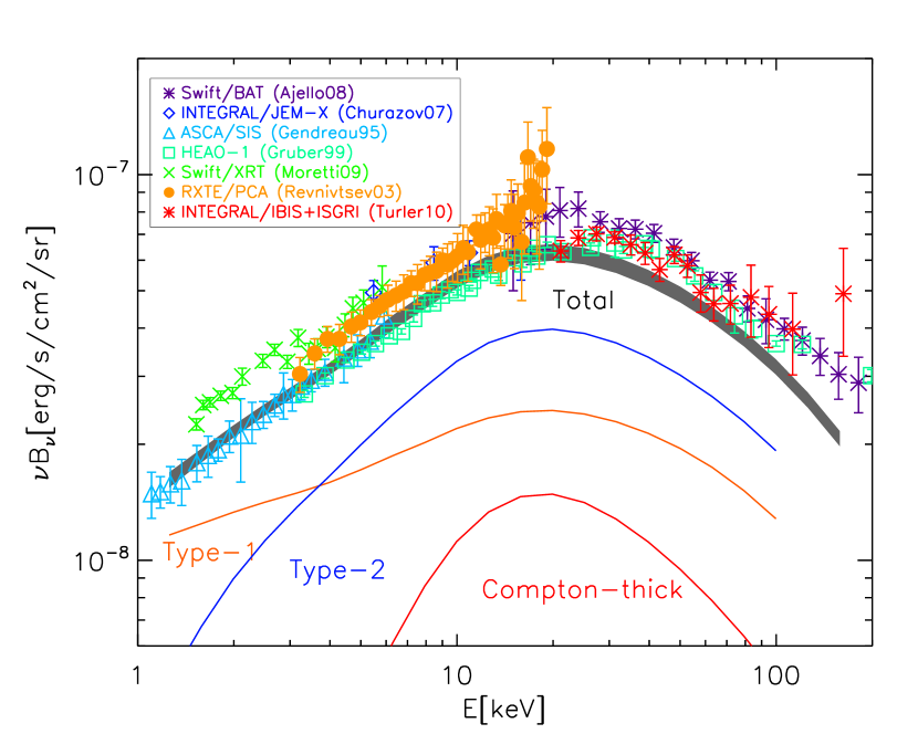
Figure 4.— The cosmic X-ray background spectrum from our model compared to the observations from the literature (all symbols). The grey curve is the prediction from our model, with the thickness of the curve representing the uncertainty in the model as a function of energy. Colored lines represent the median values of predictions by four model variants (see Paper I) for type-1 (orange), type-2 (blue) and Compton-thick (red) AGN as a function of energy. References: Ajello08 – Ajello et al. (2008); Churazov07 – Churazov et al. (2007); Gendreau95 – Gendreau et al. (1995); Gruber99 – Gruber et al. (1999); Moretti09 – Moretti et al. (2009); Revnivtsev03 – Revnivtsev et al. (2003); Turler10 – Türler et al. (2010).

5. Discussion

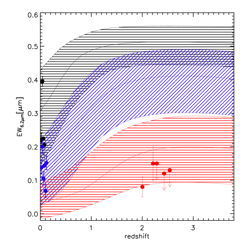
Figure 5.— Predicted median EW_6.2μmPAH and 20-80% probability range of CT AGN in three intrinsic X-ray luminosity ranges. Symbols are observations of low-z (Risaliti et al., 1999) and high-z (Alexander et al., 2008) CT AGN. For all shaded area and symbols, black: $L_{\rm 2-10keV}$=10⁴²-10⁴³ erg/s, blue: $L_{\rm 2-10keV}$= 10⁴³-10⁴⁴ erg/s and red: $L_{\rm 2-10keV}$ $>$ 10⁴⁴ erg/s. Note that in our model, pure star formation has a EW of 0.6 $\mu$m; any value below that is due to contributions from AGN emission.

Our model predicts an abundant CT AGN population especially at high-$z$. By comparing Figure 1 to the type-1 unobscured AGN number density as measured by Hasinger et al. (2005), our predicted CT AGN density is 3-5 times higher at $L_{\rm 2-10keV}$ $>$ 10⁴² erg/s. At $L_{\rm 2-10keV}$ $>$ 10⁴⁴ erg/s, the predicted CT AGN density is still comparable to their type-1 AGN around $z\sim$ 2. As shown in Paper I, our model predicts an increasing CT AGN fraction with redshift, resulting in a larger CT AGN population at high-$z$ as compared to the predictions of Gilli et al. (2007) and Treister et al. (2009a). The large CT AGN fraction around $z$ $\sim$ 2 may be consistent with observational evidence for high gas fractions and associated high SFRs of $z$$\sim$ 2 galaxies (Tacconi et al., 2010). The high velocity dispersion of $z$ $\sim$ 2 gas disks implies a large vertical height (Förster Schreiber et al., 2006; Law et al., 2007; Genzel et al., 2008), as might result from continuous stirring by on-going star formation (Elmegreen & Burkert, 2010). If such behavior persists as gas is transported down to the central 1-10 pc scale around the nuclear BH (Wada & Norman, 2002; Hopkins et al., 2012), the dusty torus of high-$z$ AGN might have a larger vertical extent and subsequently cover a larger solid angle, resulting in a larger CT AGN fraction at high-z (Fabian, 1999). In spite of their abundance in our model, as shown in Figure 2, CT AGN only dominate at $f_{\rm 2-10keV}$ $<$ 10^-15 erg/s/cm², where little data is available from current X-ray missions to reliably identify these objects. Another possibility to explain the increasing obscured fraction is related to redshift evolution of major mergers as shown by Treister et al. (2010) in which abundant dust and gas brought in by mergers obscure the nucleus before they are disrupted by radiation pressure to reveal a type-1, unobscured quasar phase.

Figure 6.— Predicted distribution of 6.2 $\mu$m aromatic feature EW for CT AGN above different intrinsic rest-frame 2-10 keV luminosities. In our model, pure star formation has a EW of 0.6 $\mu$m; any value below that is due to contributions from AGN emission.

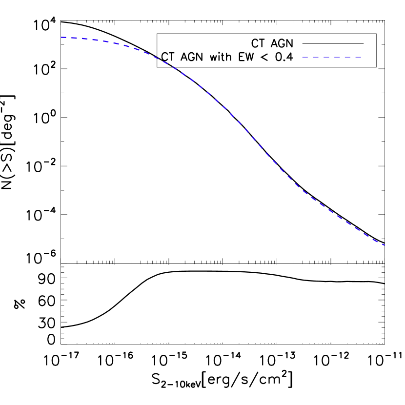
Figure 7.— Cumulative surface density of CT AGN (intrinsic rest-frame 2-10 keV luminosity above 10⁴² erg/s and HI column density above 10²⁴ cm^-2) and CT AGN with 6.2 $\mu$m aromatic feature EW lower than 0.4 (from which the AGN mid-IR featureless emission can be detected).

The featureless mid-IR emission from the dusty torus of AGN has been a powerful way to infer the intrinsic accretion luminosity. Especially when appearing along with weak or no X-ray emission, this continuum offers a strong indicator of CT HI columns (Lacy et al., 2004; Stern et al., 2005; Alonso-Herrero et al., 2006; Treister et al., 2009b; Alexander et al., 2008). Figure 5 gives the predicted median and 20-80% probability range of 6.2 $\mu$m aromatic feature EW of CT AGN in three intrinsic X-ray luminosity ranges, 10⁴²-10⁴³ erg/s, 10⁴³-10⁴⁴ erg/s and $>$ 10⁴⁴ erg/s. Note that the EW of star-forming templates in our model has a value of 0.6 $\mu$m, so smaller values indicate the presence of the contribution from the dusty torus. In Paper I, we compared our model’s predictions on the EW distributions to observations for two Spitzer legacy programs (GOALS & 5MUSES) and found a general consistency. Figure 5 also gives the observed EW of individual CT AGN drawn from the literature, where the local sample is from Risaliti et al. (1999), and high-z sample is from Alexander et al. (2008). Although a fair comparison between the model and observation is impossible for such a sample, the data are within the model predicted range. Figure 6 further shows the 6.2 $\mu$m feature EW distribution of AGN above different intrinsic X-ray luminosities. We define objects with EW_6.2μm $<$ 0.4 $\mu$m as those with detectable hot dust emission from AGN, because observations confirm a small scatter in the star-forming 6.2 $\mu$m EWs, with the median of 0.6 $\mu$m and 3-$\sigma$ dispersions about 0.2-0.25 $\mu$m (e.g. Wu et al., 2010; Stierwalt et al., 2013). The figure indicates that the fractions of CT AGN that have EW_6.2μm $<$ 0.4, i.e., detectable AGN mid-IR emission, are 27%, 55%, 98% and 100% for the limiting intrinsic rest-frame 2-10 keV luminosities of 10⁴², 10⁴³, 10⁴⁴ and 10⁴⁵ erg/s, respectively. Thus almost all intrinsically luminous CT AGN (unobscured $L_{\rm rest-2-10keV}$ $>$ 10⁴⁴ erg/s) have detectable AGN mid-IR emission, consistent with recent IR studies of high luminosity AGN (Mateos et al., 2013). Figure 7 shows the fraction of CT AGN with EW_6.2μm $<$ 0.4 $\mu$m as a function of the 2-10 keV flux. Above 10^-15 erg/s/cm² where intrinsic bright CT AGN dominate, 80-90% of CT AGN have EW_6.2μm $<$ 0.4 $\mu$m. Below 10^-15 erg/s/cm², the fraction drops with decreasing fluxes but still remains appreciable, around 60% and 30% at 2-10 keV flux of 10^-16 erg/s/cm² and 10^-17 erg/s/cm², respectively.

The reliable identification of CT AGN beyond the local universe is still a challenge, even though multi-wavelength tools that combine the X-ray data with optical/IR photometry have been developed to reveal many candidates. The upper panel of Figure 8 shows the distribution of AGN in the plane of log($f_{\rm 2-10keV}/f_{\rm 0.5-2keV}$) vs. log($f_{\rm IRAC8{\mu}m}/f_{\rm 0.5-2keV}$). The median positions of AGN with log($N_{\rm HI}$/cm^-2)=21.5, 22.5, 23.5, 24.5 and 25.5 are labelled. Heavily obscured AGN ($N_{\rm HI}$ $>$ 10²³ cm^-2) are predicted to be well separated from the unobscured and mildly obscured objects ($N_{\rm HI}$ $<$ 10²³ cm^-2). Note that in our model, the range in the distribution of a given $N_{\rm HI}$ is mainly caused by variation in the redshift-dependent K correction and contamination by star formation in the IRAC-8$\mu$m band. It does not incorporate the effect of variation in the AGN SED at X-ray and IR wavelengths. Also shown in Figure 8 are the locations of the CDFS sources from Xue et al. (2011), which spread over a large region in this plane. However, the distributions of observed CT AGN candidates as compiled from Alexander et al. (2008, 2011) roughly lie within our predicted range of heavily-obscured AGN, supporting the idea that heavily-obscured AGN can be identified through this simple diagnostic. The validity of a similar diagnostic plot has also been proposed by Severgnini et al. (2012) based on photometry of local confirmed Compton-thick AGN. In the lower panel of Figure 8, we also examine the validity of log($f_{\rm 20-40keV}/f_{\rm 0.5-2keV}$) vs. log($f_{\rm IRAC8{\mu}m}/f_{\rm 0.5-2keV}$) in separating AGN with different HI columns, which has a similar ability to the above diagnostic as shown in the upper panel.

Launched in June 2012, NuSTAR (Harrison et al., 2013) should quickly help constrain the distribution of CT AGN. Figure 9 shows the predicted redshift distribution of all AGN and CT AGN above three flux limits targeted in NuSTAR surveys, namely $f_{10-30keV}$ $>$ 2$\times$10^-14, 4$\times$10^-14 and 1.5$\times$10^-13 erg/s/cm². Given 0.3, 1-2 and 3 square degree for those three flux limits, respectively, our model predicts $\sim$100 AGN in total but only a few CT AGN that will be detected by NuSTAR at 10-30 keV. Our predicted total number of AGN is similar to to recent predictions by Ballantyne et al. (2011), but our predicted number of CT AGN is lower than theirs with the amount of the difference (a factor of 2-5) depending on the X-ray LFs they adopted.

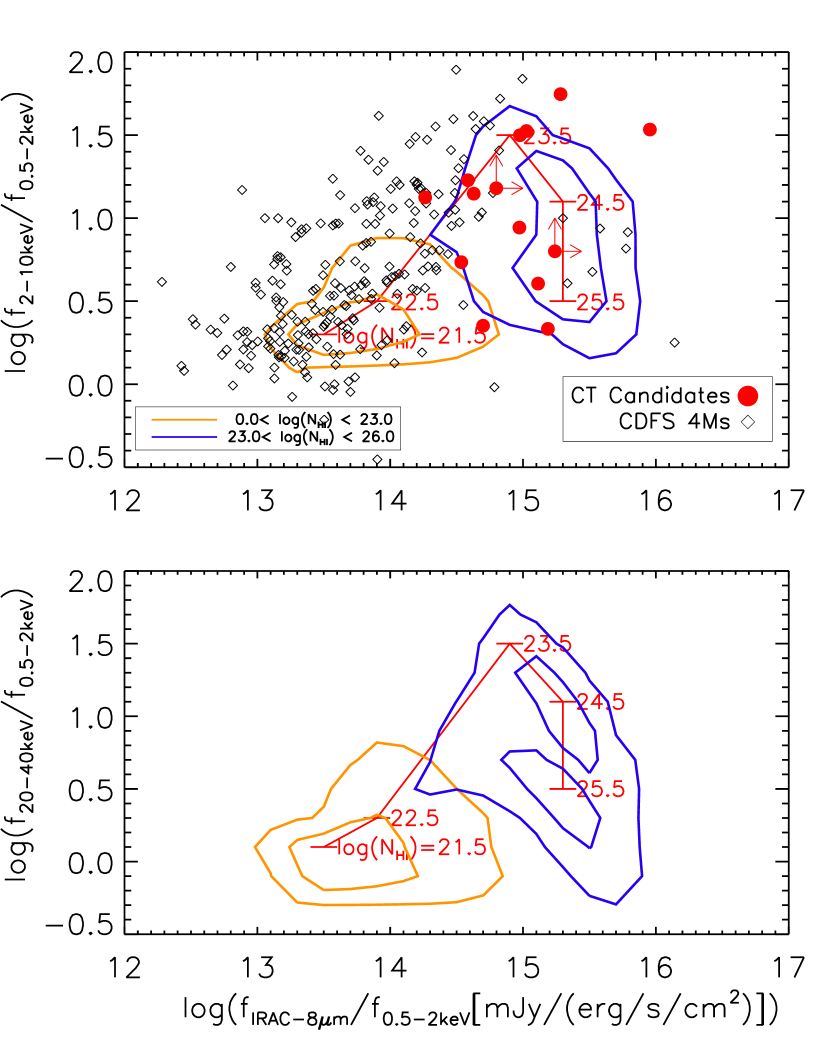
Figure 8.— Distribution of AGN with different HI columns in the X-ray hardness vs. IR/X-ray ratio plane: log$(f_{\rm 2-10keV}/f_{\rm 0.5-2keV})$ vs. log$(f_{\rm IRAC-8{\mu}m}/f_{\rm 0.5-2keV})$ for the upper panel and log$(f_{\rm 20-40keV}/f_{\rm 0.5-2keV})$ vs. log$(f_{\rm IRAC-8{\mu}m}/f_{\rm 0.5-2keV})$ for the lower panel. Orange and green contours are for unobscured and mildly-obscured AGN (log$N_{\rm HI}$ $<$ 23) and heavily-obscured AGN (log$N_{\rm HI}$ $>$ 23), respectively. For each contour, two levels enclose 60% and 90% of objects, respectively. The diamond symbols give distributions of all CDF-S sources (Xue et al., 2011) while filled circles are CT AGN candidates from Alexander et al. (2008, 2011).

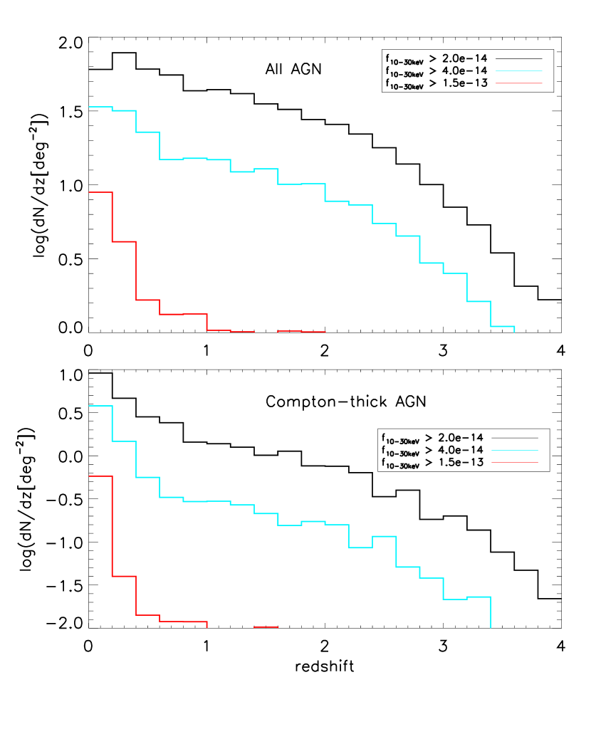
Figure 9.— Predicted redshift distribution of NuSTAR AGN (upper panel) and NuSTAR CT AGN (lower panel) for three survey depths as listed in Harrison et al. (2013).

6. Conclusions

We employ our joint population model of X-ray and IR backgrounds to predict the CT AGN abundance and compare it to a diverse set of empirical determinations. The main conclusions are:

(1) At intrinsic $L_{\rm rest2-10keV}$ $>$ 10⁴² erg/s, the CT AGN density is predicted to be around a few $\times$10^-4 Mpc^-3. The density of higher luminosity CT AGN increases rapidly from $z$=0 to $z$$\sim$2-3 and peaks at higher $z$.

(2) The CT AGN fraction appears to be low (2-5% ) at $f_{\rm 2-10keV}$ $>$ 10^-15 erg/s/cm² but increases rapidly at fainter flux levels.

(3) The SMBH accretion in CT AGN accounts for 38% of the total accreted SMBH mass and contributes to 25% of the CXB spectrum at its peak.

(4) We also investigate the mid-IR spectra of CT AGN based on techniques that have been developed to identify CT objects. The model predicts that the majority (90%) of bright CT AGN ($L_{\rm rest2-10keV}$ $>$ 10⁴⁴ erg/s or $f_{\rm 2-10keV}$ $>$ 10^-15 erg/s/cm²) have detectable hot dust emission from dusty tori; the fraction drops for faint objects, reaching 30% at $L_{\rm rest2-10keV}$ $>$ 10⁴² erg/s or $f_{\rm 2-10keV}$ $>$ 10^-17 erg/s/cm². Based on this, we confirm that heavily obscured AGN ($N_{\rm HI}$ $>$ 10²³ cm^-2) can be separated from lower HI column AGN through the plane of the observed-frame X-ray hardness vs. mid-IR/xray ratio.

7. Acknowledgment

We thank the anonymous referee for helpful comments that improve the paper significantly. The work is supported through the Spitzer 5MUSES Legacy Program 40539. The authors acknowledge support by NASA through awards issued by JPL/Caltech.

References

- Ajello et al. (2008) Ajello, M., et al. 2008, ApJ, 689, 666
- Ajello et al. (2012) Ajello, M., Alexander, D. M., Greiner, J., et al. 2012, ApJ, 749, 21
- Alexander et al. (2008) Alexander, D. M., et al. 2008, ApJ, 687, 835
- Alexander et al. (2011) Alexander, D. M., Bauer, F. E., Brandt, W. N., et al. 2011, ApJ, 738, 44
- Alonso-Herrero et al. (2006) Alonso-Herrero, A., Pérez-González, P. G., Alexander, D. M., et al. 2006, ApJ, 640, 167
- Ballantyne et al. (2011) Ballantyne, D. R., Draper, A. R., Madsen, K. K., Rigby, J. R., & Treister, E. 2011, ApJ, 736, 56
- Barger et al. (2005) Barger, A. J., Cowie, L. L., Mushotzky, R. F., Yang, Y., Wang, W.-H., Steffen, A. T., & Capak, P. 2005, AJ, 129, 578
- Brightman & Ueda (2012) Brightman, M., & Ueda, Y. 2012, MNRAS, 423, 702
- Comastri et al. (1995) Comastri, A., Setti, G., Zamorani, G., & Hasinger, G. 1995, A&A, 296, 1
- Churazov et al. (2007) Churazov, E., et al. 2007, A&A, 467, 529
- Daddi et al. (2007) Daddi, E., et al. 2007, ApJ, 670, 173
- Draper & Ballantyne (2009) Draper, A. R., & Ballantyne, D. R. 2009, ApJ, 707, 778
- Draper & Ballantyne (2010) Draper, A. R., & Ballantyne, D. R. 2010, ApJ, 715, L99
- Elmegreen & Burkert (2010) Elmegreen, B. G., & Burkert, A. 2010, ApJ, 712, 294
- Fabian (1999) Fabian, A. C. 1999, MNRAS, 308, L39
- Fiore et al. (2009) Fiore, F., et al. 2009, ApJ, 693, 447
- Förster Schreiber et al. (2006) Förster Schreiber, N. M., Genzel, R., Lehnert, M. D., et al. 2006, ApJ, 645, 1062
- Gendreau et al. (1995) Gendreau, K. C., et al. 1995, PASJ, 47, L5
- Genzel et al. (2008) Genzel, R., Burkert, A., Bouché, N., et al. 2008, ApJ, 687, 59
- Georgantopoulos et al. (2009) Georgantopoulos, I., Akylas, A., Georgakakis, A., & Rowan-Robinson, M. 2009, A&A, 507, 747
- Gruber et al. (1999) Gruber, D. E., Matteson, J. L., Peterson, L. E., & Jung, G. V. 1999, ApJ, 520, 124
- Gilli et al. (2007) Gilli, R., Comastri, A., & Hasinger, G. 2007, A&A, 463, 79
- Guainazzi et al. (2005) Guainazzi, M., Matt, G., & Perola, G. C. 2005, A&A, 444, 119
- Harrison et al. (2013) Harrison, F. A., Craig, W. W., Christensen, F. E., et al. 2013, ApJ, 770, 103
- Hasinger et al. (2005) Hasinger, G., Miyaji, T., & Schmidt, M. 2005, A&A, 441, 417
- Hopkins et al. (2007) Hopkins, P. F., Richards, G. T., & Hernquist, L. 2007, ApJ, 654, 731
- Hopkins et al. (2012) Hopkins, P. F., Hayward, C. C., Narayanan, D., & Hernquist, L. 2012, MNRAS, 420, 320
- Lacy et al. (2004) Lacy, M., Storrie-Lombardi, L. J., Sajina, A., et al. 2004, ApJS, 154, 166
- Law et al. (2007) Law, D. R., Steidel, C. C., Erb, D. K., et al. 2007, ApJ, 669, 929
- Luo et al. (2011) Luo, B., Brandt, W. N., Xue, Y. Q., et al. 2011, ApJ, 740, 37
- Mainieri et al. (2002) Mainieri, V., Bergeron, J., Hasinger, G., et al. 2002, A&A, 393, 425
- Marconi et al. (2004) Marconi, A., Risaliti, G., Gilli, R., Hunt, L. K., Maiolino, R., & Salvati, M. 2004, MNRAS, 351, 169
- Mateos et al. (2013) Mateos, S., Alonso-Herrero, A., Carrera, F. J., et al. 2013, MNRAS, 434, 941
- Moretti et al. (2009) Moretti, A., et al. 2009, A&A, 493, 501
- Perola et al. (2004) Perola, G. C., Puccetti, S., Fiore, F., et al. 2004, A&A, 421, 491
- Piccinotti et al. (1982) Piccinotti, G., Mushotzky, R. F., Boldt, E. A., et al. 1982, ApJ, 253, 485
- Piconcelli et al. (2003) Piconcelli, E., Cappi, M., Bassani, L., Di Cocco, G., & Dadina, M. 2003, A&A, 412, 689
- Polletta et al. (2006) Polletta, M. d. C., et al. 2006, ApJ, 642, 673
- Risaliti et al. (1999) Risaliti, G., Maiolino, R., & Salvati, M. 1999, ApJ, 522, 157
- Revnivtsev et al. (2003) Revnivtsev, M., Gilfanov, M., Sunyaev, R., Jahoda, K., & Markwardt, C. 2003, A&A, 411, 329
- Severgnini et al. (2012) Severgnini, P., Caccianiga, A., & Della Ceca, R. 2012, A&A, 542, A46
- Shankar et al. (2004) Shankar, F., Salucci, P., Granato, G. L., De Zotti, G., & Danese, L. 2004, MNRAS, 354, 1020
- Shi et al. (2013) Shi, Y., Helou, G., Armus, L., Stierwalt, S., & Dale, D. 2013, ApJ, 764, 28
- Stern et al. (2005) Stern, D., Eisenhardt, P., Gorjian, V., et al. 2005, ApJ, 631, 163
- Stierwalt et al. (2013) Stierwalt, S., Armus, L., Surace, J. A., et al. 2013, ApJS, 206, 1
- Tacconi et al. (2010) Tacconi, L. J., Genzel, R., Neri, R., et al. 2010, Nature, 463, 781
- Tozzi et al. (2006) Tozzi, P., et al. 2006, A&A, 451, 457
- Treister et al. (2009a) Treister, E., Urry, C. M., & Virani, S 2009, ApJ, 696, 110
- Treister et al. (2009b) Treister, E., Cardamone, C. N., Schawinski, K., et al. 2009, ApJ, 706, 535
- Treister et al. (2010) Treister, E., Natarajan, P., Sanders, D. B., et al. 2010, Science, 328, 600
- Türler et al. (2010) Türler, M., Chernyakova, M., Courvoisier, T. J.-L., Lubiński, P., Neronov, A., Produit, N., & Walter, R. 2010, A&A, 512, A49
- Wada & Norman (2002) Wada, K., & Norman, C. A. 2002, ApJ, 566, L21
- Wu et al. (2010) Wu, Y., et al. 2010, ApJ, 723, 895
- Xue et al. (2011) Xue, Y. Q., Luo, B., Brandt, W. N., et al. 2011, ApJS, 195, 10
- Yu & Tremaine (2002) Yu, Q., & Tremaine, S. 2002, MNRAS, 335, 965