Statistics of weighted Poisson events and its applications

Abstract

The statistics of the sum of random weights where the number of weights is Poisson distributed has important applications in nuclear physics, particle physics and astrophysics. Events are frequently weighted according to their acceptance or relevance to a certain type of reaction. The sum is described by the compound Poisson distribution (CPD) which is shortly reviewed. It is shown that the CPD can be approximated by a scaled Poisson distribution (SPD). The SPD is applied to parameter estimation in situations where the data are distorted by resolution effects. It performs considerably better than the normal approximation that is usually used. A special Poisson bootstrap technique is presented which permits to derive confidence limits for observations following the CPD.

and

1 Introduction

In the analysis of the data collected in particle experiments, frequently weighted events have to be dealt with. For instance, losses due to a limited acceptance of the detector are  corrected by weighting each events by the inverse of its detection probability. The sum of the weights is used to estimate the number of incident particles. Frequently an event cannot be uniquely assigned to a signal or to a background and is attributed a weight. It is necessary to associate confidence limits, upper or lower limits to the sum of these weights and we want to apply goodness-of-fit tests to histograms of weighted events. When data are compared  to different theoretical predictions, weighting simplifies the computation and sometimes it is unavoidable. Of special importance is parameter estimation from histograms where the measured variable is distorted by the limited resolution and acceptance of the detector. To evaluate these effects, Monte Carlo simulations have to be performed. In the simulation a p.d.f. $f_{0}(x)$ is assumed to describe the data where $x$ represents the set of event variables that are measured. The simulation often requires considerable computer power. To change the p.d.f. of the simulation to $f(x)$, the simulated events are weighted by  $f(x)/f_{0}(x)$. This is unavoidable if $f(x|\theta)$ depends on one or several parameters $\theta$ that have to be estimated. During the fitting procedure where the experimental distributions are compared to the simulated ones, the parameters and correspondingly the weights $f(x|\theta)/f(x|\theta_{0})$ are varied.

The distribution of the sum $x$ of a Poisson distributed number of weights is described by a compound Poisson distribution (CPD), provided the weights can be considered as independent and identical distributed random variables. This condition is realized in the majority of experimental situations. The CPD applies to a large number of problems. In astrophysics, for instance, the total energy of random airshowers follows a CPD. Also outside physics the CPD is widely used to model processes like the sum of claims in car accidents and other insurance cases which are assumed to occur randomly with different severity.

Usually we do not dispose of the distribution of the weights but have to base the analysis on the observed weights of a sample of events. The mean value and the variance of the weighted sum can be inferred directly from the corresponding empirical values, but in many cases a more detailed knowledge of the distribution is necessary. To deal with these situations, the approximation of the CPD by a scaled Poisson distribution and a special bootstrap technique are proposed.

In the first part of this article some properties of the CPD and an approximation of it that is useful in the analysis of experimental data are discussed. The second part contains applications where observed samples of weights have to be analyzed and where the underlying distribution of the weights is unknown. Parameter estimation with weighted Monte Carlo events using a scaled Poisson distribution and the estimation of confidence limits with Poisson bootstrap are studied.

2 The compound Poisson distribution

2.1 Distribution of a sum of weighted Poisson numbers

The distribution of a weighted Poisson number $x=wm$ with $m\sim\mathcal{P}_{\lambda}(m)=e^{-\lambda}\lambda^{m}/m!$, $m=0,1,2,\ldots$ and the weight $w$, a real valued positive parameter, $w>0$ is

$$W(x)=\frac{e^{-\lambda}\lambda^{x/w}}{(x/w)!}\;.$$

To evaluate the moments of the Poisson distribution, it is convenient to use the cumulants. The moments $\mu_{k}$ of a distribution are polynomials of the cumulants $\kappa_{1,}...,\kappa_{k}$ of the distribution. For the first two moments $\mu,\sigma^{2}$, the skewness $\gamma_{1}$ and the excess $\gamma_{2}$ the relations are $\mu=\kappa_{1}$, $\sigma^{2}=\kappa_{2}$, $\gamma_{1}=\kappa_{3}/\kappa_{2}^{3/2}$, $\gamma_{2}=\kappa_{4}/\kappa_{2}^{2}$. The cumulants $\kappa_{k}$ of the Poisson distribution $\mathcal{P}_{\lambda}$ are especially simple, they are all identical and equal to the mean value $\lambda$ and thus $\gamma_{1}=1/\lambda^{1/2}$ and $\gamma_{2}=1/\lambda$. From the homogeneity of the cumulants follows for the cumulant $\kappa_{k}(x)$ of order $k$ of the distribution of $x$ the relation $\kappa_{k}(x)=\kappa_{k}(wm)=w^{k}\lambda$.

We consider now two Poisson processes with random variables $n_{1}$ and $n_{2}$ and mean values $\lambda_{1}$ and $\lambda_{2}$. We are interested in the distribution of the weighted sum $x=x_{1}+x_{2}=w_{1}n_{1}+w_{2}n_{2}$ with positive weights $w_{1}$, $w_{2}$.

The mean value and the variance of $x$ are

$$\mathrm{E}(x) =w_{1}\lambda_{1}+w_{2}\lambda_{2}\;,$$ (1)

$$\mathrm{Var}(x) =w_{1}^{2}\lambda_{1}+w_{2}^{2}\lambda_{2}\;.$$ (2)

These results follow from the properties of expected values and are intuitively clear. The cumulant of the distribution of the sum of two independent random variables $x_{1}$ and $x_{2}$ is the sum of the two cumulants:

$$\kappa_{k}=w_{1}^{k}\lambda_{1}+w_{2}^{k}\lambda_{2}\;.$$ (3)

Relation (3) can be generalized to $N$ Poisson processes with mean values $\lambda_{i}$:

$$\kappa_{k}={\displaystyle\sum\limits_{i=1}^{N}}w_{i}^{k}\lambda_{i}\;.$$ (4)

We will see below that the case is of special interest where all mean values $\lambda_{i}$ are equal. With $\lambda_{i}=\lambda/N$, and $x=\Sigma w_{i}$ the modified relation for the cumulants is

$$\kappa_{k}=\lambda\Sigma w_{i}^{k}/N=\lambda\left\langle w^{k}\right\rangle\;,$$ (5)

and $\mu$, $\sigma$, $\gamma_{1}$,$\gamma_{2}$ are:

$$\mu =\lambda\Sigma_{i}w_{i}/N=\lambda\left\langle w\right\rangle\;,$$ (6)

$$\sigma^{2} =\lambda\Sigma_{i}w_{i}^{2}/N=\lambda\left\langle w^{2}\right\rangle\;,$$ (7)

$$\gamma_{1} =\frac{\lambda\Sigma_{i}w_{i}^{3}/N}{\sigma^{3}}=\frac{\left\langle w^{3}\right\rangle}{\lambda^{1/2}\left\langle w^{2}\right\rangle^{3/2}}\;,$$ (8)

$$\gamma_{2} =\frac{\lambda\Sigma_{i}w_{i}^{4}/N}{\sigma^{4}}=\frac{\left\langle w^{4}\right\rangle}{\lambda\left\langle w^{2}\right\rangle^{2}}\;.$$ (9)

Here $\left\langle v\right\rangle$ denotes the mean value $\Sigma_{i=1}^{N}v_{i}/N$.

So far we have treated the weights as parameters, while according to the definition of a compound Poisson process, the weights are random variables.

2.2 Distribution of the sum of random weights

In most applications of particle physics the distribution of the sum of individually weighted events is of interest. The number $n$ of events is described by a Poisson distribution and to each event a random weight is associated. Instead of the $N$ independent Poisson processes with mean values $\lambda_{i}$ and random variables $n_{i}$ we can consider the random variable $n=\Sigma n_{i}$ as the result of a single Poisson process with $\lambda=\Sigma\lambda_{i}$. The numbers $n_{i}$ are then chosen from a multinomial distribution where $n$ is distributed to the $N$ different weight classes with probabilities $\varepsilon_{i}=\lambda_{i}/\lambda$, i.e. a weight $w_{i}$ is chosen with probability $\varepsilon_{i}$:

$$W(n_{1},...,n_{N}) ={\displaystyle\prod_{i=1}^{N}}\mathcal{P}(n_{i}|\lambda_{i})=\mathcal{P}_{\lambda}(n)\mathcal{M}_{\varepsilon_{1},...,\varepsilon_{N}}^{n}(n_{1},...,n_{N})\;,$$ (10)

$$\mathcal{M}_{\varepsilon_{1},...,\varepsilon_{N}}^{n}(n_{1},...,n_{N}) =n!{\displaystyle\prod\limits_{i=1}^{N}}\varepsilon_{i}^{n_{i}}\left/{\displaystyle\prod\limits_{i=1}^{N}}n_{i}!\right.\;.$$ (11)

The validity of (10) is seen from the following identity for the binomial case,

$$\mathcal{P}_{\lambda}\mathcal{M}_{\lambda_{1}/\lambda,\lambda_{2}/\lambda}^{n}=\frac{e^{-\lambda}\lambda^{n}}{n!}\frac{n!}{n_{1}!n_{2}!}\frac{\lambda_{1}^{n_{1}}\lambda_{2}^{n_{2}}}{\lambda^{n_{1}}\lambda^{n_{2}}}=\frac{e^{-(\lambda_{1}+\lambda_{2})}\lambda_{1}^{n_{1}}\lambda_{2}^{n_{2}}}{n_{1}!n_{2}!}=\mathcal{P}_{\lambda_{1}}\mathcal{P}_{\lambda_{2}}\;$$

which is easily generalized to the multinomial case.

It does not matter whether we describe the distribution of $x$ by independent Poisson distributions or by the product of a single Poisson distribution with a multinomial distribution. If all probabilities are equal, $\varepsilon_{i}=1/N$, the multinomial distribution describes a random selection of the weights $w_{i}$ out of the $N$ weights with equal probabilities $1/N$. The formulas (6) to (9) remain valid.

To describe a continuous weight distribution $f(w)$ with finite variance, the limit $N\rightarrow\infty$ has to be considered. Again our formulas remain valid with $\varepsilon N=1$. We get $x=\Sigma_{i=1}^{n}w_{i}$. The mean values $\left\langle w^{k}\right\rangle$ in (5), (6), (7), (8), (9) are to be replaced by the corresponding expected values $\mathrm{E}(w^{k})$, e.g. the moments of the weight distribution.

3 Approximation by a scaled Poisson distribution

To analyze the sum of weights of observed samples where the underlying weight distribution is not known, it is necessary to approximate the CPD. According to the central limit theorem, the sum of weighted Poisson random numbers with mean number $\lambda$ and expected weight $\mathrm{E}(w)$ can asymptotically, for $\lambda\rightarrow\infty$, be described by a normal distribution with mean $\mu=$ $\lambda\mathrm{E}(w)$ and variance $\sigma^{2}=\lambda\mathrm{E}(w^{2})$, provided the expected values exist. The speed of convergence with $\lambda$ depends on the distribution of the weights.

As is demonstrated below, the moments of the CPD are closer to those of a scaled Poisson distribution (SPD) than to the moments of the normal distribution. Especially, if the weight distribution is narrow, the SPD is a very good approximation of the CPD and in the limit where all weights are identical, it coincides with the CPD.

The SPD is fixed by the requirement that the first two moments of the CPD have to be reproduced. We define an equivalent mean value $\tilde{\lambda}$,

$$\tilde{\lambda} =\lambda\frac{\mathrm{E}(w)^{2}}{\mathrm{E}(w^{2})}$$ (12)

$$=\mu\frac{\mathrm{E}(w)}{\mathrm{E}(w^{2})}=\frac{\mu}{s}\;,$$ (13)

an equivalent random variable $\tilde{n}\sim\mathcal{P}_{\tilde{\lambda}}$, a scale factor $s$,

$$s=\frac{\mathrm{E}(w^{2})}{\mathrm{E}(w)}\;,$$ (14)

and a scaled random variable $\tilde{x}=s\tilde{n}$ such that the expected value $\mathrm{E}(\tilde{x})=\mathrm{E}(x)=\mu$ and the variance $\mathrm{Var}(\tilde{x})=\mathrm{Var}(x)=\sigma^{2}$. The cumulants of the scaled distribution are $\tilde{\kappa}_{k}=s^{k}\tilde{\lambda}$.

To evaluate the quality of the approximation of the CPD by the SPD, we compare the cumulants of the two distributions and form the ratios $\kappa_{k}/\tilde{\kappa}_{k}$. Per definition the ratios for $k=1,2$ agree because the two lowest moments agree.

The skewness and excess for the two distributions in terms of the expected values of powers $k$ of $w$, $\mathrm{E}(w^{k})$ are according to (8), (9) and (12):

$$\gamma_{1} =\frac{\mathrm{E}(w^{3})}{\lambda^{1/2}\mathrm{E}(w^{2})^{3/2}}\;,$$ (15)

$$\gamma_{2} =\frac{\mathrm{E}(w^{4})}{\lambda\mathrm{E}(w^{2})^{2}}\;,$$ (16)

$$\tilde{\gamma}_{1} =\frac{1}{\tilde{\lambda}^{1/2}}=\left[\frac{\mathrm{E}(w^{2})}{\lambda\mathrm{E}(w)^{2}}\right]^{1/2}\;,$$ (17)

$$\tilde{\gamma}_{2} =\frac{1}{\tilde{\lambda}}=\frac{\mathrm{E}(w^{2})}{\lambda\mathrm{E}(w)^{2}}\;.$$ (18)

For the ratios we obtain

$$\frac{\gamma_{1}}{\tilde{\gamma}_{1}} =\frac{\mathrm{E}(w^{3})\mathrm{E}(w)}{\mathrm{E}(w^{2})^{2}}\geq 1\;,$$ (19)

$$\frac{\gamma_{2}}{\tilde{\gamma}_{2}} =\frac{\mathrm{E}(w^{4})\mathrm{E}(w)^{2}}{\mathrm{E}(w^{2})^{3}}\geq 1\;.$$ (20)

The proof of these inequalities is given in the Appendix. As $\gamma_{1}$ and $\gamma_{2}$ of the normal distribution are zero, the values $\gamma_{1}$ and $\gamma_{2}$ of the CPD are closer to those of the SPD than to those of the normal distribution. This property suggests that the SPD is a better approximation to the CPD than the normal distribution. According to the central limit theorem, CPD and SPD approach the normal distribution with increasing $\tilde{\lambda}$. The equalities in (19) and (20) hold if all weights are equal. Remark that the ratios do not depend on the expected number $\lambda$ of weights, only the moments of the weight distribution enter. The ratios are close to unity in most practical cases. They can become large if the weight distribution comprises weights that differ considerably and especially if many small weights are combined with few large weights. This is the case, for instance, for an exponential weight distribution.

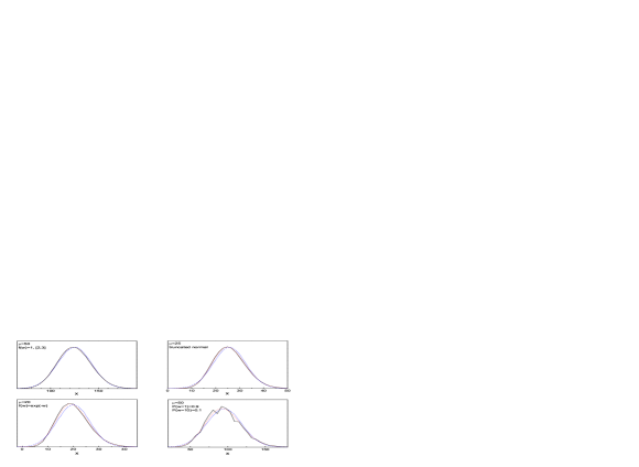
Figure 1: Comparison of a CPD (solid) with a SPD (dotted) and a normal distribution (dashed)

In Figure 1 the results of a simulation of CPDs with different weight distributions is presented. The simulated events are collected into histogram bins but the histograms are displayed as line graphs which are easier to read than column graphs. Corresponding SPD distributions are generated with the parameters chosen according to the relations (12) and (14). They are indicated by dotted lines. The approximations by normal distributions are shown as dashed lines. Due to the discrete Poisson distribution the histograms for the composite Poisson distribution and the SPD have pronounced structures that makes it difficult to compare the results. To avoid at least partially this disturbing effect, the binning was adapted to the steps of the SPD. The weight distribution of the top left graph is uniform in the interval $[2,3]$ and the weight distribution of the top right graph is a truncated, renormalized normal distribution $\mathcal{N}_{t}(x|1,1)=c\mathcal{N}(x|1,1)$, $x>0$ with mean and variance equal to $1$ where negative values are cut. In both cases the approximation by the SPD is hardly distinguishable from the CPD. In the bottom left graph the weights are exponentially distributed. This case inhibits large weights with low frequency where the approximation by the SPD is less good. Still it models the CPD reasonably well. In the bottom right  graph the weight distribution is discrete with the weight $w_{1}=1$ chosen with probability $0.9$ and the weight $w_{2}=10$ chosen with probability $0.1$. This is again an extreme situation. The SPD and the CPD agree reasonably well globally, but have different discrete structures which result in jumps caused by the binning. The examples show, that the approximation by the SPD is mostly close to the CPD and that it is always superior to the approximation by the normal distribution.

In Table 1 we compare skewness $\gamma_{1}$ and excess $\gamma_{2}$ of the SPD to the values of the CPD. The mean values from $1000000$ simulated experiments are taken. The mean number of weights is always $50$, e.g. $n\sim\mathcal{P}_{50}(n)$. The weights used to obtain the first $3$ rows are uniformly distributed in the indicated interval. The weights of the following row are distributed according to $\exp(-w)$, the weights of the next row follow the truncated normal distribution. The last two rows correspond to two discrete weights, $w_{1}=$ $1$ and $w_{2}=10$ chosen with equal probabilities and with $w_{1}=0.8$ and $w_{2}=0.2$, respectively. The second column indicates the number of equivalent events $\tilde{\lambda}$ defined in (12), e.g. the number of unweighted events with the same relative uncertainty as the weighted sum $x$. For example, the relative fluctuation $\delta x/x$ of the sum $x$ of $n\sim\mathcal{P}_{50}(n)$ random weights with $w\sim\exp(-w)$ is $1/\sqrt{25}=0.2$. The following columns contain the values of $\gamma_{1}$ and $\gamma_{2}$ of the CPD and those from the scaled Poisson distribution. The values of the normal approximation are $\gamma_{1}=\gamma_{2}=0$. The first two moments are per definition equal for the CPD and the SPD.

Table 1: Skewness and excess of the SPD approximation

type of weight	$\tilde{\lambda}$	$\gamma_{1}$	$\gamma_{2}$	$\tilde{\gamma}_{1}$	$\tilde{\gamma}_{2}$
$u[0,1]$	$37.50$	$0.184$	$0.036$	$0.163$	$0.027$
$u[1,2]$	$48.21$	$0.149$	$0.023$	$0.144$	$0.021$
$u[2,3]$	$49.34$	$0.144$	$0.021$	$0.142$	$0.020$
$exp(-w)$	$25.00$	$0.300$	$0.120$	$0.200$	$0.040$
$\mathcal{N}_{t}(1,1)$	$36.48$	$0.199$	$0.045$	$0.166$	$0.027$
$1$ $(p=0.5)$, $10$	$29.94$	$0.197$	$0.039$	$0.182$	$0.033$
$1$ $(p=0.8)$, $10$	$19.01$	$0.299$	$0.092$	$0.229$	$0.052$

The SPD values are close to the nominal values if the weight distribution is rather narrow corresponding to $\tilde{\lambda}/\lambda$ close to one. Remark that in the cases where the ratio $\tilde{\lambda}/\lambda$ is small, skewness and excess are relatively large and correspondingly, the normal approximation with $\gamma_{1}=\gamma_{2}=0$ is not very good. As in the limit $n\rightarrow\infty$ both, the CPD and the SPD, approach the normal distribution, small event numbers, or, more precisely, small values of $\tilde{\lambda}$ are especially critical.

4 The Poisson bootstrap

In standard bootstrap ([3]) samples are drawn from the observed observations $x_{i}$, $i=1,2,...,n$, with replacement. Poisson bootstrap is a special re-sampling technique where to all $n$ observation $x_{i}$ Poisson distributed numbers $n_{i}\sim\mathcal{P}_{1}(n_{i})=1/(en_{i}!)$ are associated. More precisely, for a bootstrap sample the value $x_{i}$ is taken $n_{i}$ times where $n_{i}$ is randomly chosen from the Poisson distribution with mean equal to one. Samples where the sum of outcomes is different from the observed sample size $n$, e.g. $\Sigma_{i=1}^{n}n_{i}\neq n$ are rejected. Poisson bootstrap is completely equivalent to the standard bootstrap. It has attractive theoretical properties [4].

In our case the situation is different. We do not dispose of a sample of CPD outcomes but only of a single observed value of $x$ which is accompanied by a sample of weights. As the distribution of the number of weights is known up to the Poisson mean, the bootstrap technique is used to infer parameters depending on the weight distribution, To generate observations $x_{k}$, we have to generate the numbers $n_{i}\sim$ $\mathcal{P}_{1}(n_{i})$ and form the sum $x=\Sigma n_{i}w_{i}$. All results are kept. The resulting Poisson bootstrap distribution (PBD) permits to estimate uncertainties of parameters and quantiles of the CPD. Mean values derived from an infinite number of simulated experiments and the moments extracted from the corresponding PBDs would reproduce exactly the moments of the CPD.

5 Applications

In most applications we do not know the weight distribution and have to infer it approximately from a sample of weights, $w_{i},i=1,...,n$. To this end we replace the moments of the weight distribution by the empirical values. A general approach to approximate the distribution of a sample starting from the cumulants is to apply the Edgeworths [1, 2] series. Since this method is involved and not directly related to the Poisson distribution, it has not been investigated. The Gram-Charlier series B [1] contains explicitly a Poisson term, but it is not clear how well the truncated series approximates the CPD. Furthermore the higher empirical cumulants $\kappa_{3},\kappa_{4},...$ in most applications suffer from rather large statistical fluctuations. Therefore it is often more precise to use the values tied to the mean and the variance in the approximation by the SPD. In addition to the SPD, we consider the simple normal approximation and Poisson bootstrap.

5.1 Parameter estimation from distorted measurements

An important application of the statistics of weighted events is parameter estimation in experiments where the data are distorted by resolution effects [5]. Typically, an experimental histogram with $m_{j}$ entries in bin $j$ has to be compared to a theoretical prediction $x_{j}(\theta)$ depending on one or several parameters $\theta$. The prediction is obtained from a Monte Carlo simulation which reproduces the experimental conditions and especially the smearing by resolution effects. The variation of the prediction with the parameter cannot be implemented by repeating the complete simulation for each selected parameter. Therefore the simulated data which are generated with the parameter $\theta_{0}$ according to the p.d.f. $f(\theta_{0})$ are re-weighted by the ratio $w=$ $f(\theta)/f(\theta_{0})$. The prediction for a histogram bin $j$ is then $x_{j}=\Sigma_{i=1}^{n_{j}}w_{ji}$ for $n_{j}$ generated events in bin $j$. To perform a least square fit of $\theta$ to a histogram with $B$ bins, we form a $\chi^{2}$ expression where we compare Poisson numbers $m_{j}$ times a known normalization constant $c$ to compound Poisson numbers $x_{j}$.

$$\chi^{2} ={\displaystyle\sum\limits_{j=1}^{B}}\frac{(cm_{j}-x_{j}(\theta))^{2}}{\delta_{j}^{2}}\;,$$

$$={\displaystyle\sum\limits_{j=1}^{B}}\frac{\left(cm_{j}-{\displaystyle\sum\limits_{i=1}^{n_{j}}}w_{ji}\right)^{2}}{\delta_{j}^{2}}\;.$$

Here $\delta_{j}^{2}$ is the expected value of the numerator under the hypothesis that the two summands in the bracket have the same expected value $\mu$. To estimate $\delta_{j}^{2}$ first $\mu$ has to be estimated.

In the normal approximation, we compute the weighted mean of the two summands (We suppress the index $j$.):

$$\hat{\mu}_{N}=\left(\frac{cm}{c^{2}m}+\frac{\Sigma w_{i}}{\Sigma w_{i}^{2}}\right)/\left(\frac{1}{c^{2}m}+\frac{1}{\Sigma w_{i}^{2}}\right)\;.$$ (21)

In the approximation based on the SPD, the value of $\mu$ can be estimated from an approximated likelihood expression. The log likelihood is [5]

$$\ln L(\mu)=m\ln\frac{\mu}{c}-\frac{\mu}{c}+\tilde{n}\ln\tilde{\lambda}-\tilde{\lambda}+const.$$ (22)

where it is assumed that $m$ follows a Poisson distribution with mean $\mu/c$ and $\tilde{n}=x/s$ a Poisson distribution with mean $\tilde{\lambda}=\mu/s$, see (12), (14). The maximum likelihood estimate is [5]

$$\hat{\mu}_{SPD}=cs\frac{\tilde{n}+m}{c+s}$$ (23)

and the corresponding estimate of $\delta^{2}$ is

$$\hat{\delta}_{SPD}^{2}=cs(\tilde{n}+m)\;.$$

To evaluate the quality of the two approximations, $1000000$ experiments have been simulated for different combinations of event numbers and weight distributions. The results are summarized in Table 2. Here $\lambda_{n}$ and $\lambda_{m}$ are the expected numbers of data and Monte Carlo events, $\mu$ is the mean value of $x$ that has been used in the simulation and that should be reproduced by the estimates, $\hat{\mu}_{SPD}$ is the mean value of the SPD estimates for $\mu$, $\sigma_{SPD}$ is the standard deviation of the estimates and $\hat{\mu}_{N},\sigma_{N}$ are the corresponding values for the normal approximation. The notation of the weight distributions is the same as above. All estimates of $\mu$ are negatively biased but as expected the SPD values are considerably closer to the nominal values than those of the normal approximation. The bias for  the SPD is in all cases below $3\%$ which is certainly adequate for the estimation of the uncertainty $\delta$. The fluctuations are anyway much larger than the biases both for the SPD and the normal distribution. Both approximations are adequate, the approximation with the SPD is slightly superior to that with the normal approximation and leads to a simple result of the estimate of the variance $\hat{\delta}^{2}$. Independent of the weight distribution the biases decrease with increasing number of events. In most cases it will be possible to generate a sufficient number of events such that $\tilde{\lambda}$ is of the order of $50$ or larger.

Table 2: Comparison of the SPD and the normal approximations

$\lambda_{n}$	$\lambda_{m}$	weight	$\mu$	$\hat{\mu}_{SPD}$	$\sigma_{SPD}$	$\hat{\mu}_{N}$	$\sigma_{N}$	$\frac{\hat{\mu}_{SPD}-\mu}{\mu}$	$\frac{\hat{\mu}_{N}-\mu}{\mu}$
$20$	$20$	$exp(-x)$	$20$	$19.98$	$3.68$	$19.10$	$3.84$	$0.001$	$0.045$
$10$	$10$	$exp(-x)$	$10$	$9.73$	$2.64$	$9.11$	$2.81$	$0.027$	$0.089$
$10$	$50$	$exp(-x)$	$10$	$9.88$	$1.38$	$9.58$	$1.59$	$0.012$	$0.042$
$20$	$50$	$exp(-x)$	$20$	$19.84$	$2.61$	$19.46$	$2.74$	$0.008$	$0.027$
$50$	$50$	$exp(-x)$	$50$	$49.78$	$5.79$	$49.12$	$5.91$	$0.004$	$0.013$
$10$	$10$	$\mathcal{N}_{t}(1,1)$	$12.88$	$12.78$	$3.13$	$12.05$	$3.30$	$0.008$	$0.068$
$20$	$20$	$\mathcal{N}_{t}\mathcal{(}1,1)$	$25.75$	$25.67$	$4.40$	$24.93$	$4.53$	$0.003$	$0.032$
$20$	$50$	$\mathcal{N}_{t}(1,1)$	$25.75$	$25.69$	$3.22$	$25.27$	$3.31$	$0.002$	$0.019$
$10$	$10$	$u[2,3]$	$25.00$	$25.00$	$5.61$	$23.74$	$5.87$	$0.000$	$0.050$
$20$	$20$	$u[2,3]$	$50.00$	$50.00$	$7.94$	$48.74$	$8.13$	$0.000$	$0.025$
$50$	$50$	$u[2,3]$	$125.00$	$125.01$	$12.54$	$123.75$	$12.67$	$0.000$	$0.010$

5.2 Approximate confidence limits

In searches for rare events frequently the identification is not unique and to each event is attributed a weight which corresponds to the probability to be correctly assigned. The underlying weight distribution is not known. Of interest is the number of produced events $x=\Sigma w_{i}$ and confidence limits for this number. The limits can be computed from the Poisson bootstrap distribution.

As an example, a sample of $n$ weights, with $n\sim\mathcal{P}_{50}(n)$ has been generated with a uniform weight distribution in the interval $[0,1]$. The value $x_{obs}=\Sigma_{i=1}^{n}w_{i}=22.01$ was obtained. The frequency plot of the corresponding bootstrap distribution $f(x)$ is displayed in Fig. 2 left hand side. This distribution was used to derive the error and confidence limits presented in Table 3. The limits corresponding to the $\alpha$ quantiles $x$, defined by $\alpha=F(x)=\int_{0}^{x}f(x^{\prime})dx^{\prime}$, indicated in the top line of the table, are quoted in the second line. The usual standard error interval is $18.2<x<25.8$.

Classical confidence intervals with exact coverage cannot be computed as the full CPD is known only approximately. But as we know the type of the distribution for the number of events, we can improve the coverage in the following way: We change the Poisson distribution used to generate the bootstrap samples from $\mathcal{P}_{1}$ to $\mathcal{P}_{\mu}$ such that the fraction of  outcomes $x$ below $x_{obs}\mathcal{\ }$is equal to $\alpha$. The upper limit is then $x_{up}=$ $x_{obs}\times\mu$. In a similar way the lower limit $x_{low}$ is obtained. The central interval $x_{low}<x<x_{up}$ should then contain the unknown true value with confidence $1-2\alpha$. In the limit where all weights are equal and the number of bootstrap samples tends to infinity the interval would cover exactly. The obtained limits are contained in the third line of the table. The two procedures lead to very similar values. The modified error inteval is now $18.5<x<26.2$. As expected from the properties of the Poisson distribution, the intervals with improved coverage are shifted to higher values.

Table 3: Confidence limits

$\alpha$	0.01	0.05	0.10	0.1585	0.8415	0.90	0.95	0.99
PBD	13.8	16.0	17.2	18.2	25.8	26.9	28.5	31.4
PBD*	14.4	16.5	17.6	18.5	26.2	27.3	28.9	32.1

The Poisson bootstrap can be used to estimate distributions of all kinds of parameters of the distribution. As an example the distribution of the skewness derived from the observed weight sample is presented in the right hand plot of Fig. 2.

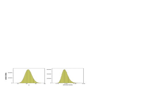
Figure 2: Bootstrap distribution of the random variable $x$(left hand)and of $\gamma_{1}$(right hand).

6 Summary

The sum of random weights where the number of weights is Poisson distributed is described by a compound Poisson distribution. Properties of the CPD are reviewed. The CPD is relevant for the analysis of weighted events that has to be performed in various physics applications.

It is shown that with increasing number of events the distribution of the sum can be approximated by a scaled Poisson distribution which coincides with the CPD in the limit where all weights are equal. Contrary to the normal distribution it approximately reproduces also the higher the moments of the CPD. The SPD can be applied to the parameter estimation in situations where the data are distorted by resolution effects. The formalism with the SPD is simpler than that with the normal approximation and the results are more precise. This has been demonstrated for examples with various weight distributions.

A special bootstrap method is presented which can be used to estimate from experimental samples parameters of the underlying CPD. An example shows how it can be applied to the estimation of confidence limits.

7 Appendix: Proof of the Inequalities (19) and (20)

We apply Hölders inequality,

$$\sum_{i}a_{i}b_{i}\leq\left(\sum_{i}a_{i}^{p}\right)^{1/p}\left(\sum_{i}b_{i}^{p/(p-1)}\right)^{(p-1)/p}\;,$$

where $a_{i},b_{i}$ are non-negative and $p>1$. For $p=2$ we obtain the Cauchy–Schwartz inequality. Setting $a_{i}=w_{i}^{3/2}$, respectively $b_{i}=w_{i}^{1/2}$, we get immediately the relation (19) for the skewness:

$$\left(\sum_{i}w_{i}^{2}\right)^{2}\leq\sum_{i}w_{i}^{3}\sum_{i}w_{i}\;.$$

More generally, with $p=n-1$ and $a_{i}=w_{i}^{n/(n-1)}$, $b_{i}=w_{i}^{(n-2)/(n-1)}$, the inequality becomes

$$\left(\sum_{i}w_{i}^{2}\right)^{n-1}\leq\sum_{i}w_{i}^{n}\left(\sum_{i}w_{i}\right)^{n-2}\;.$$

This formula includes also the relation (20) for $n=4$.

References

- [1] M.G. Kendall and A. Stuart, The Advanced Theory of Statistics, Charles Griffin & Co., London, Ed. 4 (1948).
- [2] E.W. Weisstein, Edgeworth Series, http://mathworld.wolfram.com; en.wikipedia.org/wiki/Edgeworth_series.
- [3] B. Efron and R.T. Tibshirani, An Introduction to the Bootstrap, Chapman& Hall, London (1993).
- [4] G.J. Babu et al., Second-order correctness of the Poisson bootstrap, The Annals of Statistics Vol 27, No. 5 (1999) 1666.
- [5] G. Bohm and G. Zech, Comparing statististical data to Monte Carlo simulation with weighted events, Nucl. Instr. and Meth A691 (2012) 171.