The SUMER Data in the SOHO Archive

Abstract

We have released an archive of all observational data of the VUV spectrometer Solar Ultraviolet Measurements of Emitted Radiation (SUMER) on SOHO that has been acquired until now. The operational phase started with ‘first light’ observations on 27 January 1996 and will end in 2014. Future data will be added to the archive when they become available. The archive consists of a set of raw data (Level 0) and a set of data that are processed and calibrated to the best knowledge we have today (Level 1). This communication describes step by step the data acquisition and processing that has been applied in an automated manner to build the archive. It summarizes the expertise and insights into the scientific use of SUMER spectra that has accumulated over the years. It also indicates possibilities for further enhancement of the data quality. With this article we intend to convey our own understanding of the instrument performance to the scientific community and to introduce the new, standard-FITS-format database.

1 Introduction

sec: Intro

The Solar Ultraviolet Measurements of Emitted Radiation (SUMER; Wilhelm et al., 1995) telescope and spectrometer has been taking ultraviolet spectra (50 nm to 161 nm) from the Solar and Heliospheric Observatory (SOHO) since its launch in December 1995. The complete dataset up to January 2013 has been reprocessed and is now available in FITS format from the SOHO archive. The motivation and basic idea behind this communication is to describe aspects of the data acquisition that are relevant to the data quality and details of the various steps and procedures needed to arrive at Level 1 (L1) data. The data reduction steps used in the archive correspond to the best knowledge of today. Even after so many years, the processing is still not perfect and at several stages compromises had to be taken, which may explain why this task was not completed earlier.

SUMER data has so far been accessible from archives that contain reformatted telemetry, i.e. raw, Level 0 (LZ) data that is provided either in FITS, FTS, or IDL restore format. Various correction and calibration procedures have to be applied in order to minimize the known instrumental effects in LZ data and to convert the incoming signal to physical quantities of the radiation. The basic knowledge acquired during ground testing and commissioning was continuously extended, confirmed, or improved over the years. This knowledge is documented in almost 1000 articles in refereed journals as indicated in Figure fig:publ. There are clear indications from the publication rate that also future work with SUMER data can be expected. It is our motivation to make sure that the accumulated knowledge will not be forgotten, and at the same time provide ready-to-use spectra to the community for future work.

Figure 1.: Record of refereed publications. Entries listed by ESA under SUMER/SOHO are given as solid line, whereas those in ADS are denoted as diamonds. The year 2013 is shown with special symbols, because the figures are not final. The graph stands for the experience accumulated over the years, which is the base of the archive.fig:publ

Details of the reduction procedures were made publicly available on the instrument web sites. The latest update was in 2008. The procedures used to produce L1 data described here represent the present view of our instrument. A fair amount of this information is presented as a complete, overworked and self-standing document. We cannot exclude deviations from the results of data processing that was completed in earlier times. The differences are to our knowledge small and will in all likelihood not affect the validity of previous analyses. Therefore, this improved view of our instrument in no way compromises reduction work with previous versions, but does also not claim to be final. For this reason we have tried to make the description of each individual step as transparent as possible. This may help the user not to use the reduction as a black box, but to improve the results if future insights allow him to do so.

The application of the various correction and calibration procedures has to reverse the order applied to the incoming signal by the various instrument subsystems. This applies in particular to stages of the signal processing in the detectors with specific shortcomings (procedures 2 to 6). Therefore the sequence must be executed in the described order:
1. Decompression
2. Deadtime correction
3. Odd-even pattern
4. Local-gain correction
5. Flatfield correction
6. Geometric distortion correction
7. Radiometric calibration

If at a later time, an improvement in any one of these procedures is possible, then either the raw data can be reprocessed with the improved algorithm or the existing correction must be re-tracked to the problematic procedure that has to be replaced and re-run together with those following in the sequence. All information needed for the re-tracking is documented in the FITS header of L1 data.

In addition to these procedures that affect the pixel values themselves, we also mention procedures that are to be used for special analyses, but have not been applied to the archive data. These are procedures to compensate for the instrumental effect on the width of spectral lines, to compute the movement of the slit image as parasitic effect of the grating focus mechanism, to estimate the stray-light level in off-limb spectra, and give information on the wavelength calibration including thermo-elastic deformation effects along the spectral dimension.

2 Instrument Description

sec: Instrument

The instrument is described in Wilhelm et al. (1995). Performance details are given in Wilhelm et al. (1997a) and Lemaire et al. (1997). The concept of the instrument is also discussed and reviewed in the general context of VUV space instrumentation in Wilhelm et al. (2004). A survey of the most significant results is found in Wilhelm et al. (2007). Here we emphasize those details that are relevant to the archive. The particular spectral range that is covered by SUMER comprises emission lines and continua of many elements. It includes the entire Lyman series of hydrogen and chromospheric emission from other atomic constituents, as well as emission lines useful for observations of transition-region or coronal phenomena. It turned out that forbidden transitions between high-lying levels of highly ionized iron and other heavy species can be used as proxies for X-ray radiation and tracers of processes during flare events (Feldman et al., 2000), thus supporting X-ray spectroscopy.

2.1 Optical Design

sec: Optics

The optical design of the instrument is shown in Figure fig:opt and discussed in Wilhelm et al. (1995). Many features hereof are relevant for instrumental effects and are important for the data reduction. The optical system is based on a normal-incidence off-axis telescope and a slit spectrometer in Wadsworth mount. Pointing is accomplished by two nested mechanisms that allow, for optical performance reasons, a spherical motion of the parabolic mirror around the changeable slit in the focal plane. The beam issued from the slit – entrance of the spectrometer – is collimated by an off-axis parabolic mirror. The collimated beam is seen by a spherical concave grating producing a stigmatic image of the slit that is dispersed in wavelength. A plane mirror in front of the grating allows us to change the angle of incidence and thus, to modify the setting of the instantaneous wavelength portion seen by the detectors in the focal plane of the grating. The effective focal length of the grating depends on the angle of incidence and thus on the wavelength setting. A grating focus mechanism is, therefore, needed to keep the spectral image on the detector always in focus. For this reason, important optical parameters are wavelength dependent, notably the magnification, the angular pixel size along the slit, and the dispersion defining the spectral pixel size. All these parameters are provided in the FITS header of the data files.

The reduction of scattered light has been a strong requirement for the optical system and the surface quality of the optical components with chemical-vapor-deposited (CVD) silicon carbide (SiC) coated surfaces. Measurements of the surface roughness performed at GSFC (Saha and Leviton, 1993) have shown that the rms micro-roughness at 10 $\mu$m scaling length was 0.6 nm, which is well within the specification. Such measurements have been used to predict the scatter performance at FUV wavelengths.

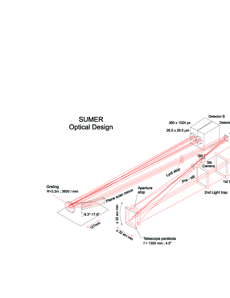
Figure 2.: Layout of the optical system. The diagram shows the extreme rays of the folded beam and indicates the position and movement of the mechanisms serving the system.fig:opt

2.2 Mechanisms

sec: Mechanisms

SUMER is equipped with seven mechanisms, the door mechanism, two mechanisms for pointing in azimuth and elevation, the slit changer, the telescope focus mechanism, the wavelength scan, and the grating focus. All mechanisms are actuated by stepper motors and have position encoders for monitoring purposes. The encoders are operated in open-loop modes, i.e., the positions that are read out are telemetered as housekeeping values, but not used to control the stepper motors.

2.2.1 Pointing in Azimuth and Elevation

pointing

With incremental single steps of 0.38^′′ both in azimuth and elevation, the telescope could be pointed anywhere in the field of view of 64^′ $\times$ 64^′ centred on the Sun. The azimuth drive was also used to scan regions of interest on the Sun and to compensate for the solar rotation in sit-and-stare applications. The nominal elevation pointing position is always related to the central pixel of the slit, irrespective of the location of the slit image on the detector.

The absolute pointing uncertainty of typically 10^′′ is the combined result of thermoelastic effects on SOHO as well as in the instrument, of step losses in the mechanism, and of the parasitic shift of the slit image on the detector resulting from a misalignment of the grating focus mechanism (as described below). From time to time and for special cases the solar limb was used to ‘re-calibrate’ the reference position of the SUMER pointing mechanism (the zero position of the SUMER coordinate system).

When step losses of the azimuth drive occurred in October 1996, it was decided to operate the driving motor with retaining power and in high-current mode. Only sporadic step losses occurred over the succeeding years in this mode. However, in April 2008, the problem re-appeared ex nihilo and became worse since then. Raster scans could not reliably be completed anymore. With the help of the azimuth position encoder, pointing was still possible. The value of the azimuth and elevation encoders are given in the L1 image header in order to improve the knowledge of the pointing. We note, however, that the encoder reading for the housekeeping process is completed at a cadence of 15 s and not synchronized with the science operation. With short exposure times it may happen that the encoder values in the first image header are not yet updated.

2.2.2 Slit Focus and Slit Select

slit

During the commissioning phase in early 1996, the slit focus mechanism was used to optimize the focus position of the telescope (cf., Lemaire et al., 1997). The setting has not been changed since then. The slit changer can choose between the four slits of size 4^′′ $\times$ 300^′′, 1^′′ $\times$ 300^′′, 1^′′ $\times$ 120^′′, and 0.3^′′ $\times$ 120^′′. Images of the short slits can be positioned in such a way that the top, the central, or the bottom section of the detector active area are illuminated, ‘top’ or ‘bottom’ settings are called ‘asymmetric’ slit positions. In bottom position, a baffle obscures the extreme pixels of the short slits (#5 and #8). The slit selection constrains the image format that is appropriate for the detector readout. Possible image formats including their telemetry load are listed in Table tab:formats. The low telemetry rate of $10.5\times 10^{3}$ bits per second turned out to be a major limitation for fast data acquisition. Faster raster scans could, however, be completed by buffering spectra into the on-board memory up to a data volume of $\approx 5\times 10^{6}$ bytes.

Table 1.: Standard image formats. Other formats that are only used for special applications are not listed here. The telemetry-load column applies for the nominal TM rate of $10.5\times 10^{3}$ bits per second.tab:formats

ID	Spectral pixels	Spatial pixels	Format	TM load
				s
2	1024	360	1 byte	280.9
3	1024	360	2 bytes	561.8
4	1024	120	1 byte	93.7
5	1024	120	2 bytes	187.3
8	50	360	1 byte	13.8
9	50	360	2 bytes	27.5
10	50	120	1 byte	4.6
11	50	120	2 bytes	9.2
12	25	120	1 byte	6.9
13	25	120	2 bytes	13.8
14	25	120	1 byte	2.3
15	25	120	2 bytes	4.6
37	256	360	2 bytes	140.5
38	512	360	1 byte	140.5
39	512	360	2 bytes	280.9

2.2.3 Wavelength and Grating Focus

grating

The optical system requires that the wavelength and grating focus mechanisms are always operated simultaneously. Because of a misalignment of the grating focus drive – a combination of the misalignment of the guiding rails of the grating focus mechanism, the rotational axis of the wavelength mechanism, and the grating optical axis – the position of the slit image on the detector is slightly offset, whenever a new wavelength setting is commanded. The combined effect of this parasitic movement and the change of the angular pixel size is up to 25 pixels as shown in Figure fig:shift (see also Section 5.4). Since the readout window is fixed and does not follow the shift, often dark pixels appear in short-slit image formats.

Figure 3.: Parasitic pixel displacement of the slit image over the spectral range.fig:shift

When only partial spectral windows are transmitted, the line of interest should in an ideal case be centred in the telemetered window. This is normally not the case and one should keep in mind that the repeatability of this mechanism is limited (see Section 5.4.1). At short wavelengths, one actuator step corresponds to seven spectral pixels, while several steps are needed for a shift of one pixel at the other extreme. Therefore, problems with the wavelength setting occur more often in the short wavelength range.

2.3 Detectors

sec: XDL

SUMER is equipped with two photon-counting detector systems. Details of the detectors and their performance are given in Siegmund et al. (1994). A triple stack of multichannel plates (MCP) carries the photocathode deposited on the front face of the first MCP and a cross delay-line anode converts photons to an electronic pulse. The travel time of the pulse through the crossed delay-lines determines the location of the photon event and the image is constructed by a time-to-digital converter (TDC) that creates a 1024 $\times$ 360 array of photon events, which we for simplification, but inaccurately call pixels. It is this analog-to-digital conversion and, in particular, the linearity of this ADC which, in part, is responsible for some of the artifacts in the digital image, most notably the odd-even pattern, as described below.

High overall count rates result in deadtime effects, since every individual event has to be processed by the post-anode digital electronic and bright lines will lead to local gain depression of the MCPs. The adverse effects of these shortcomings are balanced or even overcompensated by a unique feature of photon counting systems: their dark signal is almost negligible so that deep exposures can be made with very low signal. In other words, the dynamic range can be extended over many orders of magnitude.

A sample spectrum around 118 nm is shown in Figure fig:xdl to illustrate the layout of the detector array. Only the most prominent lines are indicated (cf., Curdt et al., 2001, for a comprehensive line identification). The slit image covers only $\approx$300 out of the 360 spatial pixels. The central spectral pixels ($\approx$280 to $\approx$770) represent those sections, where the KBr photocathode is deposited on the bare MCP. These pixels have a much higher sensitivity, in particular in the spectral range from 90 nm to 130 nm (see Section 6 for details). Some pixels at the bare-to-KBr transition are difficult to interpret, since this is not a sharp boundary. The extreme 50 pixels on both sides are covered by a grid that serves as an 1:10 attenuator. However, as a side effect the attenuation exerts a modulation on the line profile, which makes it difficult to interpret these data.

Figure 4.: Sample data of a full frame image showing the detector layout. The image has been reversed in wavelength and detector effects have been corrected. The spectral range from 116.0 nm to 120.4 nm comprises the He i line at 58.4 nm, observed in second order of diffraction. In this spectral range, the efficiency of the central, KBr-coated section is significantly enhanced. The 1:10 attenuation affects 50 pixels on both extremes (cf., Section 5.4.1 for wavelength calibration). The image is part of a QS dataset obtained on 20 April 1997 (cf., Curdt et al., 2001, for details).fig:xdl

SUMER is also equipped with a rear slit camera (RSC). Despite misalignment problems, which reduced the scientific value of this device, the RSC could be used to verify the pointing mechanism by locating sunspots and by observing the solar limb. In the archive, RSC images are only included as raw data.

2.4 Instrument Operation

sec: Operation

The principal data acquisition features of SUMER are described in detail in Wilhelm et al. (1995). The instrument operation applied during the many years of observation is summarized hereafter. During several years (1996 to 2003), the 24 h of SOHO throughput operation was divided in a long pass with continuous real-time access during at least 8 h and two or three small 1 h real-time passes. Later, the real-time coverage was reduced and became more irregular. The round-trip time for real-time commands is about 10 s with an uplink rate of three bytes per second. The on-board SUMER memory capability was 64 elementary or macro commands (formatted as User Defined Programme, see the following UDP section). So, at any time during a real-time pass we have been able to load instantaneous or time-tagged activities. The primary ground station to operate the instrument is located at the GSFC/EOF (Experiment Operation Facility at the Goddard Space Flight Center). During few campaigns remote terminals at the IAS/MEDOC (Multi-Experiment Data and Operation Centre at the Institut d’Astrophysique Spatiale) could be connected to this station. Since 2011 we can also operate our instrument remotely from MPS. The operations were completed following a timeline comprising a time span of $\approx$24 h. The definition of the timeline was accomplished in several steps.

2.4.1 Target Selection and Definition of the Type of Observation

Target selection was done by looking at the status of the Sun with the image-tool routine. Image-tool is the user interface of a pointing tool that is based on a database of solar images obtained from ground-based and space observatories, e.g. SOHO/Extreme ultraviolet Imafing Telescope (EIT; Delaboudinière et al., 1995) and allows fine targeting for an observation to come hours or days in advance. The choice of the feature (coordinates and times) to be observed was done by the SUMER observer or in coordination with other SOHO (or other ground-based or space observatory) instruments.

2.4.2 SUMER Command Language, Predefined and User-Defined Programmes

A dedicated command language has been used to define the structure and contents of observing sequences. A library of high-level functions specific to SUMER and elements to build loops, branching points, etc. are the basic features of the SUMER command language (SCL). Various mapping modes and other elements of the SCL library are described in Wilhelm et al. (1995). The SCL source code to define an observing sequences is written in plain English. It sets the telescope pointing coordinates, the selected entrance slit of the spectrometer, the reference pixel on the detector associated with a wavelength, the wavelength and the associated windows on the detector, the exposure times, the number of spectra to be collected, and the detector voltage handling. A set of 30 differently structured, hard-wired observing sequences, so-called Predefined Observational Programmes (POPs) was already included in the SUMER flight software. Some had a simple linear structure, but more complex ones with loops and branching points were also available. In addition, new User-Defined Programmes (UDPs), also written in SCL code, could be added to the available POPs after passing different stages of a validation process. First, the syntax was checked, then the code was compiled and converted to a token code as input to the TKI (Token Code Interpreter) programme, a tool that is also part of the on-board software. Finally, the token code of each new UDP had to pass an instrument simulator before the sequence was added to the pool of more than 1000 validated UDPs. In addition to the POPs, the token code of 16 different UDPs could be held on board at the same time.

Unfortunately, a flaw in the detector communication occasionally terminated the full execution of a POP. Mitigation of this problem required to modify the hard-wired structure of the code and this could only be completed by rewriting the sequence as UDP. The availability of such user-defined sequences demonstrated the enormous flexibility of the software design and turned out to be highly appropriate for the operation of SUMER. Most of the time, SUMER was operated in this mode. Any spectrum in the archive is linked to its ‘mother’ UDP, which is kept in the UDP database (cf., Section 2.6).

2.4.3 Generation and Uploading of Commands

The prepared observation programmes are inserted into the SUMER Planning Tool, which can generate a file of time-tagged execution commands to be sent to the SUMER on-board computer through a SOHO channel opened by the SOHO/EOF ground system. At the same time, an activity plan can be produced to be loaded into the SOHO activity data base, documenting the plan to be executed.

2.4.4 Monitoring and Preprocessing of Real-Time Data

A few seconds after the observation the real-time data are collected and displayed on ground computers (EOF, MEDOC, MPS). Few minutes after the data are taken, they are pre-processed using a quick-look facility to follow the progress of the observations. That has been very useful in order to react in near real-time to the selection of sunspot coordinates, the solar limb position (using the rear slit camera) or the selection of any solar feature within a raster scan image. In parallel house keeping data are received in real-time and are used to follow the instrument parameter and to detect any anomaly that requires an operator reaction, either to check the accomplishment of the programme and re-iterate the observation as needed or to optimize parameters for a secondary run of that programme.

2.5 Ground Support Facilities

sec: EGSE

The ground support facilities were built as a dual Electrical Ground Support Equipment (EGSE): a scientific EGSE based on a VMS operating system (here referenced as operation station) and a PC-based maintenance EGSE. The maintenance EGSE is used for real-time commanding and real-time visualization of scientific and housekeeping data necessary to check the health of the instrument and the running of the observational programme. The operation station was used to complete scientific observations: target selection, creation of UDP, insertion of individual commands and programmes in the time line through the Planning Tool, sending the commands, reception of the telemetry, pre-processing the raw scientific data in the Quick-Look and formatting the zero level FITS (FTS) data to feed the preliminary SOHO archive. The dual EGSE was duplicated at the IAS/MEDOC centre.

2.6 UDP Database

sec: UDP

The source code of all used UDPs is accessible on the MPS SUMER archive web page. These files are not needed directly for the FITS formatting process. Information about, which programme is used to acquire the dataset is included in the FITS image header (see Section sec: Aux).

2.7 The Archive

sec: Archive intro

The SUMER archive is part of the total SOHO archive which is built around the archive created by all SOHO instruments. The main SOHO archive is based at NASA/GSFC, while a copy is maintained at ESA and at IAS/MEDOC. The access to the SUMER LZ archive can be accomplished through various web pages.

3 Data Resources

sec: Data

In this chapter it is described which data sources are included in the processing from TM raw data to the ready FITS product. Further on it describes the various additional data sources which are processed and how this information is added to the FITS image header. A flow diagram showing the data sources and processing steps is depicted in Figure fig:dataflow.

3.1 TM Processing

sec: TM processing The SOHO telemetry data is distributed in files which contain the data of one day (see SOHO Interface Control Document). For SUMER there are three different kinds of file, standard housekeeping data called HK0 and science low and high rate files. The HK0 data are extracted out of the TM files and written, also on a daily base, into binary files. This is more or less a copy process. Processing the science data needs considerably more effort, since the SUMER image data packets are interlaced with science housekeeping packets (e.g. HK255, see SUMER Operations Guide, Chapter 5 for more detailed information). During processing the various packets are extracted and, depending on the type, are sorted into binary files for HK and images. The produced binary HK0, science HK, and image files build the base for all further processing and SUMER data products.

3.2 Science Data

sec: Science data

The main sources of SUMER data are the SOHO/SUMER telemetry (TM) files. These files consist of a header, the TM packets, information about telemetry gaps and information about the transmission quality of the packet as listed below. The gap and quality information are added to the SUMER image header in the flags QAC and MDU. If the QAC flag is set it means that during transmission an error occurred. When the MDU flag is set it means, there are TM packets missing and the image contains fill data at these positions. The fill data is chosen as the max value in the image. For traceability of the data processing, the name of the TM source file is added to the FITS header.
The reflecting FITS keywords are:

Keyword	Description
XSSMDU	Missing data in image 0=no,1=yes
XSSQAC	Quality of image data 0=OK,1=NOTOK
XSSFID	File ID from TM file catalog
XSSFPTR	Pointer to image position in bin file
XSCDID	CD ID of TM file
XSSEQID	CD sequence ID of TM file
XSTMFILE	TM filename without ext

3.3 Housekeeping Data

sec: HK The SUMER image header already contains a snapshot of most housekeeping values of the moment the image is taken. But there are still significant values missing, like temperatures of the instrument and the encoder positions of the mechanisms. These values are sampled every 15 s to 45 s and are sent asynchronously via the housekeeping channel HK0. The HK0 data are read and correlated to the start time of an exposure plus half of the exposure time so that they are accurate mid-way through the exposure. This approach is more accurate for exposure times longer than 1 min because of the sample rate of HK0 data. The maximum delay for the HK0 values is 300 s. This information is added to the FITS Header.

Keyword	Description
T3TELE	Telescope (MC2) temperature in degree Celsius
T3REAR	SUMER rear (MC3) temperature in degree Celsius
T3FRONT	SUMER front (MC4) temperature in degree Celsius
T3SPACER	SUMER spacer (MC6) temperature in degree Celsius
MC2ENC	SUMER MC2 (azimuth) encoder position
MC3ENC	SUMER MC3 (elevation) position
MC4ENC	SUMER MC4 (slit select) position
MC6ENC	SUMER MC6 (scan) encoder position
MC8ENC	SUMER MC8 (grating) encoder position
HK0TIME	Time stamp of HK0 record

3.4 Auxiliary Data

sec: Aux

The information about UDP name, campaign, etc. are extracted from the Oracle planning database and commanding log files. This data is formatted into FITS files (tables). This intermediate extraction step is done due to the fact that the SUMER planning database is not globally accessible, and the produced FITS files can be more easily distributed. These files will be put into the SSWDB area so the the information can be accessed with simple FITS read programmes (e.g. fits_read). The task of correlating the information by time, is done during processing (LZ preparation).

The routine update_fits completes the time correlation and adds the information to the FITS header. This routine calls the routines get_fitsudpinfo and get_fitscmpinfo, which read the information from the auxiliary FITS tables.

The information/keywords added to the header by update_fits are:

Keyword	Description
CMP_NAME	Name of campaign observation
CMP_ID	Campaign number
STUDY_ID	Study number (database ID)
STUDY_NM	Study name
OBJECT	Target
SCIENTIST	Scientist responsible of POP/UDP
OBS_PROG	Name of scientist programme
PROG_NM	Name of observing programme

The spacecraft attitude information are distributed as FITS files. Using the IDL routines get_sc_att and get_sc_point from Solar Software tree (SSW) the attitude information can be read and then added into the FITS header. The solar angles P0 and B0 are read with the routine pb0r and also added to the header.

Keyword	Description
SOLAR_P0	Solar angle P0 / deg
SOLAR_B0	Solar angle B0 / deg

Geocentric and heliocentric information is added from information read in with the function get_orbit.

4 Data Reduction Steps

sec: Reduction

Details of the data reduction steps that were used to prepare L1 data are described here. The order of the various data reduction steps follows the rational as explained before.

4.1 Decompression

sec: decompression

In most cases, the accumulated counts of the 16-bit data array have been compressed on board to 1-byte integers. The by far most often applied ‘Method 5’ (quasi-logarithmic byte scale) used an algorithm that mapped the dynamic range found in the image to a logarithmic lookup table. For numbers from 0 to 107 the result of the lookup table is a one-to-one copy of the input value. Thus all values with low count rates are preserved losslessly, and can be reversed by a decompression that uses information contained in the raw image header. Data in LZ format as well as in FITS and FTS format of existing archives are already decompressed during creation, if methods between 5 and 10 were employed. Data that was compressed by application of more complex compression methods (e.g. ‘moment calculation’) is only available in LZ format, since decompression is not possible.

4.2 Reversion

sec: Reversion

The pixel addresses of the SUMER detectors are such that the highest wavelength is on pixel 0, the lowest on pixel 1023; the wavelength stated in the raw header refers to the reference pixel. Therefore, wavelengths are descending from left to right in reformatted raw data. For compatibility with the SOHO conventions and the following image correction routines, the spectral direction of the images in LZ format of this archive and in FITS or FTS format has already been reversed (such that wavelength increases to the right).

4.3 Flatfield Correction and Removal of Digitization Nonlinearity

sec: FF

4.3.1 Image Features that Need a Correction by a Flatfield Routine

Detector anode and photocathode both show effects that are specific for each detector and are relevant for the data reduction. The flatfield correction of SUMER images generally corrects small-scale structures introduced by the detectors. Larger structures, like the overall response of the different photocathode areas, are treated by the radiometric calibration routine. The small-scale structures are introduced by the spatial inhomogeneity of the channel plate response and the non-linearity of the analog-to-digital converters of the detector electronics. Another small-scale structure that may be present in SUMER images, is local gain depression which, however, must be treated by another routine.

Inhomogeneity of the micro-channel plate response is mainly due to the hexagonal pattern of the microfiber bundles and the relative orientation of these bundles in a stack of three microchannel plates. Depending on this relative orientation, a complex moiré pattern of the response is produced, which is very distinct in the detector A and much less pronounced in the detector-B. If a clear hexagonal (‘chicken wire’) pattern is visible in the image it is produced by the lowest channel plate (the one which is closest to the anode). The smaller structures are produced by the superposition of the fiber bundles of the three plates.

In addition to the moiré pattern there may be dead pores in one of the channel plates, which lead to dark spots in the image. Depending on which of the plates has the dead pore determines the size of the dark spot. Because of the spreading of the charge, when transferred from one plate to the next, more pores are blacked-out in the succeeding plate and, thus the dark spot is larger when it is in the first plate (the one farthest from the anode).

The further processing of the signal to create a digital image out of the analog signal by the time-to-digital converter (TDC) leads to additional small-scale artifacts in the image data. A non-linearity of the analog-to-digital-converter (ADC) introduces a difference in the response between two succeeding rows of the image. This can be seen in the very distinctive alternating response of the odd and even rows of the image. The ADC non-linearity causes that the signal in one row is about 9.5 % higher than average, while in the adjacent row it is 9.5 % lower than average, thus making on average a 19 % difference between the rows. In the following, we will call this the ‘odd-even pattern’. Note that this pattern only exists in the rows of the image, not in the columns where it has been avoided internally by the detector electronics using an unsharpening technique (‘dithering’). This effect, which is present in both detectors, is also effectively averaged out if an even number of binning is applied along the slit direction. The non-linearity of the time-to-digital converter of the post-anode digital electronics is found to be constant in time and well characterized for both detectors. It can rather easily be removed. However, during the period from June 2005 to November 2006, when a flaw in the address decoder of detector A developed that rapidly progressed and finally led to the destruction of the TDC unit, the fixed pattern of this chain increased significantly. During this time period, the characteristic of the TDC was regularly monitored, so that these data are still scientifically sound. The best results were found by separation of both effects, when in a first step the pattern is compensated and in a second step the residual non-uniformities of the pixel array were removed.

4.3.2 Producing Flatfield Correction Data

There is no flatfield illumination of SUMER detectors on board. There are however alternative ways in producing quasi-flat illuminations of the SUMER detectors that can be used to extract the small-scale features and produce a data array that can be used to compensate these artifacts.

In order to produce a quasi-flat illumination of the detectors on board, an observing sequence has been written that puts the SUMER spectrograph in a state of maximal defocusing at the wavelength of 88 nm for a several-hour long observation of a preselected quiet-Sun (QS) area at the wavelength of the Lyman continuum. At this wavelength the solar spectrum is devoid of strong lines, and a quiet solar region avoids bright features with strong variability in the field of view. The defocusing provides a smearing of any small features to a size of at least 16 pixels. Thus, the resulting image of this deep exposure – an example is shown in Figure fig:ff – can be used to extract small-scale features of the detectors. An on-board routine extracts from this exposure the small-scale ‘fixed pattern’ by applying a median filter (of size 16 pixels) to the data and division by the filtered image. The resulting image (the flatfield array) is a matrix with values between 0.5 and 1.5, the average value being 1.0. It is stored on board for processing of images and sent to ground by telemetry for further application to any data on the ground. The flatfield correction array is applied in a simple multiplicative way. The procedure of flatfield correction can be made on ground (or, reversely, the on-board flatfield corrections can be undone) by using the function sum_flatfield.pro available in the Solar Software Tree.

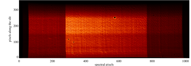
Figure 5.: Flatfield exposure of the detector A showing the moiré pattern of the MCPs and some smaller dark features. The dark spot is a cluster of low-gain pores. Note, extreme pixel addresses around the edges and the areas of the attenuators are not useable.fig:ff

Flatfield arrays have been produced frequently until 1998, but later the occasions of making flatfield exposures have been greatly reduced in an effort to reduce the total exposure of the detectors to high count rates that would lead to ever increasing high voltage needed to compensate for the resulting gain loss. As the high voltage power supply units were reaching their upper limits, at some occasions only short flatfield exposures have been taken, which could be used to find any changes in the flatfield structures with respect to the latest deep exposures.

Another method to determine the ‘fixed pattern’ of the detectors can be employed when a large enough data set can be used to extract from the average of all images, in a similar way as above, the small-scale features introduced by the detector. In general, this average of the images is not as deep an exposure as the ‘normal’ flatfield exposure of three hours in the Lyman continuum, but its one certain advantage is that it is as close in time as possible to the actual observations to which it will be applied. This is useful in particular cases, because not all of the ‘fixed patterns’ are really fixed in time.

4.3.3 Changes of the Fixed Pattern with Time

It had been found very early in 1996, by comparing several flatfield correction arrays of detector A, that the flatfield pattern of the detectors were changing slightly with the time of usage of the detector. This can be found by correlating with each other different flatfield array data. The correlation can be maximized by a shift of the flatfield pattern, which is mostly less than one pixel (in $X$- and $Y$-directions), but can amount to several pixels between different flatfields. There may be several reasons for this shift of the small-scale pattern: One reason lies in the ‘scrubbing’ of channel plates, i. e., extracting charge from the MCPs by heavy usage, and the resulting gain loss of the lowest of the three channel plates. Since the channels are inclined with respect to the anode, the gain loss may cause a shift of the charge cloud centroid that should be located on the anode by the position encoding. Such an effect was clearly detected when a strong spectral line was observed for long time at the same location on the detector. Then, the persisting gain loss at this location resulted in a shift of the charge cloud centroid towards the area with higher gain. Fortunately, the SUMER wavelength scan mechanism allows the position of spectral lines to be place anywhere on the detector and this resulted on the average to a more or less uniform gain loss across the active area. When such a uniform gain loss was reached, increasing the high voltage of the MCPs could compensate it. This gain calibration has been done frequently. But the change of high voltage may have an effect on the electrical field between the channel plate and the anode. It may also have an effect on the position encoding if it affects the travel time of pulses in the cross-delay lines of the position encoding system. Both may lead to a shift of the image pattern. Therefore, new flatfield images have been acquired regularly - roughly every month - after the high-voltage setting had been newly adjusted during a gain calibration. Later, when the observations of the solar disk have been reduced to save lifetime of the detectors, the period between flatfield acquisitions has been increased.

Since the gain loss occurs more or less constantly during usage of the detector and the compensation can only be done stepwise, there is, in principle, a possible small shift between the data and the flatfield pattern. But in general the shift of the flatfield pattern is not uniform. A uniform scrubbing of the detector cannot be achieved, and therefore a differential (or local) scrubbing, which is due to the non-uniform illumination of the detector during its use, results in a shift pattern that is not uniform: depending on which part of the detector area has been used more, the shift is higher in these areas. In addition, as mentioned above, the ‘fixed pattern’ results from a superposition of the pattern of each channel plate. The scrubbing, however, takes place mostly in the lowest channel plate (the one closest to the anode), from which the largest amount of charge has been drawn. Thus it may be possible that features arising from different channel plates may suffer a different displacement in the image. However, this intricacy may be difficult to detect, since the differences are probably much smaller than one pixel.

There is, however, a very strong fixed pattern in the flatfield data that never changes. It is the nonlinearity of the detector ADC in the position encoding electronics, which causes the difference of responsivity of odd and even rows. This odd-even pattern is always present along the slit direction, and it has been found to be very stable throughout the time of all flatfield images we have.

4.3.4 Application of the Flatfield Correction

The general flatfield routine sum_flatfield.pro applies to the image data the flatfield correction array in the same way as the on-board flatfield routine. It corrects all fixed pattern by multiplication of the flatfield correction array. It does not take into account any changes of the fixed pattern with time. Thus, it corrects perfectly the odd-even pattern and much of the other channel plate non-uniformities. By selecting the flatfield array dated closest to the date of observation, the shift between the flatfield data and the corrected data can be minimized. This is the simplest approach, and for most purposes the results are satisfactory.

To improve the flatfield correction, we can take the shift of the fixed pattern into account. In this case, the odd-even pattern must be corrected first. For this purpose we have extracted the odd-even pattern from the flatfield raw data and produced new flatfield arrays that have the odd-even pattern removed. This was done in the following way: Separately for detectors A and B, the average odd-even pattern was determined from the row-sums of all flatfield exposure raw images available. From the row-sums, the odd-even pattern was extracted by subtraction of the two-pixel average. Since the pattern is a non-linearity of the ADC, it must be the same all along the slit. Thus, the average along the row-sum was taken to determine a single value for the upper and lower deviation, respectively, from the average. These two values were taken to construct an artificial image array of the odd-even pattern of 1024 by 360 pixels. This array can thereafter be used to remove the odd-even pattern from images by multiplication (in the same way as the usual flatfield function). It has also been applied to all the flatfield raw images, in order to remove from them the odd-even pattern and to produce the new flatfield correction arrays without odd-even pattern. In order to apply the shifted flatfield correction to SUMER data, there are now odd-even arrays and flatfield arrays available to apply these corrections sequentially (see the SUMER Data Cookbook for details about how to use these files).

4.4 Geometric Distortion Correction

sec: Geo

The digital image created by the detector is not a perfectly rectangular array but, due to the analog image acquisition method using pulse travel times and time-to-digital conversion, it is distorted in a cushion shape, resulting in a non-linear spatial and spectral scale. Most of this distortion is due to inhomogeneity in the anode causing small differences of the propagation speed of pulses in the delay lines. This leads to local variations of the plate scale of the detector (Wilkinson et al., 2001). The distortion correction for both detectors is based on images of a rectangular grid that was placed in front of the detectors before integration into the SUMER instrument. Figure fig:grid shows one of these images that have been used to determine the correction matrices.

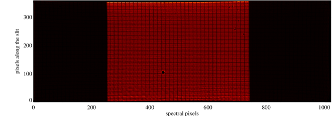
Figure 6.: Image of a grid shadow placed in close proximity of the detector during laboratory testing showing the cushion shape distortion. Note that the bright central part is caused by the photocathode coating. Dark pores are visible. The grid structure has been used to determine the deviation of the image from the ideal rectangular structure with a uniform plate scale.fig:grid

In addition to the geometric distortion, the spectral lines are inclined with respect to the detector vertical lines due to a discrepancy in the orientation of the grating and the detector. For precise wavelength measurements a highly accurate linearization of the spectral plate scale is necessary. Thus, the image distortions need a geometrical correction such that the curvature of spectral lines is removed and the wavelength scale is made linear. A combination of the laboratory images and data from cool solar emission lines acquired for this particular purpose have been used to extract the needed information for creating the geometric correction arrays (Moran, 2002). The arrays consist of lookup tables with pixel shift vectors that can be applied by using a bilinear interpolation algorithm to correct the distorted frames with a standard uncertainty of 0.11 pixel in spectral and 0.25 pixel in spatial direction. This algorithm incorporates resizing of the pixels while maintaining the radiometric accuracy. As a side effect of this treatment, empty values will be produced in some pixels near the edges. This led to an adverse effect in those cases where adjacent windows were selected, since these empty pixels may cut out important parts of the line of interest. Therefore we had to concatenate individually read out windows to produce full-size formats. These ‘inserted’ full image formats led to a significant blow up of the data volume of the archive.

The distortion correction for both detectors is based on images of a rectangular grid that was placed in front of the detector before integration. This may explain, why a residual distortion still remains for edge pixels.

4.5 Dead-Time and Local-Gain Effects

The total count rate of a detector during one exposure may be so high that individual photon events may not be detected correctly and electronic deadtime correction factors must be applied. The deadtime effect of the detector electronics is not negligible whenever the total count rate on the detector is above 50 000 s^-1. The deadtime-corr.pro routine takes care of this effect and corrects the radiometric calibration using the total count rate as input. Note that the total count rate on the detector cannot be inferred from subformat images. Instead, this information is taken from the detector housekeeping channel. Due to the cyclic readout of detector housekeeping data – a process that is asynchronous to the science observation – the actual incoming event rate may not be updated fast enough in the header data when a change of photon flux happened less a minute before the exposure.

The local count rate in a spectral line may also be high, such that the local gain in this part of the detector channel plate is reduced and pulses may fall below the detection threshold. This reduction in responsivity can be corrected by the local-gain depression correction as long as the incoming photon flux is moderate and the pixel count rate is below $\approx$20 s^-1. For higher pixel count rates, the uncertainty increases dramatically. In case of severe overexposure, the number of valid counts will be reduced instead of going up. Although the scientific use of such spectra is questionable, they appear unflagged in the archive.

5 Radiometric Calibration

sec: Radio

In this section, the radiometric calibration of the spectrometer SUMER and related aspects will be outlined. The spectroradiometry to be employed is covered in many publications that will be summarized here with reference to the most relevant original articles.

The solar electromagnetic radiation — of which SUMER can observe the wavelength range from 46.5 nm to 161.0 nm — can be characterized by the total solar irradiance (TSI) and its spectral distribution, the solar spectral irradiance (SSI), as a function of the wavelength, $\lambda$ (or, alternatively, the frequency, $\nu$). Quantitative information on these quantities can only be obtained with calibrated instrumentation, i.e. the observations must be compared to laboratory-based standards, thereby providing a baseline for short-term and long-term investigations of any solar variability (cf. Quinn and Fröhlich, 1999; Lean, 2000; Willson and Mordvinov, 2003; Wilhelm, 2009, 2010). The physical quantities have to be given in units of the International System of Units (SI: Le système international d’unités) (BIPM, 2006; see also NIST, 2008).

5.1 Calibration Concept

concept

In Table Tab_Units, some derived SI units of physical quantities are compiled that are relevant in the context of spectroradiometry.

Table 2.: Derived SI units used in spectroradiometry.

Quantity	Symbola	Unit symbol	Unit name of quantities
Radiant energy	$Q$	J	joule (1 J=1 kg m2 s-2)
Radiant flux, power	$\mathit{\Phi}$	W	watt (1 W=1 J s-1)
Spectral flux	${\mathit{\Phi}}_{\lambda}$	W nm-1
Irradiance	$E$	W m-2
Spectral irradiance	$E_{\lambda}$	W m-2 nm-1
Radiance	$L$	W m-2 sr-1
Spectral radiance	$L_{\lambda}$	W m-2 sr-1 nm-1
Radiant intensity	$I$	W sr-1
Spectral intensity	$I_{\lambda}$	W sr-1 nm-1

^a Recommendations only. Tab_Units

Four quantities are of major importance for the spectroradiometry: the “radiant flux density” or “irradiance”, $E$; the “spectral irradiance”, $E_{\lambda}$; the “radiance”, $L$; and the “spectral radiance”, $L_{\lambda}$. They are given in Table Tab_Units together with supporting explanations. Note that the radiance and the intensity are not dependent on the observing distance, whereas the irradiance varies with the inverse square of the distance. The spatially-resolved observations of SUMER yield the spectral radiance, $L_{\lambda}(\vartheta,t)$, defined by the relation

$${\rm d}Q(\lambda,\vartheta,t)=L_{\lambda}(\vartheta,t)\,{\rm cos}\vartheta\,{\rm d}S\,{\rm d}\omega\,{\rm d}t\,{\rm d}\lambda~{},\ilabel{radiance}$$ (1)

where d$Q$ is the differential radiant energy emitted into the solid angle ${\rm d}\omega$ from $\cos\vartheta\,{\rm d}S$, the projected area normal to the direction of ${\rm d}\omega$, during the time interval ($t,~{}t+{\rm d}t$) in the wavelength interval ($\lambda,~{}\lambda+{\rm d}\lambda$). An average value of the spectral radiance, $\overline{L_{\lambda}}$, over certain solid angle, time, and wavelength intervals can be obtained from a measurement of the energy

$$\mathrm{\Delta}Q~{}=~{}\overline{L_{\lambda}}\,\mathrm{\Delta}\Omega\,\mathrm{\Delta}t\,\mathrm{\Delta}\lambda\,A\ilabel{energy}$$ (2)

through the aperture area, $A$, of SUMER (cf. Wilhelm, 2002a). If the wavelength interval $\Delta\lambda$ covers the profile of a spectral line at $\lambda$, $L_{\rm line}=(\overline{L_{\lambda}}-L_{\rm back})\,\Delta\lambda$ represents — after a suitable background subtraction — its line radiance.

As mentioned before, the radiometric calibration must be traceable to laboratory standards. Ideally these would be primary standards —  absolute radiation sources that can be realized in the laboratory (Smith and Huber, 2002). Synchrotron radiation constitutes a suitable source standard in the VUV range, because the spectral radiant flux emitted can be calculated from the parameters of the electron or positron storage ring (Schwinger, 1949; Hollandt et al., 2002). In most cases, secondary standards have to be engaged as transfer standards between primary standards and the instrumentation to be calibrated, because the operational requirements of the primary standard and those of the test specimen are often not compatible.

5.2 SUMER Radiometric Calibration

radiometry

A calibration of the SUMER spectrometer designed for operation on a spacecraft directly at a synchrotron facility would have caused conflicts in cleanliness requirements and schedule constraints. A transfer standard equipped with a hollow-cathode plasma-discharge lamp was therefore calibrated with BESSY I at the PTB laboratory for 32 emission lines with wavelengths between 53.7 nm and 147.0 nm. This was done by a comparison of the radiation characteristics of both standards with the help of a VUV monochromator, taking into account the polarization of the synchrotron beam. The calibration of the transfer standard was carried out before (and after) it was used to characterize the spectral response of SUMER. During the calibration runs, a reproducibility of the radiant flux could be obtained in certain spectral lines within $\pm\,2.5\,\%$ over several hours, and $\pm\,5\,\%$ after a change of the filling gas (Hollandt et al., 1996, 1998, 2002; Wilhelm et al., 2000).

The laboratory calibration was intended to measure the radiometric response of the system, as far as mirror reflectivities and detector responsivities were concerned, without internal vignetting. Contributions to the relative standard uncertainty by the various subsystems have been compiled in Table Uncertainties for the central wavelength range. The data resulted in relative standard uncertainties of 0.11 using the 2 mm hole in place of the slit, 0.12 with the nominal slit and 0.18 for the 0.3^′′$\times$ 120^′′ slit. Based on these measurements Figures fig:cal(a) and fig:cal(b) have been plotted.

Table 3.: Contributions to the relative uncertainties (wavelength range 53.7 nm to 123.6 nm).

Item	Quantity	Uncertainty
		(1 $\sigma$)
Transfer standard	($6.80\times 10^{6}$ to $7.04\times 10^{8}$) s-1	0.06 to 0.07
(photon flux)
Detector and	5.64 mm2/(9.5 mm $\times$ 27.0 mm)a
telescope inhomogeneities	140 mm2/(90 mm $\times$ 130 mm)a	0.08
Aperture stop	90 mm $\times$ 130 mm	0.001/0.001
Focal length of telescope	1302.77 mm at 75 ∘C	$5\times 10^{-5}$
Slits:
#1 (4′′$\times$ 300′′)	26.03 $\mu$m $\times$ 1889.7 $\mu$m	0.005/0.003
#2 (1′′$\times$ 300′′; nominal)	6.23 $\mu$m $\times$ 1889.7 $\mu$m	0.016/0.003
#4 (1′′$\times$ 120′′)b	6.27 $\mu$m $\times$ 755.4 $\mu$m	0.016/0.005
#7 (0.3′′$\times$ 120′′)b	1.76 $\mu$m $\times$ 755.4 $\mu$m	0.045/0.005
#9 ($\oslash$: 317′′; calibration)	2 mm diameter hole	0.003
Nominal/calibration slit	0.0110 (signal ratio)	0.05
Lyot stop	27.73 mm $\times$ 40.12 mm	0.004/0.003
Slit diffraction	Model calculations	0.01
Detector pixel size (mean)	26.5 $\mu$m (spat.)$\times$ 26.5 $\mu$m (spectr.)	0.02/0.015
Detector	Flatfield and distortion corrections	0.01
a. Illuminated area during calibration at any time divided by total size of optically effective area.
b. Slits #3 (6) and 5 (8) are identical with slit #4 (7), but offset in spatial direction. The extreme
pixels of slits #5 and #8 are vignetted.

Uncertainties

The scattered-light measurements were carried out using a source emitting two intense Kr i lines at 116.5 nm and 123.6 nm, because they have wavelengths close to the bright H i Ly-$\alpha$ line at 121.6 nm. The laboratory results showed excellent stray-light characteristics. Nevertheless, the scattered light of the H i Lyman-$\alpha$ and $\beta$ lines could be observed at 1700^′′ from the centre of the solar disk in order to obtain line profiles unaffected by the geocorona (Lemaire et al., 1998, Lemaire 2002; Emerich et al., 2005).

5.3 Calibration Tracking

tracking

A critical issue is the stability of the spectroscopic responsivity, which can be affected by obstructions of the apertures or contamination of the optical elements and detectors. Solar ultraviolet radiation leads to photo-activated polymerization of contaminating hydrocarbons and, as a result, to a permanent degradation of the system. A cleanliness programme is therefore of great importance to ensure particulate and molecular cleanliness of the instruments and the spacecraft (Schühle, 1993, 2003; Thomas, 2002). An instrument door and an electrostatic solar wind deflector in front of the primary telescope mirror are specific features incorporated in the design in order to maintain the radiometric responsivity during launch and the operational phases.

Nevertheless it is essential to track the calibration status through all phases of the mission, i.e., transport, spacecraft integration and tests, launch, commissioning as well as operations. The procedures include in-flight calibration using line ratios provided in atomic physics data (Doschek et al., 1999; Landi et al., 2002), inter-calibration between instruments (Wilhelm, 2002b), degradation monitoring (Wilhelm et al., 1997; Schühle et al., 1998, 2000a):

1. In order to obtain a radiometric characterization outside the spectral range covered in the laboratory, line-radiance ratios measured on the solar disk have been compared with the results of atomic physics calculations.

2. A deep-exposure reference spectrum obtained with detector A in a stable coronal streamer on 13 and 14 June 2000 showed the Si xii pair at 49.94 nm and 52.07 nm in second and third order of diffraction. This allows us to establish responsivity curves in third order for both photocathodes.

3. Integration of the spectral radiance using full-disk SUMER scans have been performed in the N v line at 123.8 nm and the C iv line at 154.8 nm in 1996. The spectral irradiance of the Sun so obtained could be compared with the Solar Stellar Irradiance Comparison Experiment on the Upper Atmosphere Research Satellite (SOLSTICE/UARS; Rottman et al., 1993; Woods et al., 1993) radiometrically calibrated at the Synchrotron Ultraviolet Radiation Facility (SURF-II) at NIST. Agreement within a factor of 1.14 was found for the N v line and approximately 1.10 for the C iv line (Wilhelm et al., 1999).

4. Stellar observations (Lemaire, 2002) and reference spectra of QS regions taken on both detectors indicated that the data points available for both detectors are not systematically different within the relative uncertainty margin of $\pm 20$ %. It was thus possible to determine joint KBr responsivity functions for detectors A and B in Figure fig:cal(b).

5. A stable radiometric calibration is also supported by the results of the flatfield exposures performed in the H i Lyman continuum near 88 nm in QS areas. No significant change of the responsivity of detector A has been found over 200 days, nor was there any decrease in detector B over 350 days (Schühle et al., 1998).

6. However, a major change of the responsivity happened during the attitude loss of SOHO in 1998. After the recovery, a responsivity decrease was found over a wide spectral range as shown in Figures fig:cal(c) and fig:cal(d). This change is attributed to the deposition of contaminants and subsequent polymerization on the optical surfaces of the instrument, because both detectors were equally affected. Relative losses of 26 % for He i 58.4 nm, 28 % for Mg x (60.9 and 62.4) nm, 34 % for Ne viii 77.0 nm, 39 % for N v 123.8 nm, and 29 % for the H i Lyman continuum were obtained, resulting in an average relative loss of 31 % (Schühle et al., 2000b). Star observations of $\alpha$ Leonis before and after the attitude loss provide strong evidence that the responsivity decrease is wavelength dependent with a tendency to become rather small at the longest wavelengths (Lemaire, 2002). Consequently, we adopted a relative loss in the responsivities of 31 % for wavelengths shorter than 123.8 nm (N v) (as before), which linearly decreases to 5 % at 161 nm.

Figure 7.: Spectral responsivities of the SUMER instrument with its detectors A and B, and the corresponding relative uncertainties for the nominal slit. (a) In the upper panel the responsivity ratio of the photocathodes is shown. (b) First-order and second-order KBr responsivities evaluated jointly for both detectors. The long-wavelength deviation of detector B is treated in the text as well as the bare MCP responsivities and the third-order calibration. Independent assessments of (c) detector A and (d) detector B. For both detectors the relative uncertainties inside and outside the wavelength band from 53.7 nm to 123.6 nm and their changes after the recovery of SOHO are indicated. (On the long-wavelength side, the relative uncertainty refers to the KBr photocathode only.) fig:cal

The responsivities of SUMER are shown in Figure fig:cal as a typical result of the ground and in-flight calibration activities. Note that the radiant energy is measured here as the number of photons with energy $h\,\nu=h\,c_{0}/\lambda$, where $h$ is Planck’s constant and $c_{0}$ the speed of light in vacuum. This convention is often adopted in radiometry. The spectral responsivity curves displayed in Figure fig:cal refer to situations with low count rates both for the total detector and for single pixels. Whenever the total count rate exceeds about $5\times 10^{4}$ s^-1, a deadtime correction is required; and with a single-pixel rate above about 3 s^-1, a gain-depression correction is called for (see Section 3.4). The uncertainties given in panels (c) and (d) include the contributions of optical stops and diffraction effects, but the uncertainty of the pixel size has to be treated separately. When applying spectral responsivity curves as shown in Figure fig:cal(b), (c) and (d) to the telemetry data, it is necessary to take into account the effects of field stops as well as the epoch of the observation. This can be accomplished by applying the SUMER calibration programme radiometry.pro . The programme can perform all calculations in photon units or in energy units in accordance with SI. As an example, Figure fig:spec depicts the VUV radiance spectrum of a QS region with many emission lines and some continua in the wavelength range from 80 nm to 150 nm.

Figure 8.: Spectral radiance of the quiet Sun in the VUV range from a region near the centre of the disk. Prominent emission lines are marked. The spectral radiances expected for some brightness temperatures, $T_{\rm B}$, are shown in red as approximations of the continua in the corresponding wavelength ranges (after Wilhelm and Fröhlich 2010).fig:spec

The responsivity curves are available for the periods from January 1996 to June 1998 and from November 1998 to December 2001. They have undergone modifications in the past and might do so again in the future. There are two reasons for such modifications: an improved understanding of the performance of the instrument including its calibration; and changes of the status of the instrument with time. There are indications that the responsivity of the instrument did not change at least until April 2007, although the uncertainties increased. After April 2010, however, a thermal runaway effect in the MCP of detector B forced us to reduce the high voltage. This resulted in a significant drop of the sensitivity and a partial loss of the KBr coated section of the detector. Since April 2012, only the bare sections of detector B can be used. Figure 10.2 of Wilhelm et al.(2002) summarizes the modifications since October 1999 continuing the history documented in Figure 4 of Wilhelm et al.(2000), demonstrating that the calibration status in the central wavelength range is very consistent over time for both detectors. We recommend in general the joint evaluation, but near 80 nm both detectors cannot be treated jointly. Thus the separate responsivity of detector B should be used here. Before an adequate low-gain level of detector B was found, a test configuration was used between 24 September and 6 October 1996.

5.4 Other Data Reduction Aspects

Various other data correction algorithms have been established that are used for special applications, but have not been included in the set of standard data reduction procedures applied to the data in the archive.

5.4.1 Wavelength Calibration, Line Identification, Doppler Velocities

sec: Doppler

The wavelength setting is accomplished by the linear movement of a rod that changes the reflection angle of the plane mirror and thus the angle of incidence on the grating (cf., Section 2.2.3). The relationship between actuator step and wavelength setting is highly non-linear and has been approximated by a lookup table. This lookup table and the dispersion relation as discussed before have been used to convert the spectral pixels to physical units. The wavelength of L1 data is given in unit of nanometer. The limited accuracy and reproducibility of the wavelength setting introduce an uncertainty of several pixels, which is far below the spectral resolution. A more careful wavelength calibration is required, if it is important to know the absolute wavelength of a spectral line. Since SUMER has no on-board calibration lamp, each set of spectra with the same wavelength setting has in this case to be calibrated using nearby photospheric and chromospheric lines of the solar spectrum as wavelength standards. This cannot be completed in an automated manner and will be the task of the user. The wavelength calibration in the archive is based on the nominal dispersion. Moreover, it assumes that the line of interest is at the central pixel of the spectral window. Unpredictable offsets of many pixels render this assumption as unrealistic. Therefore, the automated wavelength scale given in the archive is only a first guess.

Even very faint lines could be detected in deeply exposed on-disk and off-disk spectra because of the extremely low level of dark counts, and many new line identifications were possible. A comprehensive overview of the solar spectrum in the SUMER spectral range is provided in spectral atlases of disk (Curdt et al., 2001) and coronal features (Curdt et al., 2004).

Centroiding allows to determine the position of unblended spectral lines down to one tenth of a pixel, in particular for lines observed in second order of diffraction. The line shift $\delta\lambda$ can be used to calculate the Doppler flow $v_{\rm D}$ using

$$v_{\rm D}=\frac{\delta\lambda}{\lambda}\,c_{0}$$ (3)

where $c_{0}$ is the speed of light in vacuum and $\lambda$ the wavelength of the spectral line. Several conditions must be met to reach uncertainties as low as 1 km s^-1 to 2 km s^-1: the line of interest must be unblended and gaussian; its laboratory wavelength must be well-known; and wavelength standards have to be at rest and close to the line of interest.

The limiting parameter for the effective spectral resolution of the instrument is certainly given by the detector non-linearity and instability.

5.4.2 Pixel Shift

sec: Deltapixel

The location of the slit image on the detector array is not at all constant. The size of the slit image varies with wavelength – an effect of the wavelength-dependent magnification (cf., Section 2.1). The accumulated effect of the alignment errors between the scan mirror rotation axis, the grating ruling direction, the direction of the grating focussing mechanism, and the direction of the detector rows can be evaluated for the distortion-corrected detector arrays (both A and B) by the function deltapixel.pro as shown in Table tab:shift. The correction for this pixel shift is only needed for co-registration of spectra with different wavelength settings. For such cases, numerical values can be extracted from the lookup table in Table tab:shift. There is no compensation for this effect in the data of the archive.

Table 4.: Lookup table. Nominal position of upper and lower pixels of the 120^′′ slit at different wavelengths for detector B data (for detector A the wavelengths are offset by $\approx$12.0 nm to higher values). The shift is given relative to the slit image at a wavelength setting of 115.2 nm. The shift values are basically negative which corresponds to an apparent offset towards the North in SUMER coordinates.tab:shift

Wavelength	Lower	Upper	Pixel	Wavelength	Lower	Upper	Pixel
$\lambda$ / nm	pixel	pixel	shift	$\lambda$ / nm	pixel	pixel	shift
69.2	105.6	220.9	-16.8	109.2	119.5	238.7	-0.9
71.2	106.5	222.1	-15.7	111.2	119.8	239.2	-0.5
73.2	107.4	223.2	-14.7	113.2	119.9	239.7	-0.2
75.2	108.2	224.1	-13.8	115.2	120.0	240.0	0.0
77.2	109.0	225.1	-13.0	117.2	119.3	240.2	0.1
79.2	109.7	226.0	-12.1	119.2	119.7	240.3	0.0
81.2	110.5	226.8	-11.3	121.2	119.4	240.2	-0.2
83.2	111.2	227.7	-10.5	123.2	118.9	239.9	-0.6
85.2	112.0	228.6	-9.7	125.2	118.2	239.5	-1.1
87.2	112.7	229.5	-8.9	127.2	117.4	238.9	-1.9
89.2	113.5	230.3	-8.1	129.2	116.4	238.1	-2.8
91.2	114.2	231.2	-7.3	131.2	115.2	237.1	-3.9
93.2	114.9	232.1	-6.5	133.2	113.8	235.9	-5.1
95.2	115.6	233.0	-5.7	135.2	112.3	234.5	-6.6
97.2	116.3	233.9	-4.9	137.2	110.5	232.9	-8.3
99.2	117.0	234.8	-4.1	139.2	108.6	231.1	-10.1
101.2	117.6	235.7	-3.4	141.2	106.5	229.2	-12.1
103.2	118.2	236.5	-2.7	143.2	104.3	227.1	-14.3
105.2	118.7	237.3	-2.0	145.2	101.8	224.9	-16.7
107.2	119.1	238.0	-1.4	147.2	99.3	222.5	-19.1

5.4.3 Line Broadening

sec: linewidth

The width of spectral lines is affected by a contribution of the instrumental broadening to the Doppler broadening. Using the function con-width-funct-3.pro the instrumental width can be taken out by using a de-convolution matrix.

5.4.4 Straylight and Dark Signal

sec: Straylight

Because of the excellent surface quality of the primary mirror (cf., Section 2.1; ‘Optical design’), the scattered light of the disk falls off by five orders of magnitude within 20 arcsec (cf., Figure 1 in Lemaire et al., 1998). It is, therefore, possible to observe the lower corona off-disk without occultation. At larger limb distances, however, the off-limb scattered light dominates the spectra. The fall-off curves for the scattered light levels are the result of the large-angle scatter characteristic of the micro-roughness of the mirror coating, which is wavelength dependent and also depends on the non-uniform and variable brightness distribution of the disk. It is therefore not possible to apply an easy algorithm for automatic straylight subtraction. For many applications, the scattered light is unproblematic, it may even help with the wavelength calibration. In all other cases the straylight has to be subtracted by the user.

During the first years in orbit, the data from the photon counting detection system was practically noise-free (cf., Section 2.3 or Wilhem et al., 1997a). Only during rare solar energetic particle (SEP) events with a strong high energy contribution a temporary increase of dark counts was observed. The rate of dark counts increased, however over the years, and recently, the number of flaring pixels may become a problem for long exposures at low signal.

5.4.5 Thermo-Elastic Deformation Effects

An analysis by Rybák et al. (1999) revealed a parasitic effect of the algorithm used to regulate the temperature of the optical bench. It was found that the oscillation of the heater duty cycle had an effect of the line position on the detector due to thermoelastic deformations. For the front section of the instrument, Rybák et al. (1999) report oscillation amplitudes of $\approx$0.3 K with a period of $\approx$120 min. Similarly, in the rear section of the instrument the temperature oscillates with an amplitude of $\approx$0.1 K and with a period of $\approx$75 min. As a consequence of these temperature variations, the position of a spectral line was periodically shifted by up to 2.5 nm, dominated by the front bench. Rybák et al. (1999) also report a correction procedure needed for long-duration studies during the first years that are sensitive to this effect.

With increasing equilibrium bulk temperatures (ageing effect of the thermo- optical properties), the need of the heaters was reduced and the heater duty cycle diminished. Already in 1998, the thermoelastic deformations became very small and disappeared later.

6 Archive Description

sec: Archive

Figure fig:dataflow shows the path from the various data sources towards the SUMER FITS data products, including intermediate processing steps.

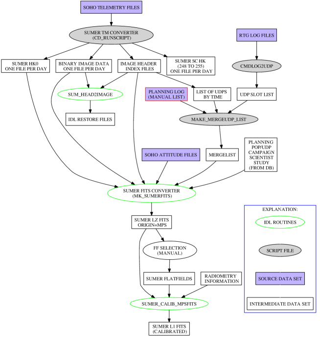
Figure 9.: Data Flow Diagram.fig:dataflow

6.1 FITS LZ

sec: fitslz The IDL routine mk_sumerfits takes the binary data from the TM processing (see Section sec: TM processing) and produces SUMER LZ FITS data. The main task is to create a FITS header with all the information needed. In addition some missing HK0 data is correlated to the image (see Section sec: HK). This routine takes care of assembling several wavelength windows taken with one exposure into one detector image (see Table tab:formats). This step is necessary because of the difficulty that further processing steps like geometrical correction ‘deform’ the image so that a composition of two adjacent images will not be possible without gaps.

The SUMER FITS LZ product is decompressed, solar coordinate corrected (North up) and wavelength direction corrected (low to high from left to right) data. All further processing steps described in Section sec: Intro are performed in the FITS L1 processing which is described in Section sec: fitsl1.

6.1.1 LZ FITS File Structure

sec: fitslzfile The created SUMER LZ FITS file contains a Header Data Unit - the header, and a Primary Data Unit - the image data. In addition there is an extension.

• This is the primary FITS header (an example is given in the electronic supplementary material).

• This is the actual image data set.

• The original telemetry image header(s) of the image. This is a byte array of at least 120 bytes which can be analysed with the SUMER header routines (see the SUMER Data Cookbook for details). This data is kept for compatibility so that the ‘old’ routines can also be used to analyse the data. For each image acquired during the detector integration (1 to 8), there is one 120 byte array.

6.2 FITS L1 - Calibrated Data

sec: fitsl1

6.2.1 Definition

The SUMER FITS L1 data is defined calibrated data, where all processing steps described in Section sec: Intro are performed including radiometric calibration.

6.2.2 Restrictions

The calibration of SUMER data is only possible for data compressed with the SUMER lossless compression schemes 6 and below (see SUMER Operations Guide). Images compressed with other schemes and from the rear slit camera are ignored by the L1 processing.

6.2.3 Flatfields

sec: fitsflatfield Before starting to describe the production of the calibrated SUMER FITS data (L1) a short description is given for the preparation of the flatfield data out of the newly created SUMER FITS LZ data.

During the processing of SUMER LZ data images matching the conditions for SUMER flatfields are logged with their filename in a list. This list is afterwards taken to produce the flatfield data for the L1 production process. The IDL routine sum_make_fits_ff takes care of all the necessary steps. One of these steps is to remove the odd-even pattern from the raw image (see Section sec: FF).

Another step results from the changed acquisition strategy in later times of SUMER operation. In the beginning a flatfield was taken as one long exposure and then processed and stored for on-board flatfielding. These data were downlinked as two separate images, one was the raw data and one the processed on-board flatfield. Later, due to the ‘odd-even pattern’ (see Section sec: FF, the on-board processing was skipped and only the raw data were downlinked. To exclude transmission errors of the flatfield, the flatfield was taken in several single exposures which were then added to one flatfield image. This addition is also done by sum_make_fits_ff.

In addition this routine ‘corrects’ some image rows which were missing due to telemetry gaps. The replacement is indicated in the FITS header, as a comment.

6.2.4 Processing

sec: L1Processing

The L1 processing takes LZ data sets and performs all necessary processing to get the calibrated data. The overall routine proc_sumer_calib takes care of the in and outfile organization e.g. reading LZ files and putting all processed data into a new file.

All the calibration steps are included in the routine sumer_calib_mpsfits which is called by proc_sumer_calib. This routine calls the various SUMER calibration routines in the correct order and logs the performed processing in the FITS header.

Via parameters, the processing level can be controlled to do a step-by-step calibration for verification.

Reverse Flatfield

If an on-board faltfield processing has already been done, this is reversed for preparation of the odd-even correction.
The FITS keywords reflecting this processing are:

Keyword	Description
SSFF	Mark as not processed on board
RFLATFIL	Used reverse flatfield
history	Applied sum_flatfield (reverse)

Dead Time Correction

The dead time correction step is performed by the deadtime_corr routine.
The FITS keywords reflecting this processing are:

Keyword	Description
DEADCORR	Dead time correction
DCXDLEV	Dead time corr XDL input value
history	Applied deadtime_corr

Odd Even Correction

The odd even correction is performed by the sum_flatfield giving the oddeven array for the specified detector as a parameter.
The FITS keywords reflecting this processing are:

Keyword	Description
ODEVCORR	Odd-even correction
history	Applied sum_flatfield with odd-even corr

Local Gain Correction

Local gain correction is performed by calling the subroutine local_gain_corr.
The FITS keywords reflecting this processing are:

Keyword	Description
LGAINCOR	Local gain correction
history	Applied local_gain_corr

Flatfield Correction

The flatfield used is the one closest in time ahead of the image acquisition date. The processing itself is done by the function sum_flatfield using the image and the flatfield data as parameters.
The FITS keywords reflecting this processing are:

Keyword	Description
FLATCORR	Record the processing
FLATFILE	Used flatfield data
history	Applied sum_flatfield

Distortion Correction

Distortion correction for the data is done by calling the function destr_bilin with the image data as parameter.
The FITS keywords reflecting this processing are:

Keyword	Description
GEOMCORR	Record the processing
history	Applied destr_bilin

Radiometric Calibration

The radiometric calibration is performed by calling the s_fitsrad subroutine. This routine takes care of the calculation of the different radiometries (first or second order, KBr or bare) by calling the radiometry function with the appropriate parameters. Once the radiometry values for first and second order are calculated, the first order radiometry is applied to the image data. Both radiometry arrays are then stored in the FITS file as an extension.
The FITS keywords reflecting this processing are:

Keyword	Description
RADCORR	Radiometry calibration performed
RADORDER	Radiometry for wavelength order (first or second order)
AVARADO	Available radiometry orders
IMGUNITS	Units for image (W sr-1 m-2 Å-1)
LEVEL	1
PRODLVL	L1
history	Applied radiometry

L1 FITS File Structure

After having done all the calibration steps and gathered all needed data the data is written back to the FITS file in the following order:

• This is the primary FITS header (an example is given in the electronic supplementary material).

• This is the actual calibrated image data set.

• (cf., Section sec: fitslzfile

• This extension includes the radiometry arrays for first and second order. Since only one radiometric calibration can be performed on the data at a time, the purpose of this data arrays is to be able to reverse the actual radiometric calibration (indicated in keyword RADORDER) and perform the other one - if available. The number of available orders/arrays is indicated in the keyword AVARADO.

6.3 Processing Remarks

The IDL routines used for the FITS creation and calibration processing check on various FITS keywords for processing conditions and if processing can be performed on the specified data set. The routines also record performed processing steps in FITS keywords, so a processing step can not accidently be performed twice on the data.

7 Conclusion

Scientists all over the world who have been using SUMER data have, sharing their experience, contributed to this work (cf., Figure fig:publ). The benefits of this long learning process are comprised in the SUMER archive. Here, we have made an effort to describe the non-trivial task of processing these data in great detail and in a transparent manner. The trend in Figure fig:publ clearly indicates that there is still interest in SUMER data and that it is realistic to assume that future work will come. It is our intention to encourage future users to take advantage of such ready-to-use data that is not dependant on computer systems. SUMER is now close to end of the operational life time. Therefore, in the future the archive will – with the exception of Interface Region Imaging Spectrograph (IRIS; dePontieu et al.., 2012) spectra – be the only source of data in the SUMER spectral range. We tried hard to complete the archive so that it can be used for joint science with IRIS. And we hope that in this new format enough meta information is provided that can be used for data mining.

The SUMER project is financially supported by DLR, CNES, NASA, and the ESA PRODEX Programme (Swiss contribution). SUMER is part of SOHO of ESA and NASA. The instrument was jointly operated by teams from IAS and MPS. We specially thank Gilles Poulleau servicing the ground equipment for so many years. Numerous scientists of the community helped to coordinate the science operations.

References

- BIPM (2006) Bureau International des Poids et Mesures (BIPM): 2006, Le système international d’unités (SI), 8e éd, Sèvres, France.
- Curdt et al. (2001) Curdt, W., Brekke, P., Feldman, U., Wilhelm, K., Dwivedi, B.N., Schühle, U., Lemaire, P.: 2001, The SUMER spectral atlas of solar disk features. A&A 375, 591–613.
- Curdt et al. (2004) Curdt, W., Landi, E., Feldman, U.: 2004, The SUMER spectral atlas of solar coronal features. A&A 427, 1045–1054.
- Delaboudinière et al. (1995) Delaboudinière, J.-P., Artzner, G.E., Brunaud, J., Gabriel, A.H., Hochedez, J.F., Millier, F., et al.: 1995, EIT: Extreme-Ultraviolet Imaging Telescope for the SOHO mission. Sol. Phys. 162, 291–312.
- Doschek et al. (1999) Doschek, E.E., Laming, J.M., Doschek, G.A., Feldman, U., Wilhelm, K.: 1999, A comparison of measurements of solar extreme-ultraviolet spectral line intensities emitted by C, N, O, and S ions with theoretical calculations. ApJ 518, 909–917.
- Emerich et al. (2005) Emerich, C., Lemaire, P., Vial, J.-C., Curdt, W., Schühle, U., Wilhelm, K.: 2005, A new relation between the central spectral solar H i Lyman irradiance and the line irradiance measured by SUMER/SOHO during the cycle 23. Icarus 178, 429–433.
- Feldman et al. (2000) Feldman, U., Curdt, W., Landi, E., Wilhelm, K.: 2000, Identification of spectral lines in the 500-1600 Å wavelength range of highly ionized Ne, Na, Mg, Ar, K, Ca, Ti, Cr, Mn, Fe, Co, and Ni emitted by flares. A&A 544, 508–521.
- Hollandt et al. (1996) Hollandt, J., Schühle, U., Paustian, W., Curdt, W., Kühne, M., Wende, B., Wilhelm, K.: 1996, Radiometric calibration of the telescope and ultraviolet spectrometer SUMER on SOHO. Appl. Opt. 35, 5125–5133.
- Hollandt et al. (1998) Hollandt, J., Schühle, U., Curdt, W., Dammasch, I.E., Lemaire, P., Wilhelm, K.: 1998, Solar radiometry with the telescope and vacuum-ultraviolet spectrometer SUMER on the solar and heliospheric observatory (SOHO). Metrologia 35, 671–675.
- Hollandt et al. (2002) Hollandt, J., Kühne, M., Huber, M.C.E., Wende, B.: 2002, Source standards for the radiometric calibration of astronomical instruments in the VUV spectral range traceable to the primary standard BESSY. In: Pauluhn, A., Huber, M.C.E., von Steiger, R. (eds.), The Radiometric Calibration of SOHO, ESA SR-002, 51–68.
- Landi et al. (2002) Landi, E., Feldman, U., Dere, K.P.: 2002, CHIANTI – An atomic database for emission lines. V. Comparison with an isothermal spectrum observed with SUMER. Astrophys. J. Suppl. 139, 281–296.
- Lean (2000) Lean, J.: 2000, Evolution of the Sun’s spectral irradiance since the Maunder Minimum. Geophys. Res. Lett. 27, 2425-2428.
- Lemaire (2002) Lemaire, P.: 2002, SUMER stellar observations to monitor responsivity variations. In: Pauluhn, A., Huber, M.C.E., von Steiger, R. (eds.), The Radiometric Calibration of SOHO, ESA SR-002, 265–270.
- Lemaire et al. (1997) Lemaire, P., Wilhelm, K., Curdt, W., Schühle, U., Marsch, E., Poland, A.P., et al.: 1997, First results of the SUMER telescope and spectrometer on SOHO. II. Imagery and data management. Sol. Phys. 170, 105–122.
- Lemaire et al. (1998) Lemaire, P., Emerich, C., Curdt, W., Schühle, U., Wilhelm, K.: 1998, Solar H i Lyman full disk profile obtained with the SUMER/SOHO spectrometer. A&A 334, 1095–1098.
- Lemaire et al. (2002b) Lemaire, P., Emerich, C., Vial, J.-C., Curdt, W., Schühle, U., Wilhelm, K.: 2002, Variation of the full Sun hydrogen Lyman and profiles with the activity cycle. In: Wilson, A. (ed.), SOHO 11-Symposium on From Solar Min to Max: Half a Solar Cycle with SOHO, ESA SP-508, 219–222.
- Moran (2002) Moran, T.G.: 2002, Solar and Heliospheric Observatory/Solar Ultraviolet Measurements of Estimated Radiation ultraviolet array detector distortion correction. Rev. Sci. Instrum. 73 3982–3887.
- NIST (2008) National Institute of Standards and Technology (NIST): 2008, Guide for the Use of the International System of Units (SI), NIST Special Publication 811.
- Quinn and Fröhlich (1999) Quinn, T.J., Fröhlich, C.: 1999, Accurate radiometers should measure the output of the Sun. Nature 401, 841.
- Rottman et al. (1993) Rottman, G.J., Woods, T.N., Sparn, T.P.: 1993, Solar-Stellar Irradiance Comparison Experiment 1. 1. Instrument design and operation. J. Geophys. Res. 98, 10667–10677.
- Rybák et al. (1999) Rybák, J., Curdt, W., Kucera, A., Schühle, U., Wöhl, H.: 1999, Chromosperic and transition region dynamics - Reasons and consequences of the long period instrumental periodicities of SUMER/SOHO. In: Wilson, A. (ed.), Proc. 9th European Meeting on Solar Physics. Magnetic Fields and Solar Processes. ESA SP-448, 361–366.
- Saha and Leviton (1993) Saha, T.T., Leviton, D.B.: 1993, Theoretical and measured encircled energy and wide-angle scatter of SUMER demonstration telescope mirror in FUV. In: Bely, P.Y., Breckinridge, J.B. (eds.), Space Astronomical Telescopes and Instruments II. Proc. SPIE 1945, 398–409.
- Siegmund et al. (1994) Siegmund, O.H., Stock, J.M., Marsh, D.R., Gummin, M.A., Raffanti, R., Hull, J., et al.: 1994, Delay-line detectors for the UVCS and SUMER instruments on the SOHO Satellite. In: Siegmund, O.H., Vallerga, J.V. (eds.), EUV, X-ray, and Gamma-Ray Instrumentation for Astronomie V. Proc. SPIE, 2280, 89–100.
- Smith and Huber (2002) Smith, P.L., Huber, M.C.E.: 2002, Spectroradiometry for solar physics in space. In: Pauluhn, A., Huber, M.C.E., von Steiger, R. (eds.), The Radiometric Calibration of SOHO, ESA SR-002, 21–36.
- Schühle (2003) Schühle, U.: 2003, Cleanliness and calibration stability of UV instruments on SOHO. In: Keil, S.L., Avakyan, S.V. (eds.), Innovative Telescopes and Instrumentation for Solar Astrophysics, Proc SPIE 4853, 88-97.
- Schühle (1993) Schühle, U.: 1993, The cleanliness control program for SUMER/SOHO. In: Silver, E.H., Kahn, S.M. (eds.), UV and X-Ray Spectroscopy of Astrophysical and Laboratory Plasmas., Cambridge University Press, Cambridge, 373–382.
- Schühle et al. (1998) Schühle, U., Brekke, P., Curdt, W., Hollandt, J., Lemaire, P., Wilhelm, K.: 1998, Radiometric calibration tracking of the vacuum-ultraviolet spectrometer SUMER during the first year of the SOHO mission. Appl. Opt. 37, 2646–2652.
- Schühle et al. (2002a) Schühle, U., Curdt, W., Hollandt, J., Feldman, U., Lemaire, P., Wilhelm, K.: 2000a, Radiometric calibration of the vacuum-ultraviolet spectrograph SUMER on the SOHO spacecraft with the B detector. Appl. Opt. 39, 418–425.
- Schühle et al. (2002b) Schühle, U., Hollandt, J., Pauluhn, A., Wilhelm, K.: 2000b, Mid-term radiance variation of far-ultraviolet emission lines from quiet-Sun areas. In: Wilson, A. (ed.), Proc. 1st Solar and Space Weather Euroconference. The Solar Cycle and Terrestrial Climate, ESA SP-463, 427–430.
- Schwinger (1949) Schwinger, J.: 1949, On the classical radiation of accelerated electrons. Phys. Rev. 75, 1912–1925.
- Thomas (2002) Thomas, R.: 2002, 20:20 vision and SOHO cleanliness. In: Pauluhn, A., Huber, M.C.E., von Steiger, R. (eds.), The Radiometric Calibration of SOHO, ESA SR-002, 91–104.
- Wilhelm (2002a) Wilhelm, K.: 2002a, Spectroradiometry of spatially-resolved solar plasma structures. In: Pauluhn, A., Huber, M.C.E., von Steiger, R. (eds.), The Radiometric Calibration of SOHO, ESA SR-002, 37–50.
- Wilhelm (2002b) Wilhelm, K.: 2002b, Calibration and intercalibration of SOHO’s vacuum-ultraviolet instrumentaion. In: Pauluhn, A., Huber, M.C.E., von Steiger, R. (eds.), The Radiometric Calibration of SOHO, ESA SR-002, 69–90.
- Wilhelm (2009) Wilhelm, K.: 2009, Solar energy spectrum. In: Trümper, J. (ed.), Landolt-Börnstein Database VI. Astronomy and Astrophysics, 4B The Solar System, Springer, Berlin, 10–20.
- Wilhelm (2010) Wilhelm, K.: 2010, Quantitative solar spectroscopy. Astron. Nachr. 331, 502–518.
- Wilhelm et al. (1995) Wilhelm, K., Curdt, W., Marsch, E., Schühle, U., Lemaire, P., Gabriel, A.H., et al.: 1995, SUMER – Solar Ultraviolet Measurements of Emitted Radiation. Sol. Phys. 162, 189–231.
- Wilhelm et al. (1997a) Wilhelm, K., Lemaire, P., Curdt, W., Schühle, U., Marsch, E., Poland, A.P., et al.: 1997a, First results of the SUMER telescope and spectrometer on SOHO. I. Spectra and spectroradiometry. Sol. Phys. 170, 75–104.
- Wilhelm et al. (1997b) Wilhelm, K., Lemaire, P., Feldman, U., Hollandt, J., Schühle, U., Curdt, W.: 1997b, Radiometric calibration of SUMER: Refinement of the laboratory results under operational conditions on SOHO. Appl. Opt. 36, 6416–6422.
- Wilhelm et al. (1999) Wilhelm, K., Woods, T.N., Schühle, U., Curdt, W., Lemaire, P., Rottman, G.J.: 1999, The solar ultraviolet spectrum from 1200 Å to 1560 Å: A radiometric comparison between SUMER/SOHO and SOLSTICE/UARS. A&A 352, 321–326.
- Wilhelm et al. (2000) Wilhelm, K., Schühle, U., Curdt, W., Dammasch, I.E., Hollandt, J., Lemaire, P., Huber, M.C.E.: 2000, Solar spectroradiometry with the telescope and spectrograph SUMER on the solar and heliospheric observatory SOHO. Metrologia 37, 393–398.
- Wilhelm et al. (2002) Wilhelm, K., Schühle, U., Curdt, W., Dammasch, I.E., Hollandt, J., Lemaire, P., Huber, M.C.E.: 2002, Solar vacuum-ultraviolet radiometry with SUMER. In: Pauluhn, A., Huber, M.C.E., von Steiger, R. (eds.), The Radiometric Calibration of SOHO, ESA SR-002, 145–160.
- Wilhelm et al. (2004) Wilhelm, K., Dwivedi, B.N., Marsch, E., Feldman, U.: 2004, Observations of the Sun at Vacuum-Ultraviolet Wavelengths from Space. Part I: Concepts and Instrumentation. Space Sci. Rev. 111, 415–480.
- Wilhelm et al. (2007) Wilhelm, K., Marsch, E., Dwivedi, B.N., Feldman, U.: 2007, Observations of the Sun at vacuum-ultraviolet wavelengths from space. Part II: Results and Interpretations. Space Sci. Rev. 133, 103–179.
- Wilhelm and Fröhlich (2010) Wilhelm, K., and Fröhlich, C.: 2010, Photons—from source to detector. In Huber, M.C.E., Pauluhn, A., Culhane, J.L., Timothy, J.G., Wilhelm, K., Zehnder, A. (eds.) Observing Photons in Space, ESA SR-009, 23–54.
- Wilkinson et al. (2001) Wilkinson, E., Penton, S.V., B’eland, S., Vallerga, J.V., McPhate, J., Sahnow, D.: 2001, Algorithms for correcting geometric distortions in delay lines anodes. In: Siegmund, O.H., Fineschi, S., Gummin, M.A. (eds.), UV/EUV and Visible Space Instrumentation for Astronomy and Solar Physics, Proc. SPIE, 4498, 267–274.
- Willson and Mordvinov (2003) Willson, R.C., Mordvinov, A.V.: 2003, Secular total solar irradiance trend during solar cycles 21-23. Geophys. Res. Lett. 30, 1199–1203.
- Woods et al. (1993) Woods, T.N., Rottman, G.J., Ucker, G.J.: 1993, Solar-Stellar Irradiance Comparison Experiment 1. II – Instrument calibrations. J. Geophys. Res. 98, 10 679–10 694.
- Wülser et al. (2012) Wülser, J.-P., Title, A.M., Lemen, J.R., De Pontieu, B., Kankelborg, C.C., Tarbell, T., et al.: 2012, The interface region imaging spectrograph for the IRIS Small Explorer mission. In: Space Telescopes and Instrumentation 2012: Ultraviolet to Gamma Ray, Proc. SPIE, 8443, 801–810.