The Unusual Kuiper Belt Object 2003 SQ₃₁₇

Abstract

We report photometric observations of Kuiper belt object 2003 SQ₃₁₇ obtained between 2011 August 21 and 2011 November 1 at the 3.58 m New Technology Telescope, La Silla. We obtained a rotational lightcurve for 2003 SQ₃₁₇ with a large peak-to-peak photometric range, $\Delta m=0.85\pm 0.05$ mag, and a periodicity, $P=7.210\pm 0.001$ hr. We also measure a nearly neutral broadband colour $B-R=1.05\pm 0.18$ mag and a phase function with slope $\beta=0.95\pm 0.41$ mag/$\arcdeg$. The large lightcurve range implies an extremely elongated shape for 2003 SQ₃₁₇, possibly as a single elongated object but most simply explained as a compact binary. If modelled as a compact binary near hydrostatic equilibrium, the bulk density of 2003 SQ₃₁₇ is near 2670 kg m^-3. If 2003 SQ₃₁₇ is instead a single, elongated object, then its equilibrium density is about 860 kg m^-3. These density estimates become uncertain at the 30% level if we relax the hydrostatic assumption and account for solid, “rubble pile”-type configurations. 2003 SQ₃₁₇ has been associated with the Haumea family based on its orbital parameters and near-infrared colour; we discuss our findings in this context. If confirmed as a close binary, 2003 SQ₃₁₇ will be the second object of its kind identified in the Kuiper belt.

1. Introduction

Haumea is a large, triaxial KBO (semi-axes $2000\times 1600\times 1000$ km), with a very fast rotation (period $P\approx 3.9$ hr), a rock-rich interior (bulk density $\rho\approx 2500$ kg m^-3) and a surface covered in high-albedo ($p\approx 0.8$), nearly pure water ice, which shows signs of variegation (Rabinowitz et al., 2006; Lacerda & Jewitt, 2007; Lellouch et al., 2010; Trujillo et al., 2007; Lacerda, Jewitt & Peixinho, 2008; Lacerda, 2009). Haumea has two, nearly coplanar satellites with similarly icy surfaces (Brown et al., 2005; Barkume, Brown & Schaller, 2006; Dumas et al., 2011).

At least 10 other KBOs have been associated with Haumea on the basis that they have similar orbital elements and water-ice-rich surfaces (Brown et al., 2007; Ragozzine & Brown, 2007; Schaller & Brown, 2008; Snodgrass et al., 2010; Carry et al., 2012). The origin of this so-called Haumea family is unclear. Proposed, ad-hoc scenarios include a giant impact onto the proto-Haumea (Brown et al., 2007), a gentler graze-and-merge collision (Leinhardt, Marcus & Stewart, 2010) and a sequence of two collisions in which the first creates a moon which is the target of the second collision (Schlichting & Sari, 2009). The first scenario is ruled out by the low velocity dispersion of the family members, while the last two possibilities are arguably improbable. Furthermore, the mass in the currently known family members and their velocity dispersion is not ideally matched by any of the proposed scenarios (Volk & Malhotra, 2012).

Snodgrass et al. (2010) noticed that one member of the Haumea family, 2003 SQ₃₁₇, displayed large photometric variation, $\sim$1 mag peak-to-peak, in just 14 measurements. They estimated a periodicity of about 3.7 hr (or twice that) for this object. Such large variability in 200 km-scale objects often indicates extreme shapes from which useful information can be extracted (Hartmann & Cruikshank, 1978; Weidenschilling, 1980; Sheppard & Jewitt, 2004; Lacerda & Jewitt, 2007).

Here we report time-resolved, follow-up observations of 2003 SQ₃₁₇ (hereafter SQ₃₁₇) obtained to clarify the nature of this object and the cause for the extreme variability and to improve our understanding of the Haumea family. We find that SQ₃₁₇ indeed has an extreme shape, most simply explained by a compact binary, although more data are needed to rule out a single, elongated shape.

2. Observations

Table 1Journal of Observations.

Date UT	$R$	$\Delta$	$\alpha$	Seeing	Filter	Exposure	Conditions
	[AU]	[AU]	[°]	[″]		[sec]
2011 Aug 21	39.2440	38.4556	0.941	1.0	R	600	photometric
2011 Aug 22	39.2440	38.4452	0.921	0.9	R	420	photometric
2011 Aug 23	39.2440	38.4351	0.901	1.7	R,B	420, 600	photometric
2011 Oct 30	39.2433	38.3911	0.748	0.8	R	300	photometric
2011 Oct 31	39.2432	38.4003	0.769	0.7	R	300	photometric
2011 Nov 01	39.2432	38.4097	0.790	0.8	R	300	thin cirrus

Note. — Columns are (1) UT date of observations, (2) heliocentric distance to KBO, (3) geocentric distance to KBO, (4) solar phase angle, (5) atmospheric seeing, (6) filters used, (7) exposure times used, and (8) atmospheric conditions.

Table 2Photometry.

Date UT	$m_{R}$	$m_{B}$	$B-R$	$m_{R}(1,1,\alpha)$
	[mag]	[mag]	[mag]	[mag]
2011 Aug 21	$22.44\pm 0.10$	$\cdots$	$\cdots$	$6.55\pm 0.10$
2011 Aug 22	$22.25\pm 0.03$	$\cdots$	$\cdots$	$6.36\pm 0.03$
2011 Aug 23	$22.29\pm 0.04$	$23.34\pm 0.18$	$1.05\pm 0.18$	$6.40\pm 0.04$
2011 Oct 31	$22.13\pm 0.04$	$\cdots$	$\cdots$	$6.24\pm 0.04$
2011 Nov 01	$22.23\pm 0.15$	$\cdots$	$\cdots$	$6.34\pm 0.15$

Note. — Columns are (1) UT date of observations, (2) apparent $R$ magnitude, (3) apparent $B$ magnitude, (4) $B-R$ colour, and (5) absolute $R$ magnitude, uncorrected for illumination phase darkening. All magnitudes are at maximum lightcurve flux.

We observed KBO SQ₃₁₇ using the 3.58m ESO New Technology Telescope (NTT) located at the La Silla Observatory, in Chile. The NTT was configured with the EFOSC2 instrument (Buzzoni et al., 1984; Snodgrass et al., 2008) mounted at the f/11 Nasmyth focus and equipped with a LORAL $2048\times 2048$ CCD. We used the $2\times 2$ binning mode bringing the effective pixel scale to 0.24″/pixel. Our observations were taken through Bessel $B$ and $R$ filters (ESO #639 and #642).

Each night, we collected bias calibration frames and dithered, evening and morning twilight flats through both filters. Bias and flatfield frames were grouped by observing night and then median-combined into nightly bias, and $B$ and $R$ flatfields. The science images were also grouped by night and by filter and reduced (bias subtraction and division by flat field) using the IRAF ccdproc routine. The $R$ band images suffered from slight fringing which was removed using an IRAF package optimised for EFOSC2 (Snodgrass & Carry, 2013).

On photometric nights, we used observations of standard stars (MARK A1-3, 92 410, 94 401, PG2331+055B) from Landolt (1992) to achieve absolute calibration of field stars near SQ₃₁₇. We employed differential photometry relative to the calibrated field stars to measure the magnitude of SQ₃₁₇ as a function of time. Uncertainty in the differential photometry of SQ₃₁₇ (typically $\pm 0.05$ mag) was estimated from the dispersion in the measurements relative to different stars.

Table 1 presents a journal of the observations and Table 2 lists the calibrated, apparent magnitudes at peak brightness, measured for SQ₃₁₇ on photometric nights.

3. Results

Table 3Properties of 2003 SQ₃₁₇

Property	Symbol	Value
Orbital semimajor axis	$a$	42.753 AU
Orbital eccentricity	$e$	0.082
Orbital inclination	$i$	28.6°
Equiv. diameter ($p=0.50$)	$D$	150 km
Equiv. diameter ($p=0.05$)	$D$	470 km
Absolute magnitude	$m_{R}(1,1,0)$	$5.52\pm 0.36$ mag
Phase function slope	$\beta$	$0.95\pm 0.41$ mag/$\arcdeg$
Lightcurve period	$P$	$7.210\pm 0.001$ hr
Lightcurve variation	$\Delta m$	$0.85\pm 0.05$ mag

.

Note. — Equivalent diameter is calculated from the measured absolute magnitude for two possible values of the geometric albedo using $D=(1329\,\mathrm{km})\,p^{-0.5}\,10^{-0.2\,m_{R}(1,1,0)}$

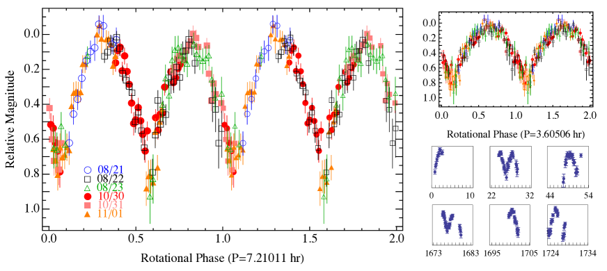
Figure 1.— Lightcurve of SQ₃₁₇. Large panel shows data phased with the best-fit spin period $P=7.21011$ hr. Two full rotations are shown. Smaller panels on the right show: (top) lightcurve phased with the possible but less likely period of $\sim$3.6 hr, and (bottom) measurements on each individual night with the $x$-axis (time) labeled in hours since MJD 55794.0 and the $y$-axis (unlabeled) equal to that of the figures above and to the left. The times are light-travel-time subtracted and so indicate when the light left SQ₃₁₇.

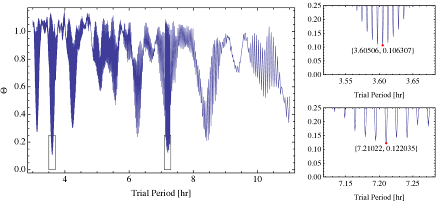
Figure 2.— Phase dispersion minimization periodogram for the SQ₃₁₇ data. Minima of the quantity $\Theta$ mark the most likely rotational periods. The two deepest minima are marked with boxes and enlarged on the right; the best-fit periods are shown in the insets together with the respective $\Theta$ value. Aliasing resulting from the way the data were sampled is visible in the insets.

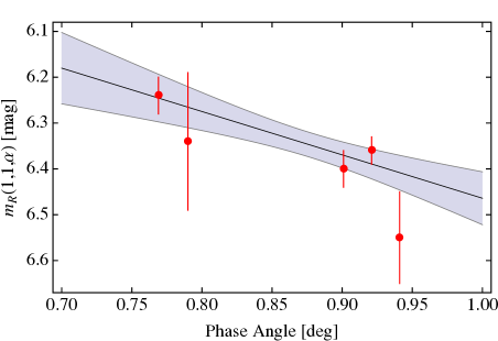
Figure 3.— Phase curve of SQ₃₁₇ as inferred from five measurements (filled circles with error bars). A least-squares fit to the data is indicated as a black line within a shaded, 1-$\sigma$ confidence region. The best fit has a slope $\beta=0.96\pm 0.41$ mag/$\arcdeg$ and intercept $m_{R}(1,1,0)=5.52\pm 0.36$ mag.

3.1. Rotational Lightcurve

Our photometry of SQ₃₁₇ resulted in $N=154$ measurements over 6 nights spanning a total interval of $T=1728$ hours (Figure 1), The brightness of SQ₃₁₇ varies visibly, by $\Delta m=0.85\pm 0.05$ mag peak-to-peak, taking only 1.8 hours to go from minimum to maximum brightness. The full extent of this variation is seen on multiple nights.

To search for periodicity in the data we employed two methods: the Phase Dispersion Minimization (PDM; Stellingwerf, 1978) and the String-Length Minimization (SLM; Dworetsky, 1983). PDM minimises the ratio, $\Theta$, between the scatter of the data phased with a trial period and that of the unphased data. The best-fit period will result in a lightcurve with the least scatter, hence minimising $\Theta$. SLM minimises the length of a segmented line connecting the data points phased with a trial period. Similarly to PDM, the best-fit period will result in a lightcurve with the smallest scatter around the real, periodic lightcurve and hence the shortest string length. Before running the period-search algorithms we corrected the observing times by subtracting the light-travel time from SQ₃₁₇ to Earth for each measurement.

Figure 2 shows the PDM periodogram for lightcurve periods ranging from 3 to 11 hours. Periods outside this range resulted in larger values of $\Theta$. Two strong PDM minima are apparent, one at $P_{1/2}\approx 3.6$ hr implying a single-peaked lightcurve with one maximum and one minimum per full rotation, and another at $P=2\times P_{1/2}\approx 7.2$ hr which folds the data onto a double-peaked lightcurve (Figure 1).

We favour the double-peaked solution, $P\approx 7.2$ hr, for three reasons. Firstly, a single-peaked lightcurve with a variation $\sim 0.85$ mag would have to be caused by a peculiar, large contrast, surface albedo pattern. The symmetry and regularity of the lightcurve suggest that the brightness variation is modulated instead by the elongated shape of SQ₃₁₇ as it rotates; lightcurves produced by shape are double peaked. Secondly, the double-peaked solution produces a lightcurve with slightly asymmetric minima, seen on more than one night. The single-peaked lightcurve minimum exhibits more scatter suggesting that it is a superposition of two different minima. Finally, the single-peaked period, $P_{1/2}\approx 3.6$ hr, would imply very fast rotation, at which SQ₃₁₇ would likely experience significant centripetal deformation for a plausible range of bulk densities and inner structures. The resulting elongated shape would produce a double-peaked lightcurve invalidating the premise that the lightcurve is single-peaked.

High resolution analysis near the $7.2$ hr lightcurve indicates a PDM minimum at $P_{\mathrm{PDM}}=7.21022$ hr, while using the SLM method, we obtained a best-fit period $P_{\mathrm{SLM}}=7.20999$ hr. We take as best-fit solution the mean of the two, $P=7.21011$ hr. To estimate the uncertainty in our period solution we employ (Horne & Baliunas, 1986)

$$\delta f=\frac{3\pi\,\sigma_{N}}{2\sqrt{N}\,T\,\Delta m}$$

where $\delta f$ is the uncertainty in the lightcurve frequency, $\sigma_{N}$ is the standard deviation of the lightcurve best-fit residuals (calculated using the model shown in Figure 7), $N=154$ is the number of data points, $T=1728$ hr is the total time spanned by the observations, and $\Delta m=0.85$ mag is the lightcurve variation. The frequency uncertainty is $\delta f=0.00002$ hr^-1 which corresponds to an uncertainty in the spin period $\delta P=0.00103$ hr. We therefore adopt as best period $P=7.210\pm 0.001$ hr.

3.2. Phase Curve

Owing to their large heliocentric distances, Kuiper belt objects are only observable from Earth at small phase angles, $\alpha<1.5\arcdeg$. Our observations span an approximate range $0.75<\alpha\,[\arcdeg]<0.95$ and we see a trend of fainter apparent magnitude with increasing phase angle. We fitted this observed phase darkening with a weighted linear model of the form

$$m_{R}(1,1,\alpha)=m_{R}(1,1,0)+\beta\,\alpha$$

where $m_{R}(1,1,0)$ is the absolute magnitude at zero phase angle and $\beta$ is the linear phase curve coefficient. The fit is plotted in Figure 3 where we show apparent magnitudes at lightcurve maxima. The best-fit zeropoint and slope are $m_{R}(1,1,0)=5.52\pm 0.36$ mag and $\beta=0.95\pm 0.41$ mag/$\arcdeg$. The phase function slope is steeper (although only by 2$\sigma$) than what is typically seen in other KBOs ($\beta_{\mathrm{KBO}}\sim 0.16$ mag/$\arcdeg$; Sheppard & Jewitt, 2002; Rabinowitz, Schaefer & Tourtellotte, 2007) and does not follow the trend for shallower phase functions observed in other objects associated with Haumea (Rabinowitz et al., 2008). We note that the phase function found above is consistent with the measurement $m_{R}=22.05\pm 0.02$ mag on 2008/08/30 (at phase angle $\alpha=0.62\arcdeg$, heliocentric distance $r=39.261$ AU and geocentric distance $\Delta=38.342$ AU) by Snodgrass et al. (2010). However, because of the narrow range of phase angles sampled, the uncertainty in the phase function slope is large so we are reluctant to draw strong implications from this result.

3.3. Shape Model

Table 4Model Fit Parameters

Model Type	$q$	$d$	$B/A$	$C/A$	$b/a$	$c/a$	$\rho$ [kg m-3]
Jacobi Ellipsoid	…	…	$0.55^{+0.05}_{-0.04}$	$0.41^{+0.02}_{-0.02}$	…	…	$861^{+33}_{-32}$
Roche Binary	$0.32^{+0.08}_{-0.07}$	$1.14^{+0.14}_{-0.04}$	$0.91^{+0.01}_{-0.03}$	$0.82^{+0.01}_{-0.02}$	$0.51^{+0.15}_{-0.07}$	$0.48^{+0.13}_{-0.07}$	$2671^{+88}_{-102}$

Note. — Columns are (1) Model used to fit lightcurve, (2) component mass ratio, (3) binary separation in units of $A+a$, (4) and (5) primary semimajor axes, (6) and (7) secondary semimajor axes, and (8) model bulk density.

The large photometric variability of SQ₃₁₇ suggests that the object has a highly elongated, possibly binary shape. Indeed, assuming that SQ₃₁₇ is close to hydrostatic equilibrium, its photometric range ($\Delta m=0.85$ mag) and spin frequency ($\omega=3.33$ day^-1) place it near the threshold between the Jacobi ellipsoid and the Roche binary sequences (Leone et al., 1984; Sheppard & Jewitt, 2004). To explore this issue further, we attempt to fit the lightcurve of SQ₃₁₇ using Jacobi ellipsoid and Roche binary hydrostatic equilibrium models. The choice of models of hydrostatic equilibrium is physically based and has the benefit of allowing the density of SQ₃₁₇ to be estimated.

We follow the procedure detailed in Lacerda & Jewitt (2007) which considers a grid of models spanning a range of Jacobi ellipsoid shapes, and Roche binary shapes, mass ratios and separations calculated using the formalism in Chandrasekhar (1963). Each model is rendered at multiple rotational phases to extract the lightcurve. Surface scattering is modelled as a linear combination of the Lambert and Lommel-Seeliger laws. The former mimics a perfectly diffuse surface and adequately describes a high-albedo, icy object displaying significant limb darkening. The latter is meant to simulate a low albedo, lunar-type surface with negligible limb darkening. These laws are linearly combined through a parameter, $k$, that varies between 0 (pure Lommel-Seeliger, lunar-type scattering) and 1 (pure Lambertian, icy-type scattering). The result is a collection of model lightcurves that can be compared to the one in Figure 1 to identify the best-fitting model.

As described in Lacerda & Jewitt (2007), the Jacobi ellipsoid model lightcurves are fully defined by the model’s triaxial shape (semi-axes $A,B,C$) in terms of the axis ratios $B/A$ and $C/A$, and by the coefficient $k$. The Roche binary lightcurves are entirely described by the binary component mass ratio $q$, the primary triaxial shape defined by the axes ratios $B/A$ and $C/A$, the secondary shape equally defined by the triaxial axis ratios $b/a$ and $c/a$, the binary separation, $d\geq 1$ (expressed in units of the sum of the primary and secondary semi-axes $A+a$), and the scattering parameter, $k$. Roche binaries are assumed to be tidally locked with the components aligned along their longest axes.

For simplicity and to keep the problem tractable we consider only models viewed equator-on. By allowing the observing geometry to vary as a free parameter we would increase the number of models that can match the lightcurve of SQ₃₁₇ and hence the overall degeneracy of the fitting procedure. Generally, off-equator geometries lead to slightly larger mass ratio solutions, but this has been shown not to have a significant effect on the inferred bulk density (Lacerda & Jewitt, 2007), arguably the most important derived property.

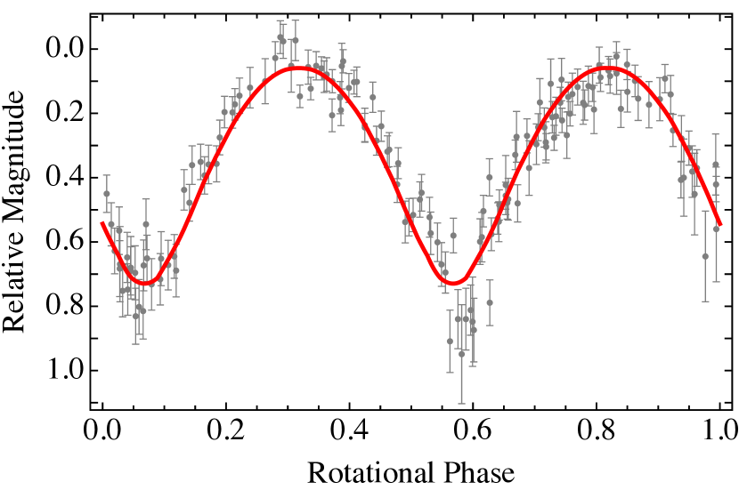
Figure 4.— Best-fit Jacobi ellipsoid lightcurve (solid line) plotted over the lightcurve data for SQ₃₁₇ (grey points). The corresponding Jacobi ellipsoid is shown in Figure 5.

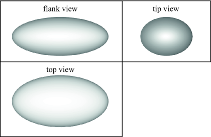
Figure 5.— Jacobi ellipsoid model that best fits the lightcurve of SQ₃₁₇.

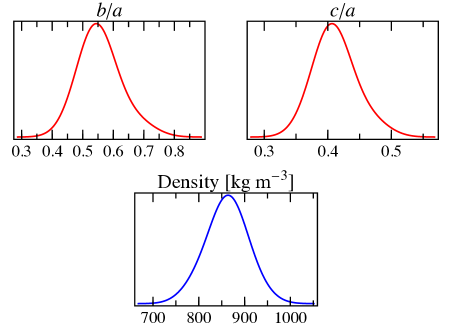
Figure 6.— Monte Carlo distribution of Jacobi ellipsoid parameters ($b/a$ and $c/a$) that fit the lightcurve of SQ₃₁₇. The Monte Carlo distribution of bulk density for these models is also shown.

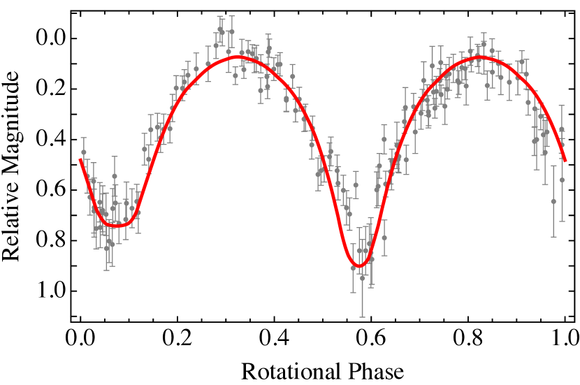
Figure 7.— Best-fit Roche binary lightcurve (solid line) plotted over the lightcurve data for SQ₃₁₇ (grey points). The corresponding Roche binary is shown in Figure 8.

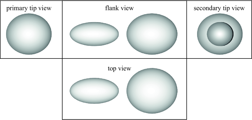
Figure 8.— Roche binary model that best fits the lightcurve of SQ₃₁₇.

8800

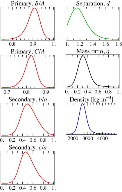
Figure 9.— Monte Carlo distribution of Roche binary parameters (mass ratio $q$, binary separation $d$, $B/A$, $C/A$, $b/a$ and $c/a$) that fit the lightcurve of SQ₃₁₇. The Monte Carlo distribution of bulk density for these models is also shown.

Each model lightcurve is adjusted (in phase and offset) to the data using a Levenberg-Marquardt algorithm and the best-fitting one is selected using a $\chi^{2}$ criterion. To explore the dependence of this procedure on the measurement uncertainties we employ a Monte Carlo approach: we generate $N=371$ bootstrapped instances of the lightcurve of SQ₃₁₇ by randomising each data point within its uncertainty error bar (errors are assumed normal with standard deviation equal to the size of the error bar). Finally, we find the best (minimum $\chi^{2}$) model for each bootstrapped version lightcurve and thus obtain the distribution of best-fit parameters.

Figure 4 shows the best-fitting Jacobi ellipsoid lightcurve and Figure 5 shows the corresponding model shape. The Monte Carlo distributions of best-fit parameters are shown in Figure 6. Figures 7, 8, and 9 show the best-fitting lightcurve, best model shape and parameter distributions for Roche binary models. Table 4 summarises the best-fit parameters for each model. The Roche binary fits are generally better with a typical $\chi^{2}\approx 1.62$ per degree of freedom compared to $\chi^{2}\approx 1.74$ per degree of freedom for the Jacobi ellipsoid models. The Roche binary model successfully fits the different minima in the lightcurve of SQ₃₁₇, unlike the Jacobi ellipsoid model. The mean scattering parameter for Jacobi ellipsoid fits is $k=0.1$, consistent with a low-albedo surface, while for Roche binaries we find a mean $k=0.4$, lending almost equal weights to (dark) lunar- and (bright) icy-type terrains. Higher $k$ values imply stronger limb darkening, which is needed to fit the different lightcurve minima.

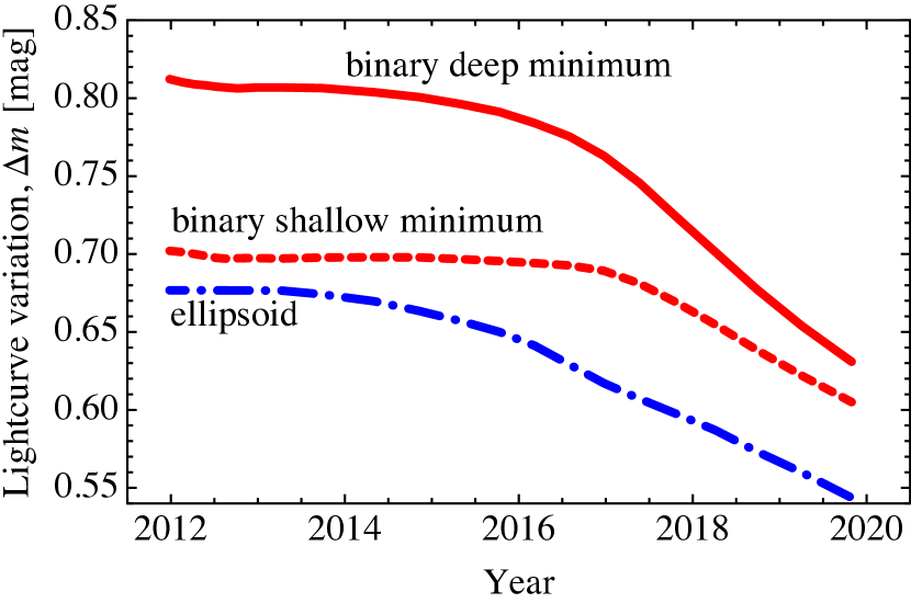
Figure 10.— Model lightcurve variation, $\Delta m$, as a function of time for the Jacobi ellipsoid (dash-dot, blue) and the Roche binary solution. In the case of the binary model, the changes for the shallow (dashed, red) and deep (solid, red) minima are shown. The change in $\Delta m$ plotted here is maximal as it assumes that the models have 90° obliquity.

3.4. Bulk Density

In §3.3 we found the Jacobi ellipsoid and Roche binary that best fit the lightcurve of SQ₃₁₇. Because these models assume hydrostatic equilibrium, their shapes are uniquely related to bulk density and spin period and allow us to use the latter to constrain the former. Each model shape is a function of the dimensionless parameter $\Omega^{2}=\omega^{2}/\left(\pi\,G\,\rho\right)$ where $\omega=2\pi/P$ is the angular rotation frequency ($P$ is the period), $G$ is the gravitational constant and $\rho$ is the bulk density. For a spin period $P=7.21$ hr, the density is then calculated as $\rho=280/\Omega^{2}$ kg m^-3.

Predictably, the two types of model imply very different bulk densities (Figures 6 and 9, Table 4). The Jacobi model fit yields $\Omega^{2}=0.325\pm 0.012$ and indicates a bulk density $\rho=860\pm 30$ kg m^-3, consistent with an icy composition. The Roche binary model has $\Omega^{2}=0.105\pm 0.004$ and leads to $\rho=2700\pm 100$ kg m^-3 suggesting a rock-rich bulk composition for SQ₃₁₇.

4. Discussion

As the analysis in §3.1 shows, SQ₃₁₇ oscillates in brightness by $\Delta m=0.85\pm 0.05$ mag, making it the second most variable KBO known, only surpassed by 2001 QG₂₉₈ (hereafter QG₂₉₈) with $\Delta m=1.14\pm 0.04$ mag (Sheppard & Jewitt, 2004). For bodies in hydrostatic equilibrium, lightcurve variation $\Delta m>0.9$ mag can only plausibly be explained by a tidally distorted, binary shape (Weidenschilling, 1980; Leone et al., 1984). That is the case of QG₂₉₈ which was sucessfully modelled as a Roche binary leading to an estimated bulk density near 660 kg m^-3 (Takahashi et al., 2004; Lacerda & Jewitt, 2007; Gnat & Sari, 2010). The Roche binary model received further support as QG₂₉₈ was re-observed in 2010 to show a predicted decrease in variability to $\Delta m=0.7$ magnitudes, which allowed the obliquity of the system to be estimated at very near 90$\arcdeg$ (Lacerda, 2011).

With $\Delta m=0.85$ mag and $P=7.21$ hr, SQ₃₁₇ lies at the threshold between the Jacobi and Roche sequences (Leone et al., 1984; Sheppard & Jewitt, 2004). Indeed, we find that SQ₃₁₇ can be fitted reasonably well both by Jacobi and Roche models. However, one important feature of the lightcurve, the asymmetric lightcurve minima, is only naturally fitted by the Roche binary model. The Jacobi model misses the data points that mark the faintest point of the lightcurve (Figure 4). In theory, a special arrangement of brighter and darker surface patches could be adopted to ensure that the Jacobi model fit the fainter lightcurve minimum. However, the binary model does not require any further assumptions and thus provides a simpler explanation for the asymmetric lightcurve minima. Figure 10 plots the change in lightcurve variation, $\Delta m$, for both models. To maximise the change, we assumed the models to have 90° obliquity so that an angular displacement, $\nu$, along the heliocentric orbit will translate into a change in aspect angle $\theta\approx\nu$ (Lacerda, 2011). The two models produce slightly different behaviour and future observations may help rule out one of the solutions.

The Jacobi and Roche model solutions predict significantly different bulk densities for SQ₃₁₇. The former is consistent with a density around 860 kg m^-3 which would indicate a predominantly icy interior and significant porosity. The Roche binary model implies a density close to 2670 kg m^-3, consistent with a rocky bulk composition. Densities higher than 2000 kg m^-3 have only been measured for the larger KBOs, Eris (Brown & Schaller, 2007; Sicardy et al., 2011), Pluto (Null, Owen & Synnott, 1993; Buie et al., 2006), Haumea (Rabinowitz et al., 2006; Lacerda & Jewitt, 2007) and Quaoar (Fornasier et al., 2013). Densities for objects with diameters similar to SQ₃₁₇ tend to fall in the range $500<\rho<1000$ kg m^-3 (Grundy et al., 2012; Stansberry et al., 2012) with the possible exception of (88611) Teharonhiawako with $\rho\approx 1400$ kg m^-3 (Osip, Kern & Elliot, 2003; Lellouch et al., 2013). If confirmed, the Roche model density of SQ₃₁₇ would make it one of the highest density known KBOs and the densest of its size.

In a scenario in which the Haumea family was produced by a collision that ejected the volatile-rich mantle of the proto-Haumea, its members would be expected to be mainly icy in composition, with high albedo surfaces. The Jacobi model density for SQ₃₁₇ would favour such a scenario (although the implied surface scattering is inconsistent with an icy, high albedo and high limb-darknening surface) whereas the Roche model density would be harder to explain in the context of the family. Haumea’s density $\rho\approx 2600$ kg m^-3 and water-ice spectrum implies a rocky core surrounded by a veneer of ice. If SQ₃₁₇ has high-density and was produced from a collision onto Haumea then it must be a fragment from the core material.

Broadband near-infrared photometry of SQ₃₁₇ suggests a surface rich in water ice (Snodgrass et al., 2010). Our measurements indicate a nearly solar surface colour $B-R=1.05\pm 0.18$ mag and a steep (although poorly constrained) phase function with slope $\beta=0.95\pm 0.41$ mag/$\arcdeg$. While the visible and infrared colours of SQ₃₁₇ match those of other members of the Haumea family, the phase function is much steeper.

The albedo of SQ₃₁₇ is unknown. Although its surface is blue and possibly water-ice rich, these properties do not necessary imply high albedo. For instance, 2002 MS₄ has blue colour ($B-R\approx 1.0$ mag; Peixinho et al., 2012) but low albedo ($p_{V}\approx 0.05$; Lellouch et al., 2013), and Quaoar displays strong water-ice absorption (Jewitt & Luu, 2004) despite its relatively dark ($p_{V}\approx 0.12$; Lellouch et al., 2013) and red surface ($B-R\approx 1.6$ mag; Peixinho et al., 2012). Water ice has been spectroscopically detected on objects with albedos as low as 0.04, e.g. Chariklo (Guilbert et al., 2009), and as high as 0.80, e.g. Haumea (Trujillo et al., 2007).

The shape models and density estimates presented above assume an idealised fluid object in hydrostatic equilibrium. As a limiting case, the simplification is useful because it offers a simple and unique relation between shape, spin period and bulk density. However, SQ₃₁₇ is a solid body and likely behaves differently. Holsapple (2001, 2004) have studied extensively the equilibrium configurations of rotating solid bodies—sometimes termed “rubble piles”—that possess no tensile strength but that can retain shapes bracketing the hydrostatic solution due to pressure-induced, internal friction. Similar studies were performed for Roche figures of equilibrium by Sharma (2009). The deviation from the hydrostatic equilibrium solution is usually quantified in terms of an increasing angle of friction, $0\mathrm{\arcdeg}<\phi<90\mathrm{\arcdeg}$. For a positive value of $\phi$, a range of bulk densities (which includes the hydrostatic equilibrium solution) is possible for an object with a given shape and spin rate.

For a plausible range of albedos, SQ₃₁₇ has an equivalent diameter in the range $150<D<450$ km. The giant planet icy moons in the same size range (Amalthea at Jupiter and Mimas, Phoebe and Janus at Saturn; Hyperion has chaotic rotation and is ignored) lie at the threshold between near hydrostatic shapes and slightly more irregular configurations (Thomas, 2010; Castillo-Rogez et al., 2012). When approximated by triaxial ellipsoids and plotted on the diagrams of Holsapple (2001), the shapes, spins and densities of these moons are consistent with angles of friction $\phi<5\arcdeg$ (see also Sharma, 2009). Similar values of $\phi$ are found for most large, approximately triaxial asteroids (Sharma, Jenkins & Burns, 2009). If we take our Jacobi ellipsoid solution for SQ₃₁₇ and assume an angle of friction $\phi=5\arcdeg$ then we find that its density should lie in the range $670<\rho<1100$ kg m^-3, i.e. a 30% departure from the idealised hydrostatic equilibrium solution. A similar uncertainty applied to the Roche binary density estimate yields a range $2050<\rho<3470$ kg m^-3.

5. Summary

We present time-resolved photometric observations of Kuiper belt object 2003 SQ₃₁₇ obtained in August and October 2011 to investigate its nature. Our results can be summarised as follows:

1. SQ₃₁₇ exhibited a highly variable photometric lightcurve with a peak-to-peak range $\Delta m=0.85\pm 0.05$ magnitudes and period $P=7.210\pm 0.001$ hours. The object has an almost solar broadband colour $B-R=1.05\pm 0.18$ mag, making it one of the bluest KBOs known. The phase function of SQ₃₁₇ is well matched by a linear relation with intercept $m_{R}(1,1,0)=5.52\pm 0.36$ mag and slope $\beta=0.96\pm 0.41$ mag/$\arcdeg$. This linear phase function is consistent with an earlier measurement obtained in 2008 at phase angle $\alpha=0.62\arcdeg$.

2. The lightcurve implies that SQ₃₁₇ is highly elongated in shape. Assuming that the object is in hydrostatic equilibrium, we find that the lightcurve of SQ₃₁₇ is best fit by a compact Roche binary model with mass ratio $q\sim 0.3$, and triaxial primary and secondary components with axes ratios $B/A\sim 0.9$, $C/A\sim 0.8$ and $b/a\sim c/a\sim 0.5$, separated by $d\sim 1.1(A+a)$. The data are also adequately fitted by a highly elongated, Jacobi triaxial ellipsoid model with axes ratios $B/A\sim 0.55$ and $C/A\sim 0.41$. Observations in this decade may be able to rule out one of the two solutions.

3. If SQ₃₁₇ is a Roche binary then its bulk density is approximately 2670 kg ^-3. This model-dependent density implies rock-rich composition for this object. However, if SQ₃₁₇ is a Jacobi ellipsoid we find a significantly lower density, $\rho\approx 860$ kg m^-3 consistent with an icy, porous interior. These density estimates become uncertain at the 30% level if we relax the hydrostatic assumption and account for “rubble pile”-type configurations.

References

- Barkume, Brown & Schaller (2006) Barkume K. M., Brown M. E., Schaller E. L., 2006, ApJ, 640, L87
- Brown et al. (2007) Brown M. E., Barkume K. M., Ragozzine D., Schaller E. L., 2007, Nature, 446, 294
- Brown et al. (2005) Brown M. E. et al., 2005, ApJ, 632, L45
- Brown & Schaller (2007) Brown M. E., Schaller E. L., 2007, Science, 316, 1585
- Buie et al. (2006) Buie M. W., Grundy W. M., Young E. F., Young L. A., Stern S. A., 2006, AJ, 132, 290
- Buzzoni et al. (1984) Buzzoni B. et al., 1984, The Messenger, 38, 9
- Carry et al. (2012) Carry B., Snodgrass C., Lacerda P., Hainaut O., Dumas C., 2012, A&A, 544, A137
- Castillo-Rogez et al. (2012) Castillo-Rogez J. C., Johnson T. V., Thomas P. C., Choukroun M., Matson D. L., Lunine J. I., 2012, Icarus, 219, 86
- Chandrasekhar (1963) Chandrasekhar S., 1963, ApJ, 138, 1182
- Dumas et al. (2011) Dumas C., Carry B., Hestroffer D., Merlin F., 2011, A&A, 528, A105
- Dworetsky (1983) Dworetsky M. M., 1983, MNRAS, 203, 917
- Fornasier et al. (2013) Fornasier S. et al., 2013, A&A, 555, A15
- Gnat & Sari (2010) Gnat O., Sari R., 2010, ApJ, 719, 1602
- Grundy et al. (2012) Grundy W. M. et al., 2012, Icarus, 220, 74
- Guilbert et al. (2009) Guilbert A. et al., 2009, A&A, 501, 777
- Hartmann & Cruikshank (1978) Hartmann W. K., Cruikshank D. P., 1978, Icarus, 36, 353
- Holmberg, Flynn & Portinari (2006) Holmberg J., Flynn C., Portinari L., 2006, MNRAS, 367, 449
- Holsapple (2001) Holsapple K. A., 2001, Icarus, 154, 432
- Holsapple (2004) Holsapple K. A., 2004, Icarus, 172, 272
- Horne & Baliunas (1986) Horne J. H., Baliunas S. L., 1986, ApJ, 302, 757
- Jewitt & Luu (2004) Jewitt D. C., Luu J., 2004, Nature, 432, 731
- Lacerda (2009) Lacerda P., 2009, AJ, 137, 3404
- Lacerda (2011) Lacerda P., 2011, AJ, 142, 90
- Lacerda, Jewitt & Peixinho (2008) Lacerda P., Jewitt D., Peixinho N., 2008, AJ, 135, 1749
- Lacerda & Jewitt (2007) Lacerda P., Jewitt D. C., 2007, AJ, 133, 1393
- Landolt (1992) Landolt A. U., 1992, AJ, 104, 340
- Leinhardt, Marcus & Stewart (2010) Leinhardt Z. M., Marcus R. A., Stewart S. T., 2010, ApJ, 714, 1789
- Lellouch et al. (2010) Lellouch E. et al., 2010, A&A, 518, L147
- Lellouch et al. (2013) Lellouch E. et al., 2013, A&A (in press)
- Leone et al. (1984) Leone G., Paolicchi P., Farinella P., Zappala V., 1984, A&A, 140, 265
- Null, Owen & Synnott (1993) Null G. W., Owen W. M., Synnott S. P., 1993, AJ, 105, 2319
- Osip, Kern & Elliot (2003) Osip D. J., Kern S. D., Elliot J. L., 2003, Earth Moon and Planets, 92, 409
- Peixinho et al. (2012) Peixinho N., Delsanti A., Guilbert-Lepoutre A., Gafeira R., Lacerda P., 2012, A&A, 546, A86
- Rabinowitz et al. (2006) Rabinowitz D. L., Barkume K., Brown M. E., Roe H., Schwartz M., Tourtellotte S., Trujillo C., 2006, ApJ, 639, 1238
- Rabinowitz et al. (2008) Rabinowitz D. L., Schaefer B. E., Schaefer M., Tourtellotte S. W., 2008, AJ, 136, 1502
- Rabinowitz, Schaefer & Tourtellotte (2007) Rabinowitz D. L., Schaefer B. E., Tourtellotte S. W., 2007, AJ, 133, 26
- Ragozzine & Brown (2007) Ragozzine D., Brown M. E., 2007, AJ, 134, 2160
- Schaller & Brown (2008) Schaller E. L., Brown M. E., 2008, ApJ, 684, L107
- Schlichting & Sari (2009) Schlichting H. E., Sari R., 2009, ApJ, 700, 1242
- Sharma (2009) Sharma I., 2009, Icarus, 200, 636
- Sharma, Jenkins & Burns (2009) Sharma I., Jenkins J. T., Burns J. A., 2009, Icarus, 200, 304
- Sheppard & Jewitt (2004) Sheppard S. S., Jewitt D., 2004, AJ, 127, 3023
- Sheppard & Jewitt (2002) Sheppard S. S., Jewitt D. C., 2002, AJ, 124, 1757
- Sicardy et al. (2011) Sicardy B. et al., 2011, Nature, 478, 493
- Snodgrass & Carry (2013) Snodgrass C., Carry B., 2013, The Messenger, 152, 14
- Snodgrass et al. (2010) Snodgrass C., Carry B., Dumas C., Hainaut O., 2010, A&A, 511, A72
- Snodgrass et al. (2008) Snodgrass C., Saviane I., Monaco L., Sinclaire P., 2008, The Messenger, 132, 18
- Stansberry et al. (2012) Stansberry J. A. et al., 2012, Icarus, 219, 676
- Stellingwerf (1978) Stellingwerf R. F., 1978, ApJ, 224, 953
- Takahashi et al. (2004) Takahashi S., Shinokawa K., Yoshida F., Mukai T., Ip W. H., Kawabata K., 2004, Earth, Planets, and Space, 56, 997
- Thomas (2010) Thomas P. C., 2010, Icarus, 208, 395
- Trujillo et al. (2007) Trujillo C. A., Brown M. E., Barkume K. M., Schaller E. L., Rabinowitz D. L., 2007, ApJ, 655, 1172
- Volk & Malhotra (2012) Volk K., Malhotra R., 2012, Icarus, 221, 106
- Weidenschilling (1980) Weidenschilling S. J., 1980, Icarus, 44, 807