Algorithms for group isomorphism via
group extensions and cohomology

Abstract

The isomorphism problem for finite groups of order $n$ (GpI) has long been known to be solvable in $n^{\log n+O(1)}$ time, but only recently were polynomial-time algorithms designed for several interesting group classes. Inspired by recent progress, we revisit the strategy for GpI via the extension theory of groups.

The extension theory describes how a normal subgroup $N$ is related to $G/N$ via $G$, and this naturally leads to a divide-and-conquer strategy that “splits” GpI into two subproblems: one regarding group actions on other groups, and one regarding group cohomology. When the normal subgroup $N$ is abelian, this strategy is well-known. Our first contribution is to extend this strategy to handle the case when $N$ is not necessarily abelian. This allows us to provide a unified explanation of all recent polynomial-time algorithms for special group classes.

Guided by this strategy, to make further progress on GpI, we consider central-radical groups, proposed in Babai et al. (SODA 2011): the class of groups such that $G$ mod its center has no abelian normal subgroups. This class is a natural extension of the group class considered by Babai et al. (ICALP 2012), namely those groups with no abelian normal subgroups. Following the above strategy, we solve GpI in $n^{O(\log\log n)}$ time for central-radical groups, and in polynomial time for several prominent subclasses of central-radical groups. We also solve GpI in $n^{O(\log\log n)}$ time for groups whose solvable normal subgroups are elementary abelian but not necessarily central. As far as we are aware, this is the first time there have been worst-case guarantees on a $n^{o(\log n)}$-time algorithm that tackles both aspects of GpI—actions and cohomology—simultaneously.

Prior to this work, the best proven upper bounds on algorithms for groups with central radicals were $n^{O(\log n)}$, even for groups with a central radical of constant size, such as $\operatorname{Rad}(G)=Z(G)=\mathbb{Z}_{2}$. To develop our new algorithms we utilize several mathematical results on the detailed structure of cohomology classes, as well as algorithmic results for code equivalence, coset intersection and cyclicity testing of modules over finite-dimensional associative algebras. We also suggest several promising directions for future work.

1 Introduction

The group isomorphism problem (GpI) is to determine whether two finite groups are isomorphic. For groups of order $n$, the easy $n^{\log n+O(1)}$-time algorithm [FN70, Mil78] for the general case of GpI has barely seen any asymptotic improvement over the past four decades; it was improved recently to $n^{1/4\log n+O(1)}$ by Rosenbaum [Ros13a] (see [GR16, Sec. 2.2]), but even the extensive body of work on practical algorithms led by Eick, Holt, Leedham-Green and O’Brien (e. g., [BEO02, ELGO02, BE99, CH03])—resulting in most of the functional algorithms in use today—was recently found [Wil14] to only improve the constant in the exponent, still resulting in a $n^{\Theta(\log n)}$-time algorithm for the general case. The past few years have witnessed a resurgence of activity on worst-case guaranteed algorithms for this problem [LG09, BCGQ11, QST11, Wag11, LW12, BQ12, BCQ12, Ros13b, Ros13a, BMW15, GQ15].

Before introducing these works and our results, we recall why group isomorphism is an intriguing problem from the complexity-theoretic perspective, even when the groups are given by their multiplication tables. (See Remark 1.1 below.) We call this version of the problem CayleyGpI. As CayleyGpI reduces to Graph Isomorphism (GraphI) (see, e. g., the book [KST93]), CayleyGpI currently has an intermediate status: It is not $\mathsf{NP}$-complete unless $\mathsf{PH}$ collapses [BHZ87, BM88], and is not known to be in $\mathsf{P}$. In addition to its intrinsic interest, resolving the exact complexity of GpI is a tantalizing question. Further, there is a surprising connection between CayleyGpI and the Geometric Complexity Theory program (see, e. g., [Mul11] and references therein): Techniques from CayleyGpI were used to solve cases of Lie Algebra Isomorphism that have applications in Geometric Complexity Theory [Gro12].

In a survey article [Bab95] in 1995, after enumerating several isomorphism-type problems including GraphI and GpI, Babai expressed the belief that CayleyGpI might be the only one expected to be in $\mathsf{P}$. Indeed, in many ways CayleyGpI seems easier than GraphI: There is a simple $n^{\log n+O(1)}$-time algorithm for GpI, whereas the best known algorithm for GraphI takes time $2^{(\log n)^{c}}$ for some $c\geq 3$ [Bab16] and is quite complicated. There is a polynomial-time reduction from CayleyGpI to GraphI, yet there is provably no $\mathsf{AC}^{0}$ reduction in the opposite direction [CTW10]. The reduction $\mbox{\sc CayleyGpI}\leq\mbox{\sc GraphI}$ means that CayleyGpI stands as an obstacle to putting GraphI into $\mathsf{P}$; in light of the recent quasi-polynomial-time algorithm for GraphI [Bab16], this obstacle has become much more salient (the previous best algorithm for GraphI was so far from quasi-polynomial that there were clearly obstacles to be overcome before CayleyGpI became a serious obstacle, but many of those obstacles have now been overcome). Further, GraphI is as hard as its counting version, whereas no such counting-to-decision reduction is known for GpI. Finally, whereas the smallest standard complexity class known to contain GraphI is $\mathsf{NP}\cap\mathsf{coAM}$, Arvind and Torán [AT11] showed that CayleyGpI for solvable groups is in $\mathsf{NP}\cap\mathsf{coNP}$ under a plausible assumption, weaker than that needed to show $\mbox{\sc GraphI}\in\mathsf{coNP}$ (recall that a group is solvable if all its composition factors are abelian, or equivalently if the derived series $G_{0}=G$, $G_{i+1}=[G_{i},G_{i}]$ terminates in the identity).

Despite this situation and considerable attention to GpI, prior to 2009 the actual developments towards algorithms with worst-case guaranteed running time polynomial in $|G|$ essentially stopped at abelian groups, although there have been impressive practical advances (see, e. g., the theses [Smi94, How12] and references therein for nice overviews). Isomorphism of abelian groups has long been known to be solvable in polynomial time [Sav80, Ili85, Vik96, Kav07]. The next natural group class after abelian groups—class 2 nilpotent groups, whose quotient by their center is abelian—turns out to be formidable (see [GZ91, LW12, BMW15] for efficient algorithms in some restricted cases).

Beginning in 2009 there were several advances on worst-case guaranteed algorithms, starting with Le Gall [LG09]. In [BCQ12], following [BCGQ11], Babai et al. developed a polynomial-time algorithm for groups with no abelian normal subgroups. This suggests the presence of abelian normal subgroups as a bottleneck. With this in mind, Babai and Qiao [BQ12] developed a polynomial-time algorithm for a special class of non-nilpotent solvable groups, building on [LG09, QST11]; this was recently extended by the present authors to the so-called groups of tame extensions [GQ15]. In [LW12], Lewis and Wilson made intriguing progress on $p$-groups: They gave a polynomial-time algorithm for quotients of generalized Heisenberg groups, a decently large subclass of $p$-groups of class 2. Rosenbaum’s recent works [Ros13b, Ros13a] (some of them building on ideas of Wagner [Wag11]) lead to an $n^{1/4\log n+O(1)}$-time algorithm for GpI (see [GR16, Sec. 2.2]). To summarize, at present it is crucial to understand indecomposable groups with abelian normal subgroups to develop $n^{o(\log n)}$-time algorithms.

Given these developments, we are at an interesting crossroads: First, as several nontrivial algorithms with worst-case guarantees have recently been developed (or worst-case guarantees proven for previously known algorithms), it is reasonable to reflect back to see if there is some common pattern or structure to these results. Second, of course, we should continue to improve the state of the art by developing more $n^{o(\log n)}$-time algorithms for special group classes. Finally, class 2 nilpotent groups seem to remain the bottleneck, but despite heuristic evidence, it is still desirable to formalize a reduction from the general case to this seeming bottleneck.

In this paper we contribute to all three of the preceding aspects. Our contributions are twofold: (1) we show how a general strategy for group isomorphism from the mathematics literature can be used to bound the worst-case complexity; and (2) using that strategy, we develop an $n^{O(\log\log n)}$-time algorithm for a group class proposed in [BCGQ11], and polynomial-time algorithms for some prominent subclasses thereof. The worst-case analysis of this strategy also helps to explain in a unified way the recent successes on other group classes [LG09, QST11, BQ12, BCGQ11, BCQ12, LW12, GQ15], which can be viewed as adding class-specific tactics to the general strategy. We also explain how these results may help to reduce general GpI to the class 2 nilpotent case.

Remark 1.1 (On efficient implementation versus computational complexity).

There are naturally two audiences for this paper, who might view it quite differently: (A) computational complexity theorists / algorithms theory researchers, and (B) computational group theorists. To some in the latter group, much of the content of this paper is surely well-known, and to them perhaps not even worth writing down at this point in history. To them, we would like to highlight our results on nonabelian cohomology (Section 3) and the use of Guralnick–Kantor–Kassabov–Lubotzky [GKKL07], which we believe may be new even in light of the large body of work in that community. We would also like to point out that the remainder of the paper will likely seem new to computational complexity theorists, despite seeming trivial to computational group theorists. As so often happens when ideas from one area B (in this case, classical and computational group theory) are imported to another area A (computational complexity), area B may view the results as trivial while area A may view them as a nontrivial advance. However, while much of this paper is targeted at computational complexity theorists and so has this flavor, we believe that some of the results (as mentioned above) will be new to both communities.

As discussed above, there are good reasons (e. g., related to GraphI) to be interested in the getting the asymptotic complexity of GpI down to polynomial in the order of the group, independently of its (ir)relevance to practical implementation. Combined with the fact that all of the practical algorithms put together still leave the worst-case bound at $|G|^{\Theta(\log|G|)}$ [Wil14], we thus state our runtime bounds as a function of $n=|G|$. Nonetheless, our algorithms are fairly agnostic to the method of input, and in particular do not depend on the input being a Cayley table. That is, when the runtime of an algorithm is at least quadratic in the order of the group, even if the group is input as a black box, the algorithm may first enumerate the entire multiplication table, and then proceed from there.

Except in a few cases, we do not bother to estimate multiplicative constants, nor even constant exponents, in most of our algorithms. The current inability to get a general algorithm with run-time $|G|^{o(\log|G|)}$ [Wil14] suggests that this is a potentially deep research topic, and getting algorithms with guaranteed run-time $|G|^{O(1)}$ can be seen as a first step in understanding the difficulties involved (not to mention its complexity-theoretic interest). Furthermore, there is non-trivial precedent for synergistic interaction between worst-case analyses and practical algorithms, as reflected in, e. g., A. Seress’s pioneering implementations in GAP [GG13] of theoretically-proven fast algorithms for permutation groups (see, e. g., [Ser03]). Therefore, although we do not deal with issues of practical algorithms in this paper, it is our sincere hope that this great tradition will continue in future work.

1.1 Main results

The classes of groups we consider are natural extensions of the class of groups considered in [BCGQ11, BCQ12], and are additionally motivated by the Babai–Beals filtration [BB99] (resurrecting certain ideas that go back to Fitting [Fit33]), and the Cannon–Holt approach to group isomorphism in the practical setting [CH03]. We go into the details of the Babai–Beals filtration and the Cannon–Holt approach in Section 8. Here we merely give enough of a flavor to help motivate the classes of groups we consider.

Important in both the Babai–Beals filtration and the Cannon–Holt approach is the solvable radical. The solvable radical $\operatorname{Rad}(G)$ of a group $G$ is the unique maximum solvable normal subgroup of $G$. Note that the center $Z(G)$, as an abelian normal subgroup, is contained in $\operatorname{Rad}(G)$. $G/\operatorname{Rad}(G)$ contains no solvable normal subgroups, side-stepping the currently intractable obstacle of solvable groups. Babai et al. [BCQ12] give a polynomial-time algorithm for isomorphism of groups with no solvable normal subgroups (equivalently, no abelian normal subgroups); following them, we call such groups “semisimple.”

We mainly consider the class of groups whose solvable radical coincides with its center, that is, $\operatorname{Rad}(G)=Z(G)$; in Section 6.2 we also consider groups whose solvable radical is abelian, but need not be contained in the center. The former class, which we refer to as groups with central radicals or central-radical groups for short, is a natural extension of the class of semisimple groups and a natural stepping stone towards general groups (see Figure 1 below). Note that for such groups the solvable radical is necessarily abelian. Besides the motivations mentioned above, central-radical groups also cover a class of groups that is well-studied in finite group theory (see Appendix B). In the theory of Lie groups, central-radical groups correspond to the well-studied and important class of reductive Lie groups, which are important throughout mathematics and physics, often because of their nice representation-theoretic properties.

We use the strategy outlined in Section 1.3 below to achieve the following results. For groups with central radicals, we give an $n^{O(\log\log n)}$-time algorithm in general, and for several subclasses of groups with central radicals we give polynomial-time algorithms. We also give similarly efficient algorithms for groups with elementary abelian, but not necessarily central, radicals. Prior to this work, the best proven upper bounds on algorithms for groups with central radicals were $n^{O(\log n)}$, even for groups with a central radical of constant size, such as $\operatorname{Rad}(G)=Z(G)=\mathbb{Z}_{2}$.

Recall that for any groups $G$ and $H$, the set of isomorphisms between them is either empty or a coset of the automorphism group $\mathrm{Aut}(G)$ in the group of permutations of the disjoint union $G\sqcup H$. We say that the coset of isomorphisms can be found if one isomorphism $G\stackrel{{\scriptstyle\cong}}{{\to}}H$ and a generating set for $\mathrm{Aut}(G)$ can be found. Finding the full coset of isomorphisms—rather than just deciding GpI or finding a single isomorphism—is often useful in recursively building algorithms for larger group classes from those for smaller classes.

Theorem A (=Corollary 6.2).

Isomorphism of central-radical groups of order $n$ can be decided in time $n^{c\log\log n+O(1)}$, for $c=1/\log_{2}(60)\approx 0.169$. Furthermore, if the radical is elementary abelian, the coset of isomorphisms can be found in the same time bound.

The algorithm in the above theorem in fact runs in polynomial time when the order or structure of the semisimple quotient $G/\operatorname{Rad}(G)$ is bounded as follows. Recall that a normal subgroup of $G$ is minimal if it is nontrivial and does not contain any smaller normal subgroups of $G$. The number of minimal normal subgroups of $G/\operatorname{Rad}(G)$ is always at most $\log_{60}n$; if it happens to be just slightly smaller, then we have:

Corollary 6.3.

Let $G$ and $H$ be central-radical groups of order $n$. If $G/\operatorname{Rad}(G)$ has $O(\frac{\log n}{\log\log n})$ minimal normal subgroups, isomorphism between $G$ and $H$ can be decided in $\mathrm{poly}(n)$ time. Furthermore, if the radical is elementary abelian, the coset of isomorphisms can be found in the same time bound.

In particular, this includes groups $G$ satisfying $|G/\operatorname{Rad}(G)|\leq n^{O(1/\log\log n)}$, but also many groups where $G/\operatorname{Rad}(G)$ is much larger. Both of these theorems are in fact corollaries of our more general Theorem 6.1 together with previous results on semisimple groups [BCGQ11], but we defer the statement of Theorem 6.1 until Section 6, as the above results make its significance clearer.

For groups with elementary abelian radicals—even if they are not central—we get the same conclusions. This requires us to simultaneously solve Action Compatibility and Cohomology Class Isomorphism. We combine the above techniques with a novel reduction to known representation-theoretic algorithms [CIK97] to get:

Theorem B (=Corollaries 6.12 and 6.13).

Isomorphism of groups of order $n$ with elementary abelian radicals can be decided, and the coset of isomorphisms found, in time $n^{c\log\log n+O(1)}$, for $c=1/\log_{2}(60)\approx 0.169$.

If furthermore $G/\operatorname{Rad}(G)$ has $O(\frac{\log n}{\log\log n})$ normal subgroups, isomorphism can be decided, and the coset of isomorphisms found, in $\mathrm{poly}(n)$ time.

We then consider central-radical groups with $G/\operatorname{Rad}(G)$ a direct product of nonabelian simple groups. Although this may seem restrictive, this class of groups is quite natural. In group theory, this class is closely related to the generalized Fitting subgroups (see, e. g., [Suz86, Ch. 6, §6] and [Asc00, Ch. 11], as well as Appendix B). Also, within central-radical groups, this class has two characterizations: (1) the last two of the four levels of the Babai–Beals filtration are trivial (see Section 8.2); or (2) those groups that are equal to their generalized Fitting subgroup (see Appendix B). Our next result gives polynomial-time algorithms for this group class, which includes, for example, central extensions of $\mathbb{Z}_{p}^{\Theta(\log n)}$ by $A_{k}^{\Theta(\log n)}$, which do not satisfy the conditions of the results above.

Theorem C (=7.1).

Isomorphism between two groups $G_{1},G_{2}$ with central, elementary abelian radicals can be decided, and the coset of isomorphisms found, in $\mathrm{poly}(|G_{i}|)$ time if either:

1. $G_{1}/\operatorname{Rad}(G_{1})$ is a direct product of simple groups; or

2. $G_{1}/\operatorname{Rad}(G_{1})$ is a direct product of perfect groups, each of order $O(1)$.

More importantly, we believe the techniques that go into proving this theorem are worth noting: we rely on a detailed analysis of the structure of the cohomology classes specific to this group class (see Section 7.1, and the use of the powerful results of [GKKL07]) to allow for the application of known algorithmic techniques, including singly-exponential-time algorithms for Linear Code Equivalence [Bab10] (see [BCGQ11, Thm. 7.1]) and Coset Intersection [Bab83, Luk99] (see also [Bab08, BKL83]).

1.2 Motivation for the classes of groups considered

Aside from the motivations already mentioned above, Figure 1 gives the general idea of where this paper fits in the picture of a larger approach towards putting GpI into $\mathsf{P}$. The figure is neither complete nor 100% accurate in terms of the landscape of groups and algorithms for GpI, but is more or less correct for algorithms with worst-case guarantees at a large scale.

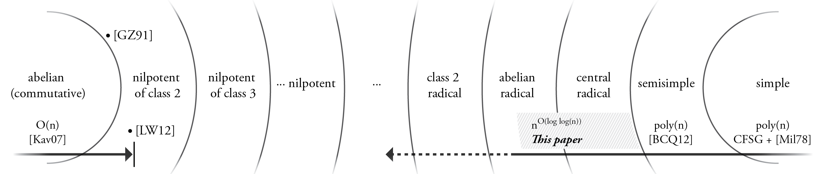
Figure 1: Some progress on group isomorphism. The arrow on the left indicates that the techniques for abelian groups hit a wall before class 2 nilpotent groups. The arrow on the right indicates the recent progress at the “opposite end of the spectrum,” including this paper and prospects for future progress.

While central-radical groups may seem to be only a slight extension of semisimple groups, they in fact differ significantly from previous classes of groups with $n^{o(\log n)}$-time isomorphism algorithms. In particular, most previous $n^{o(\log n)}$-time algorithms for GpI of special group classes only consider one of the two main aspects of GpI, namely actions (in Section 4.2, we briefly indicate how actions are used in [LG09, QST11, BQ12, BCGQ11, BCQ12]). On the other hand, to work with groups with central radicals, we need to focus on the other main aspect of the problem, namely cohomology (see Section 1.3).

Our results also suggest one more step towards a formal reduction from the general case to nilpotent groups of class 2. In particular, in Proposition 3.13 and Remark 3.14, we show that for groups $G$ where the action of $G$ on $\operatorname{Rad}(G)$ by conjugation is essentially trivial (technically: the action is by inner automorphisms of $\operatorname{Rad}(G)$) and $\mathrm{Aut}(Z(\operatorname{Rad}(G)))$ is small, GpI reduces to isomorphism of central-radical groups and isomorphism of solvable groups, separately. Thus, if isomorphism of central-radical groups could be decided in polynomial time, then GpI for this class of groups would reduce to GpI for solvable groups. Note that central-radical groups arise here naturally, by considering cases in which the relationship between $G/\operatorname{Rad}(G)$ and $\operatorname{Rad}(G)$ is simple. This is just one example of how we believe our ideas point towards a possible reduction from the general case to nilpotent groups; some other ideas in this paper may also be useful in this regard (see Section 8.3).

1.3 A strategy via group extensions and cohomology

In this paper we use the theory of group extensions (which we describe briefly in this section, and in more detail in Section 2, and give expository preliminaries in Appendix A; for textbook treatments, see, e. g., [Rob96, Chapter 11] and [Rot94, Chapter 7]) to show that the group isomorphism problem “splits” into two subproblems—one coming from actions of groups on other groups (Action Compatibility), and the other coming from group extensions and cohomology (Cohomology Class Isomorphism), which we explain below. We note that Besche and Eick have proposed this splitting in a slightly different setting, under the name “strong isomorphism” [BE99]. In the abstract theory of finite groups this splitting is standard material; the contribution here is the observation that this standard material can be used to prove worst-case algorithmic guarantees and that doing so is useful and even formally necessary to resolve the complexity of GpI. We also extend this approach to the setting where the normal subgroup can be non-abelian. For the converse direction, we observe that special cases of these subproblems reduce to GpI under polynomial-time reductions (Section 4.3). We summarize these results in:

Facts 4.1, 4.3, and Lemmas 2.3, 3.7 (“Splitting” GpI into actions and cohomology).

• For coprime extensions Action Compatibility $\equiv_{m}^{p}\mbox{\sc GpI}$.

• For $p$-groups of class 2, when $p>2$, Cohomology Class Isomorphism $\equiv_{m}^{p}\mbox{\sc GpI}$.

• GpI for groups with a normal subgroup from one class of groups $\mathcal{N}$ and a quotient from a class of groups $\mathcal{Q}$ reduces to solving GpI in $\mathcal{N}$, solving it in $\mathcal{Q}$, and simultaneously solving Action Compatibility and Cohomology Class Isomorphism.

A “simultaneous solution” to these two problems is possible because they have the same space of potential solutions, namely certain automorphisms of certain groups; a simultaneous solution is an automorphism that is simultaneously a solution for both problems. See Section 1.4 and Lemma 2.3 for more details.

Most previous complexity-theoretic results on GpI have focused on some combination of algorithmic techniques and Action Compatibility. In this paper, for the first time from the worst-case complexity perspective, we make progress on Cohomology Class Isomorphism.

We now explain this “splitting” and the problems mentioned above informally. Consider the following natural strategy for testing whether $G$ is isomorphic to $H$. If $G$ is simple, then isomorphism can be tested in polynomial time as $G$ is generated by at most two elements (Fact 5.1). If $G$ is not simple, then it has some normal subgroup $N\unlhd G$, and we may try to use a divide-and-conquer strategy by first solving the isomorphism problem for $N$ and $G/N$. However, even if we find $M\unlhd H$ such that $N\cong M$ and $G/N\cong H/M$, this is typically not sufficient to conclude that $G\cong H$: e. g., $\mathbb{Z}_{4}$ and $\mathbb{Z}_{2}\times\mathbb{Z}_{2}$ both have $\mathbb{Z}_{2}$ as a normal subgroup, with corresponding quotient $\mathbb{Z}_{2}$. We must then understand how the groups $N$ and $G/N$ “glue” back together to get $G$. $G$ is called an extension of $N$ by $G/N$ (some authors use the opposite order of terminology); given $N$ and $Q$, understanding the collection of groups $G$ which are extensions of $N$ by $Q$—that is, where $N\unlhd G$ and $G/N\cong Q$—is known as the extension problem. The extension problem is considered quite difficult in general, but the theory of group cohomology exactly captures this problem and provides useful tools for its study, including connections with other cohomology theories such as in algebraic topology. One of the main technical achievements of the present paper is to make some aspects of group cohomology effective in the setting of worst-case complexity.

When $N$ is abelian the extension theory is conceptually easier and technically cleaner. Coincidentally, due to the polynomial-time algorithm for semisimple groups [BCQ12], abelian normal subgroups are exactly the subject of interest at present. So for the rest of this subsection, we assume $N$ is abelian; the theory for the general case is similar but more complicated, and is covered in Section 3.

The extensions of $N$ by $Q$ are governed by two pieces of data: (1) an action of $Q$ on $N$ and (2) a cohomology class. We explain each of these in turn.

The action.

If $G$ is an extension of $N$ by $Q$, then $N\unlhd G$, so $G$ acts on $N$ by conjugation, giving a homomorphism $\theta^{\prime}\colon G\to\mathrm{Aut}(N)$. As we have assumed $N$ is abelian, $N$ lies in the kernel of $\theta^{\prime}$, so the conjugation action of $G$ on $N$ induces an action $\theta$ of $G/N\cong Q$ on $N$. Two such actions are compatible if they become equal after applying some element of $\mathrm{Aut}(N)\times\mathrm{Aut}(Q)$, giving rise to the first problem:

Definition 1.2 (Action Compatibility).

Given two actions $\varphi_{i}\colon Q\to\mathrm{Aut}(N)$ of a group $Q$ on a group $N$—specified by giving, for each $q\in Q$, $\varphi_{i}(q)$ as a permutation on the set $N$—decide whether the actions are compatible, that is, whether there is an element of $\mathrm{Aut}(N)\times\mathrm{Aut}(Q)$ whose application to $\varphi_{1}$ makes it equal to $\varphi_{2}$.

The cohomology class.

Informally speaking, the simplest examples of extensions are when $Q$ can be “lifted” to a subgroup of $G$ that is compatible with the isomorphism $G/N\cong Q$ (the extension is said to be split). However, it is possible to have an extension $G$ of $N$ by $Q$ in which this cannot happen. For example, consider the additive group of real numbers $\mathbb{R}$, and its normal subgroup $2\pi\mathbb{Z}$. (There are similar examples in finite groups, but we believe this example has more intuitive appeal. For readers familiar with group extensions, the goal here is to exhibit a nonsplit extension; $\mathbb{Z}_{2}\unlhd\mathbb{Z}_{4}$ is a familiar example.) The quotient $\mathbb{R}/2\pi\mathbb{Z}$ is isomorphic to the “circle group” $S^{1}$ of unit complex numbers under multiplication, yet $S^{1}$ is not even a subgroup of $\mathbb{R}$, let alone “liftable to $\mathbb{R}$.” Contrast with the group $G=2\pi\mathbb{Z}\times S^{1}$, which also has $2\pi\mathbb{Z}\unlhd G$ and $G/2\pi\mathbb{Z}\cong S^{1}$, yet $S^{1}$ is a subgroup of $G$. Note that as both $\mathbb{R}$ and $G$ are abelian the conjugation action of $\mathbb{R}$ or $G$ on any normal subgroup is trivial. So the actions cannot explain the fact that $S^{1}$ is not a subgroup of $\mathbb{R}$; instead, it is group cohomology that exactly captures this phenomenon.

Specifically, if $G$ is an extension of $N$ by $Q$, the failure of $Q$ to be “liftable” to $G$ (a split extension) is measured by a cohomology class as follows. Consider any function $s\colon Q\to G$ such that $s(q)$ is in the coset of $N$ corresponding to $q$ under the identification $G/N\cong Q$. $Q$ is “liftable” if and only if there is some such $s$ which is also a group homomorphism. The failure of any given $s$ to be a homomorphism is measured by the function

$$f_{s}(q,p):=s(q)s(p)s(qp)^{-1}.$$

Then $s$ is a homomorphism if and only if $f_{s}(q,p)=1$ for all $p,q\in Q$. The cohomology class corresponding to $G$, viewed as an extension of $N$ by $Q$, is then the set $\{f_{s}|s\colon Q\to G\text{ as above}\}$. Two cohomology classes are isomorphic if they become equal after applying some element of $\mathrm{Aut}(N)\times\mathrm{Aut}(Q)$, giving rise to the second problem:

Definition 1.3 (Cohomology Class Isomorphism).

Given two functions $f_{i}\colon Q\times Q\to N$ as above, decide whether there is an element $\alpha$ of $\mathrm{Aut}(N)\times\mathrm{Aut}(Q)$ whose application to $f_{1}$ makes $[f_{1}^{\alpha}]=[f_{2}]$.

Towards a formal strategy.

Let us now see how the action and cohomology class just introduced can be used in isomorphism testing. We refer to the pair $(\theta,f)$ of the corresponding action and (a representative of) a cohomology class as the extension data of the extension. Suppose we are given two groups $G_{1}$ and $G_{2}$. We cleverly choose some $N_{1}\unlhd G_{1}$ and $N_{2}\unlhd G_{2}$, and (somehow we are lucky to find that) $N_{1}\cong N_{2}$ and $G_{1}/N_{1}\cong G_{2}/N_{2}$. Viewing $G_{i}$ as extensions of $N_{i}$ by $G_{i}/N_{i}$, we extract the action $\theta_{i}$ and cohomology classes $f_{i}$, for $i=1,2$. If there is a simultaneous solution (one single $(\alpha,\beta)\in\mathrm{Aut}(N)\times\mathrm{Aut}(G/N)$) to Action Compatibility for $\theta_{1},\theta_{2}$ and Cohomology Class Isomorphism for $f_{1},f_{2}$, we say the extension data are pseudo-congruent.

Definition 1.4 (Extension Data Pseudo-congruence).

Given two extension data $(\theta_{i},f_{i})$ for extensions of $N$ by $Q$—that is, $\theta_{i}\colon Q\to\mathrm{Aut}(N)$ and $f_{i}:Q\times Q\to N$—decide whether they are pseudo-congruent (see preceding paragraph).

If the extension data are pseudo-congruent, then $G_{1}\cong G_{2}$ and we are done. However, it is possible that $G_{1}\cong G_{2}$ but the extension data are not pseudo-congruent (we thank Naik [Nai10] for providing Example A.12). The difficulty is that $G$ may contain two normal subgroups $M,M^{\prime}\unlhd G$ such that $M\cong M^{\prime}$ and $G/M\cong G/M^{\prime}$, but no automorphism of $G$ sends $M$ to $M^{\prime}$. To resolve this problem, the Main Lemma 2.3 shows that it is enough to take $N_{1}$ and $N_{2}$ to be the center or the radical, or more generally any characteristic subgroups that are preserved under isomorphisms. (We note that in Besche and Eick [BE99], they get around the pitfall by introducing the related concept of “strong isomorphism,” which is more natural for their purpose, namely the construction of finite groups.)

Now we state the Main Lemma informally. Let us remark that, since in this section we mostly discuss the case of abelian normal subgroups, the Main Lemma is presented in the abelian case here, which is well-known (see e.g. [HEO05, Sec. 2.7.4]). We shall develop a general Main Lemma 3.7 (including the case of non-abelian normal subgroups) in Section 3.

Lemma (Main Lemma 2.3, abelian case, informal).

Given two groups $G_{1}$ and $G_{2}$, let $A_{i}$ be the abelian characteristic subgroup of $G_{i}$ of a given type (e. g., the center), $\theta_{i}$ the action of $G_{i}/A_{i}$ on $A_{i}$, and $f_{i}$ the cohomology class of the extension of $A_{i}$ by $G_{i}/A_{i}$ given by $G_{i}$. Suppose $A_{1}\cong A_{2}$ (identified as $A$) and $G_{1}/A_{1}\cong G_{2}/A_{2}$ (identified as $Q$).

Then $G_{1}\cong G_{2}$ if and only if $\theta_{1}\equiv\theta_{2}$, and $f_{1}\equiv f_{2}$ up to the action of $\mathrm{Aut}(A)\times\mathrm{Aut}(Q)$.

As evidence of the usefulness of the Main Lemma beyond this paper, we note that the polynomial-time algorithms for a special class of solvable groups in [LG09, QST11, BQ12] follow this strategy: they use a theorem of Taunt [Tau55] to reduce isomorphism testing to a problem about linear representations of finite groups (see Problem 1 in [QST11]), and solve that problem with additional tactics. In retrospect, Taunt’s Theorem is a special case of the Main Lemma, and Problem 1 in [QST11] is essentially Action Compatibility. Taunt’s Theorem applies regardless whether the normal subgroup $N$ is abelian or not, though the works [LG09, QST11, BQ12] only used the case when $N$ is abelian. The general Main Lemma 3.7 additionally covers and extends the nonabelian case of Taunt’s Theorem.

Similarly, in retrospect the polynomial-time algorithm for semisimple groups [BCGQ11, BCQ12] can be viewed as taking advantage of the nonabelian Main Lemma 3.7. We cover these examples in more detail in Section 4.2.

Due to the structure of the group classes considered in [LG09, QST11, BQ12], Cohomology Class Isomorphism does not appear in these works. On the other hand, for $p$-groups of class $2$—currently believed the bottleneck—Cohomology Class Isomorphism is well-known to be necessary (see Fact 4.3). We thus turn to study the Cohomology Class Isomorphism problem in the following. As far as we know, this is the first time group cohomology has been used to get worst-case bounds for GpI.

1.3.1 The general Main Lemma

As mentioned, the Main Lemma in the abelian case is well-known, and one contribution of this paper is to extend it to the case when the normal subgroup can be non-abelian. The extension theory in the non-abelian case is classical; a nice introduction can be found in Suzuki’s book [Suz82, Section 2.7]. In this paper, we shall adapt this theory explicitly to the setting of isomorphism testing. The general strategy is the same as the abelian case, but several technical details need to be taken care of. Consider the extension $N\hookrightarrow G\twoheadrightarrow Q$ where $N$ need not be abelian. An obvious difference with the abelian case is that the conjugation action of $G$ on $N$ no longer induces an action of $Q$ on $N$, so one needs to consider the homomorphism $Q\to\mathrm{Aut}(N)/\mathrm{Inn}(N)$ instead. As another example, it is important to note is that the set of 2-cocycles is no longer a group, let alone an abelian group. Due to all these complications, a careful treatment is needed for the formulation and the proof for the general Main Lemma 3.7, and we refer the interested readers to Section 3.

1.4 Overview of our algorithms

Here we give an overview of the structure of our algorithms, as well as some of the more salient details. We first consider the case when the solvable radical is abelian, to see how the strategy in the above section is applied. We then focus on central-radical groups to outline some key steps in the algorithms.

Given groups $G_{1},G_{2}$, we first compute their solvable radicals $A_{i}=\operatorname{Rad}(G_{i})$ and the corresponding semisimple quotients $Q_{i}=G_{i}/\operatorname{Rad}(G_{i})$. Then apply the algorithm from [Kav07] to $A_{1}$ and $A_{2}$, and the algorithm from [BCQ12] to $Q_{1}$ and $Q_{2}$. If either of them returns non-isomorphic, then $G_{1}\not\cong G_{2}$. If both algorithms return isomorphic, they also yield isomorphisms. Thus, without loss of generality, for $i=1,2$, we use $A$ to denote $\operatorname{Rad}(G_{i})$ and $Q$ to denote $G_{i}/\operatorname{Rad}(G_{i})$, identifying $G_{i}$ as an extension of $A$ by $Q$.

Next, we compute the corresponding actions $\theta_{1},\theta_{2}$ and representatives $f_{1},f_{2}$ of the corresponding cohomology classes. As mentioned in Section 1.3, $G_{1}$ and $G_{2}$ are isomorphic if and only if there is an element of $\mathrm{Aut}(A)\times\mathrm{Aut}(Q)$ which simultaneously turns $\theta_{1}$ into $\theta_{2}$, and $[f_{1}]$ into $[f_{2}]$ (as cohomology classes).

For groups with elementary abelian radicals (Theorem B = Corollaries 6.12 and 6.13)

Babai et al. [BCGQ11] showed that all automorphisms of a semisimple group can be enumerated in time $n^{O(\log\log n)}$. So if $n^{O(\log\log n)}$ time is allowed, we can use that algorithm to enumerate all $\beta\in\mathrm{Aut}(Q)$. Then for each such $\beta$, search for some $\alpha\in\mathrm{Aut}(A)$ such that $\theta_{1}=\theta_{2}^{(\alpha,\beta)}$, and $[f_{1}]=[f_{2}^{(\alpha,\beta)}]$. When $A\cong\mathbb{Z}_{p}^{k}$ is elementary abelian, this task can be reduced to Module Cyclicity Testing over finite-dimensional algebras, in almost the same way as the reduction from Module Isomorphism to Module Cyclicity Testing [CIK97]. Here we only mention that the algebra is $U=\{\gamma\in M(k,p)\mid\forall q\in Q,\gamma\theta_{2}(q)=\theta_{2}(q)\gamma,\text{ and }\exists a\in\mathbb{Z}_{p},[\gamma f_{2}]=[af_{2}]\}$ and we consider the $U$-module $V=\{\alpha\in M(k,p)\mid\forall q\in Q,\alpha\theta_{1}(q)=\theta_{2}(q)\alpha,\text{ and }\exists a\in\mathbb{Z}_{p},[\alpha f_{1}]=[af_{2}]\}$. What is left is to verify that $V$ is a cyclic $U$-module if and only if there exists some desired $\alpha\in\mathrm{GL}(k,p)$. See Section 6.2 for the details.

For general central-radical groups (Theorem A = Corollary 6.2).

For groups with central radicals, $A=Z(G_{i})$, so the actions $\theta_{i}$ are trivial, and we only need to solve Cohomology Class Isomorphism. As before, since $n^{O(\log\log n)}$ time is allowed, we can use the algorithm of Babai et al. [BCGQ11] to enumerate all $\beta\in\mathrm{Aut}(Q)$. Then for each such $\beta$, we need to search for some $\alpha\in\mathrm{Aut}(A)$ such that $[f_{1}]=[f_{2}^{(\alpha,\beta)}]$. We solve this problem using linear algebra over abelian groups, as follows. To ease the exposition let us assume $A=\mathbb{Z}_{p}^{k}$. Then we shall view any map $f:Q\times Q\to A$ as a $k\times|Q|^{2}$-size matrix over $\mathbb{Z}_{p}$, with $\mathrm{Aut}(A)$ acting on the rows, $\mathrm{Aut}(Q)$ inducing an action on the columns. The main difficulty at this point has to do with identifying which cohomology class $f$ is in, in a way that is $\mathrm{Aut}(A)$-invariant. Viewing $f$ as a $\mathbb{Z}_{p}$-linear vector (of dimension $k\times|Q|^{2}$), by Proposition 6.10 we can compute a projection $\pi$ in this vector space such that $\pi(f)$ identifies the cohomology class of $f$—that is, $\pi(f)=\pi(f^{\prime})$ if and only if $f$ and $f^{\prime}$ are in the same cohomology class—and such that $\pi$ commutes with every $\alpha\in\mathrm{Aut}(A)$ (i. e., $\pi$ is $\mathrm{Aut}(A)$-invariant). With fixed $\beta$, this allows us to compute $\pi(f_{1})$ and $\pi(f_{2}^{(\mathrm{id},\beta)})$, and then determine whether, as $k\times|Q|^{2}$-size matrices, their row spans are the same, which is a standard task in linear algebra. For central-radical groups with elementary abelian radicals, this approach allows us to compute the coset of isomorphisms. We also give an alternative proof (Section 6.1.1) that allows us to decide isomorphism for general central-radical groups (where the radical need not be elementary abelian), but the alternative approach does not yield the coset of isomorphisms.

For central-radical groups with $G/\operatorname{Rad}(G)$ a direct product of nonabelian simple groups (Theorem C=7.1).

In this case $Q=\prod_{i\in[\ell]}T_{i}$, $T_{i}$ nonabelian simple. To ease the exposition let us assume $T_{i}$’s are all mutually isomorphic to some $T$, and $A=\mathbb{Z}_{p}^{k}$. For a function $f:Q\times Q\to A$, a key fact is that the cohomology class of $f$ is completely determined by the restrictions of $f$ to the direct factors $T_{i}$ (Lemma 7.4). Several group-theoretic facts lead to this cohomological proposition, including: (1) the direct product decomposition of $Q$ into nonabelian simple factors is unique (not just up to isomorphism); (2) if $U_{i}$ is the preimage of $T_{i}$ under the projection $G\to G/Z(G)$, then $u_{i}u_{j}=u_{j}u_{i}$ whenever $u_{i}\in U_{i}$, $u_{j}\in U_{j}$, and $i\neq j$ ([Suz86, Chapter 6, Proposition 6.5], see Proposition 7.3). Another useful fact is the well-known description of $\mathrm{Aut}(Q)$ as $\mathrm{Aut}(T)\wr S_{\ell}$.

Instead of considering $f\colon Q\times Q\to A$, we can thus consider $f_{i}\colon T_{i}\times T_{i}\to A$, $i\in[\ell]$; and instead of working with a $k\times|Q|^{2}$-size matrix, we can work with a $k\times(\sum_{i\in[\ell]}|T_{i}|^{2})$-size matrix. This difference between $|Q|^{2}=\prod_{i\in[\ell]}|T_{i}|^{2}$ and $\sum_{i\in[\ell]}|T_{i}|^{2}$ leads to major savings. When $T$ is a nonabelian simple group, we use the powerful theorem of Guralnick, Kantor, Kassabov, and Lubotzky [GKKL07] (reproduced as Theorem 5.3 below); when $T$ is more generally only centerless and perfect, we restrict our attention to the setting where $|T|=O(1)$. In either case, we combine algorithms for Linear Code Equivalence and Coset Intersection. We need several technical ingredients (including Lemma 7.5) to make the above procedure work though. As in the previous setting, we give two proofs, one of which handles the general abelian case, and the other of which allows us to compute the coset of isomorphisms in the elementary abelian case.

1.5 Organization of the paper

In Section 2 we collect basic concepts from extension theory. Appendix A contains a gentle introduction to extensions and cohomology, designed to be digestible without first preparing one’s gut with half of a textbook. In Section 3 we prove our (nonabelian) Main Lemma. We develop our strategy in Section 4, which uses the Main Lemma to expand the ideas in Section 1.3 into a formal framework. Section 5 contains preliminaries and previous algorithmic results to prepare for the algorithms for central-radical groups. In Section 6 we describe the $n^{O(\log\log n)}$-time algorithm for general central-radical groups (Theorem A=Corollary 6.2); this is also the algorithm for Corollary 6.3. We also give the algorithms for groups with elementary abelian radicals that need not be central (Theorem B). In Section 7, we prove Theorem C, giving the polynomial-time algorithms for central-radical groups with $G/\operatorname{Rad}(G)$ a direct product of nonabelian simple groups (or centerless perfect groups of constant size). Finally, Section 8 contains future directions, some of which are motivated by the Cannon–Holt approach and the Babai–Beals filtration.

For any of our results which currently depend on an abelian group being elementary abelian, we discuss what obstacles towards this generalization we know how to overcome, and which remain to be overcome: see the end of Section 6.1.2, Section 7.4, and Section 8.

2 Preliminaries on abelian cohomology

The material in this section is standard group theory; for group theorists, this section serves primarily to fix notation. For computer scientists, we provide a gentle introduction to this material, with motivation and proofs, in Appendix A.

General notations.

For $n\in\mathbb{N}$, $[n]=\{1,\dots,n\}$. In this paper, all groups are finite. We use $\mathrm{id}$ to denote the identity element, or the group of order $1$. For a group $G$, $|G|$ denotes the order of $G$. We write $H\leq G$ if $H$ is a subgroup of $G$. The (right) coset of $H$ in $G$ containing $g\in G$ is $Hg=\{hg\mid h\in H\}$. Given two groups $G_{1}$ and $G_{2}$, $\mathrm{Iso}(G_{1},G_{2})$ denotes the set of $G_{1}\to G_{2}$ isomorphisms. $\mathrm{Aut}(G)=\mathrm{Iso}(G,G)$ is the group of automorphisms of $G$. The set $\mathrm{Iso}(G_{1},G_{2})$ is either empty or a coset of $\mathrm{Aut}(G_{1})$. For $g\in G$, conjugation by $g$ is the automorphism $\theta_{g}:G\to G$ defined by $\theta_{g}(x):=gxg^{-1}$. For $g\in G$, the maps $\theta_{g}$ are the inner automorphisms of $G$, and they form a subgroup $\mathrm{Inn}(G)\leq\mathrm{Aut}(G)$. A subgroup $N\leq G$ is normal if it is invariant under all inner automorphisms, and we write $N\unlhd G$. $N\leq G$ is a characteristic subgroup of $G$ if it is invariant under all automorphisms of $G$. $Z(G)$ denotes the center of $G$. For $K,L\leq G$, $[K,L]$ denotes the subgroup generated by all elements of the form $[x,y]:=xyx^{-1}y^{-1}$, $x\in K$ and $y\in L$. $[G,G]$ is called the commutator subgroup of $G$.

Group extension data.

Given a finite group $G$ and an abelian normal subgroup $A\unlhd G$, when we consider $G$ as an extension of $A$ by $Q:=G/A$, we denote this by $A\stackrel{{\scriptstyle\iota}}{{\hookrightarrow}}G\stackrel{{\scriptstyle\pi}}{{\twoheadrightarrow}}Q$, where $\iota$ is an injective homomorphism and $\pi$ a surjective homomorphism, such that $\text{Ker}(\pi)=\operatorname{Im}(\iota)$. In this paper, we mostly use the “inner” perspective, by identifying $A$ with its image $\iota(A)\unlhd G$. We sometimes refer to $G$ as the “total group” of the extension.

When $A\leq Z(G)$, the action of $G$ on $A$ by conjugation induces an action of $Q$ on $A$ by conjugation, which is the action associated to the extension $A\hookrightarrow G\twoheadrightarrow Q$.

As $A$ is abelian, we write the group operation in $A$ additively, despite the fact that when considering general elements of $G$ we write the group operation in $G$ multiplicatively (this mixed notation is fairly standard in this setting). Even though $A$ is a subgroup of $G$, we tend to only use these notations in separate contexts and it should not cause confusion.

Let $\pi\colon G\to G/A\cong Q$ be the natural projection; then any function $s\colon Q\to G$ such that $\pi(s(q))=q$ for all $q\in Q$ is called a section of $\pi$. Any such section $s$ gives rise to a function $f_{s}\colon Q\times Q\to A$ defined by $f_{s}(p,q):=s(p)s(q)s(pq)^{-1}$ (by applying $\pi$, it is readily verified that the image of $f_{s}$ is in fact contained in $A$). We are free to choose $s(1)=\mathrm{id}_{G}$, and then $f_{s}(1,q)=f_{s}(q,1)=0$ for all $q\in Q$. Such $f$ are called normalized. In the following all sections are normalized unless stated otherwise.

The fact that the group operation in $G$ is associative implies that for all $p,q,r\in Q$,

$$f_{s}(p,q)+f_{s}(pq,r)=\theta_{p}(f_{s}(q,r))+f_{s}(p,qr)\qquad\text{(the 2-cocycle identity)}.$$

Any function $f\colon Q\times Q\to A$ is called a 2-cochain; any 2-cochain satisfying the 2-cocycle identity with respect to $\theta$ is a 2-cocycle (with respect to $\theta$). Given any homomorphism $\theta\colon Q\to\mathrm{Aut}(A)$, every 2-cocycle with respect to $\theta$ arises as $f_{s}$ for some section $s$ of some extension $A\hookrightarrow G\twoheadrightarrow Q$ with action $\theta$.

Given a function $u\colon Q\to A$, the 2-coboundary associated to $u$ is the function $b_{u}\colon Q\times Q\to A$ defined by $b_{u}(p,q):=u(p)+\theta_{p}(u(q))-u(pq)$. Any two 2-cocycles associated to the same extension differ by a coboundary.

The 2-cochains form an abelian group $C^{2}(Q,A)$ defined by pointwise addition: $(f+g)(p,q):=f(p,q)+g(p,q)$. It is readily visible that the 2-cocycle identity is $\mathbb{Z}$-linear, and hence the 2-cocycles form a subgroup of the 2-cochains, denoted by $Z^{2}(Q,A,\theta)$. It is similarly verified that the 2-coboundaries form a subgroup of the 2-cocycles, denoted $B^{2}(Q,A,\theta)$.

A 2-cohomology class is a coset of $B^{2}(Q,A,\theta)$ in $Z^{2}(Q,A,\theta)$, and any element of this coset is a representative of the cohomology class. If $f\in Z^{2}(Q,A,\theta)$, we denote the corresponding cohomology class by $[f]$. The group of 2-cohomology classes is denoted $H^{2}(Q,A,\theta):=Z^{2}(Q,A,\theta)/B^{2}(Q,A,\theta)$. By the above discussion, each extension $A\hookrightarrow G\twoheadrightarrow Q$ determines a single cohomology class $[f]\in H^{2}(Q,A,\theta)$.

We thus arrive at one of the central notions in this paper:

Definition 2.1.

For $A$ an abelian group and $Q$ any group, a pair $(\theta,f)$ of an action $\theta\colon Q\to\mathrm{Aut}(A)$ and a 2-cocycle $f\colon Q\times Q\to A$, $f\in Z^{2}(Q,A,\theta)$ is extension data. Two extension data for the pair $(Q,A)$ are equivalent if they have the exact same action and if the two 2-cocycles are cohomologous (differ by a coboundary).

Given an extension $A\hookrightarrow G\twoheadrightarrow Q$, the extension data associated to this extension are the action $\theta$ as defined above, and any 2-cocycle $f_{s}$ for any section $s\colon Q\to G$. Note that extension data are non-unique, as we may choose any representative of the corresponding 2-cohomology class. Furthermore, if the action is trivial then this extension is called central. If the 2-cohomology class is trivial then this extension is called split; in this case $G$ is a semi-direct product of $A$ by $P$ for some subgroup $P$.

2.1 Pseudo-congruent extensions versus isomorphic total groups

Recall that a characteristic subgroup is a subgroup invariant under all automorphisms. The analogous notion for isomorphisms (rather than automorphisms) is a function $\mathcal{S}$ that assigns to each group $G$ a subgroup $\mathcal{S}(G)\leq G$ such that any isomorphism $\varphi\colon G_{1}\to G_{2}$ restricts to an isomorphism $\varphi|_{\mathcal{S}(G_{1})}\colon\mathcal{S}(G_{1})\to\mathcal{S}(G_{2})$. We call such a function a characteristic subgroup function. Note that if $G_{1}=G_{2}$, this says that $\mathcal{S}(G_{1})$ is sent to itself by every automorphism of $G_{1}$, that is, $\mathcal{S}(G_{1})$ is a characteristic subgroup of $G_{1}$. Most natural characteristic subgroups encountered are characteristic subgroup functions, for example the center $Z(G)$, the commutator subgroup $[G,G]$, or the radical $\operatorname{Rad}(G)$.

Definition 2.2.

Let $A$ be an abelian group and $Q$ any group, and let $(\theta_{1},f_{1})$ and $(\theta_{2},f_{2})$ be two extension data for $A$-by-$Q$. Then the extension data are pseudo-congruent if there exists $(\alpha,\beta)\in\mathrm{Aut}(A)\times\mathrm{Aut}(Q)$, such that

$$\theta_{1}(q)(a)=\alpha^{-1}(\theta_{2}(\beta(q))(\alpha(a)))=:\theta_{2}^{(\alpha,\beta)}(q)(a),$$ (1)

for all $q\in Q,a\in A$, and

$$f_{1}(p,q)=\alpha^{-1}(f_{2}(\beta(p),\beta(q)))+b_{u}(p,q)$$ (2)

for all $p,q\in Q$, and for some 2-coboundary $b_{u}$. In this case we write $(\theta_{1},f_{1})\cong(\theta_{2},f_{2})$.

Lemma 2.3 (See, e. g., [HEO05, Sec. 2.7.4]).

Let $\mathcal{S}$ be a characteristic subgroup function. Given two finite groups $G_{1}$ and $G_{2}$, suppose $\mathcal{S}(G_{1})$ and $\mathcal{S}(G_{2})$ are abelian. Then $G_{1}\cong G_{2}$ if and only if both of the following conditions hold:

1. $\mathcal{S}(G_{1})\cong\mathcal{S}(G_{2})$ (which we denote by $A$) and $G_{1}/\mathcal{S}(G_{1})\cong G_{2}/\mathcal{S}(G_{2})$ (which we denote by $Q$);

2. $(\theta_{1},f_{1})\cong(\theta_{2},f_{2})$, where $(\theta_{i},f_{i})$ is the extension data of the extensions $A\hookrightarrow G_{i}\twoheadrightarrow Q$.

For a detailed proof that doesn’t require reading half a textbook on group theory first, see Appendix A. In the next section we generalize this to the case where the normal subgroup need not be abelian.

3 Nonabelian cohomology and its applications

Here we consider extensions $N\hookrightarrow G\twoheadrightarrow Q$ where $N$ need not be abelian, i. e., the general case. We show that Lemma 2.3 extends to the case when $N$ comes from a characteristic subgroup function—not necessarily abelian—showing the usefulness of the extension theory perspective in its full generality. The results of this section may be of independent interest and of further use in the future, but in this paper will only be needed for the applications in this section and the next (namely, to show how the results of [BCQ12] can be viewed in the same cohomological light as Lemma 2.3, and to reduce the case where $G$ acts by inner automorphisms on its radical to natural sub-problems). Suzuki’s book [Suz82, Section 2.7] contains a nice introduction to the extension theory in the nonabelian case, while our contribution here is to adapt this theory explicitly to the setting of isomorphism testing. While some of the basics here are already laid out in Suzuki [Suz82]—so the first part of this section can be viewed as a review to fix notation—here we consider how the extension theory with nonabelian kernels can be used to understand isomorphism of the total groups, which was only considered in a very special case there (reproduced as Theorem 3.15 below).

The action.

The first difference to notice when $N$ is non-abelian is that the conjugation map $\theta^{\prime}\colon G\to\mathrm{Aut}(N)$, defined by $\theta^{\prime}(g)=c_{g}$ where $c_{g}(n)=gng^{-1}$, no longer contains $N$ in its kernel, and hence no longer descends to a map $Q\to\mathrm{Aut}(N)$. However, the action of $N$ on itself by conjugation is by inner automorphisms (by definition) so that we do get a well-defined map $G/N\to\mathrm{Aut}(N)/\mathrm{Inn}(N)$, that is, $Q\to\operatorname{\mathrm{Out}}(N)$. For ease of reference, we give a name to such maps:

Definition 3.1.

An outer action of a group $Q$ on a group $N$ is a group homomorphism $Q\to\operatorname{\mathrm{Out}}(N)=\mathrm{Aut}(N)/\mathrm{Inn}(N)$.

In computations, rather than represent an outer automorphism as a coset of $\mathrm{Inn}(N)$ in $\mathrm{Aut}(N)$, we simply give it by a representative automorphism, and must remember when we may need to multiply by an arbitrary element of $\mathrm{Inn}(N)$. Throughout this section we use $T$ to denote an action rather than $\theta$, to remind the reader that the essential object here is the outer action represented by $T$, despite the fact that we work directly with actions $T\colon Q\to\mathrm{Aut}(N)$.

Correspondingly, in the setting of general $N$, the problem Action Compatibility must be generalized to Outer Action Compatibility, which is defined as follows. Two actions $T_{1},T_{2}\colon Q\to\mathrm{Aut}(N)$ are said to be “outer equivalent” if there is a function $t^{\prime}\colon Q\to\mathrm{Inn}(N)$ and an automorphism $\alpha\in\mathrm{Aut}(N)$ such that $T_{1}(q)=\alpha^{-1}\circ t^{\prime}(q)\circ T_{2}(q)\circ\alpha$ for all $q\in Q$.

Definition 3.2 (Outer Action Compatibility).

Given two actions $T_{1},T_{2}\colon Q\to\mathrm{Aut}(N)$, decide whether there an element $\beta\in\mathrm{Aut}(Q)$ such that $T_{1}$ and $T_{2}\circ\beta$ are outer equivalent, that is, whether there exists $(\beta,\alpha,t^{\prime})\in\mathrm{Aut}(Q)\times(\mathrm{Aut}(N)\ltimes\mathrm{Inn}(N)^{Q})$ such that $T_{1}(q)=\alpha^{-1}\circ t^{\prime}(\beta(q))\circ T_{2}(\beta(q))\circ\alpha$ for all $q\in Q$.

Although this formulation of Outer Action Compatibility is more complicated than if we had represented an outer automorphism as a full coset $\theta\mathrm{Inn}(N)$, it will be useful when we formulate Extension Data Pseudo-congruence below.

Note that when $N$ is abelian there are no inner automorphisms, so $\operatorname{\mathrm{Out}}(N)=\mathrm{Aut}(N)$, the only choice for $t^{\prime}$ above is trivial, and Outer Action Compatibility then becomes Action Compatibility.

Remark 3.3.

We note that, unlike the case of $N$ abelian, when $N$ is nonabelian it is possible that some outer actions $\theta\colon Q\to\operatorname{\mathrm{Out}}(N)$ may not be induced by any extension of $N$ by $Q$. When there is such an extension, the outer action $\theta$ is called extendable. Eilenberg and Mac Lane [EM47b, Sec. 7–9] characterize which outer actions are extendable in terms of the third cohomology group $H^{3}(Q,Z(N))$. As our interest is primarily in GpI, whenever it matters (e. g., in the definition of Outer Action Compatibility) we happily restrict our attention to extendable outer actions.

The characterization in terms of cohomology with coefficients in $Z(N)$ allows one to use linear algebra over the abelian group $Z(N)$ to test in polynomial time whether a given outer action is extendable. In particular, the outer action is extendable if and only if an associated third cohomology class vanishes, i. e., is a 3-coboundary. A basis for $B^{3}(Q,Z(N))$ can be computed analogously to that in Proposition 6.5, by enumerating over a natural basis of the 2-cochains $C^{2}(Q,Z(N))$ (which has dimension $|Q|^{2}$) and applying the coboundary operator. Then we just have to compute the 3-cocycle corresponding to the given outer action, and check that it lies in the linear subspace spanned by (subgroup generated by) the 3-coboundaries. Note that we may treat 3-cochains as $k\times|Q|^{3}$ matrices, analogous to how we treat 2-cochains.

The cohomology class.

As in the case of $N$ abelian, when $N$ is nonabelian, one may still choose a set-theoretic section $s\colon Q\to G$ and get a 2-cocycle $f_{s}\colon Q\times Q\to N$. This section $s$ gives an action (not just outer action) $T_{s}\colon Q\to\mathrm{Aut}(N)$ by conjugation, namely $T_{s}(q)(n)=s(q)ns(q)^{-1}$. Starting from associativity in $G$, one may then work out, as in the abelian case, the 2-cocycle condition:

$$f_{s}(q_{1},q_{2})f_{s}(q_{1}q_{2},q_{3})=T_{s}(q_{1})(f_{s}(q_{2},q_{3}))f_{s}(q_{1},q_{2}q_{3})\qquad\text{(the nonabelian 2-cocycle identity)}.$$

However, this condition depends not just on the action $T_{s}$ and the 2-cochain $f_{s}$, but also on some relationship between $T_{s}$ and $f_{s}$ (in this case, that they come from the same section $s$). We would much prefer a condition that does not depend on the ambient extension group $G$. To get this condition, note that the action satisfies $T_{s}(q_{1})T_{s}(q_{2})=c_{f_{s}(q_{1},q_{2})}T_{s}(q_{1}q_{2})$, where $c_{n}\colon N\to N$ denotes the inner automorphism given by conjugation by $n\in N$: $c_{n}(m)=nmn^{-1}$. This leads us to the definition of extension data for general $N$:

Definition 3.4 (Extension data for general $Q,N$).

Let $Q$ and $N$ be groups. We say that a pair $(T,f)$ of an action $T\colon Q\to\mathrm{Aut}(N)$ and a function $f\colon Q\times Q\to N$ is extension data if, for all $q_{i}\in Q$,

$$T(q_{1})T(q_{2})=c_{f(q_{1},q_{2})}T(q_{1}q_{2})$$ (3)

and

$$f(q_{1},q_{2})f(q_{1}q_{2},q_{3})=T(q_{1})\left(f(q_{2},q_{3})\right)f(q_{1},q_{2}q_{3}).$$ (4)

In this case, we refer to $f$ as a 2-cocycle with respect to the action $T$.

Note that condition (3) very nearly determines $f$: it determines $f(q_{1},q_{2})$ up to an element of $Z(N)$. In particular, when $Z(N)=1$ condition (3) actually does determine $f$ completely, a fact we will take advantage of when discussing the polynomial-time algorithm for groups with no abelian normal subgroups [BCQ12] (see also Theorem 3.15).

Another difference in the case of $N$ nonabelian is that, although we might denote the set of 2-cocycles by $Z^{2}(Q,N,T)$, this set will not in general be a group in any natural way, let alone an abelian group. (Also note that it depends on the action $T$, whereas we know that the action is not intrinsic to the extension but only the corresponding outer action is.) However, the quotient of two 2-cocycles with respect to the same action $T$ will land in the center $Z(N)$, allowing us to reduce part of the question back to the case of $N$ abelian. To see this, let $f_{1},f_{2}$ be two 2-cocycles with respect to an action $T\colon Q\to\mathrm{Aut}(N)$, and consider conjugating by their quotient $f_{1}(q_{1},q_{2})f_{2}(q_{1},q_{2})^{-1}$:

$$c_{f_{1}(q_{1},q_{2})f_{2}(q_{1},q_{2})^{-1}}=T(q_{1})T(q_{2})T(q_{1}q_{2})^{-1}T(q_{1}q_{2})T(q_{2})^{-1}T(q_{1})=\mathrm{id}_{N}.$$

As the center $Z(N)$ consists exactly of those $n\in N$ such that $c_{n}=\mathrm{id}_{N}$, we find that the quotient $f_{1}(q_{1},q_{2})f_{2}(q_{1},q_{2})^{-1}$ lies in $Z(N)$. So although there isn’t really a cohomology group “$H^{2}(Q,N,T)$,” we can often nonetheless reduce to questions about cohomology classes in $H^{2}(Q,Z(N),T|_{Z(N)})$. Everything up to this point in this section has been classical (although it has not been leveraged much for algorithms).

Equivalence.

As in the case of $N$ abelian, two extensions $N\hookrightarrow G_{i}\twoheadrightarrow Q$ are said to be equivalent if there is an isomorphism $\gamma\colon G_{1}\to G_{2}$ such that $\gamma$ induces the identity map on both $N$ and $Q$. However, since $Z^{2}(Q,N,T)$ is no longer a group and $B^{2}(Q,N,T)$ no longer its subgroup, the notion of equivalent extensions doesn’t translate so easily to a notion of equivalence for extension data. Hence we derive this condition more or less from scratch. That is, we derive what it means for two extension data to be equivalent by analyzing how two extension data coming from the same extension may differ, when a different choice of section $s\colon Q\to G$ is made.

Fix an extension $N\hookrightarrow G\twoheadrightarrow Q$ and two sections $s_{1},s_{2}\colon Q\to G$. Let $t(q):=s_{1}(q)s_{2}(q)^{-1}$; as the $s_{i}$ are both sections, $s_{1}(q)$ and $s_{2}(q)$ are in the same coset of $N$, so that $t(q)\in N$ for all $q\in Q$. Then the actions $T_{1}=\theta_{s_{1}}$ and $T_{2}=\theta_{s_{2}}$ differ by the inner automorphism $c_{t(q)}$: $T_{1}(q)=c_{t(q)}\circ T_{2}(q)$. Recall that we set $f_{i}(q,r):=s_{i}(q)s_{i}(r)s_{i}(qr)^{-1}$ for $q,r\in Q$. Then we have that

$$f_{1}(q,r) = s_{1}(q)s_{1}(r)s_{1}(qr)^{-1}$$

$$= t(q)s_{2}(q)t(r)s_{2}(r)s_{2}(qr)^{-1}t(qr)^{-1}$$

$$= t(q)T_{2}(q)(t(r))s_{2}(q)s_{2}(r)s_{2}(qr)^{-1}t(qr)^{-1}$$

$$= t(q)T_{2}(q)(t(r))f_{2}(q,r)t(qr)^{-1}$$

$$= t(q)T_{2}(q)(t(r))c_{f_{2}(q,r)}(t(qr)^{-1})f_{2}(q,r)=:f_{2}^{t,T_{2}}(q,r)$$

For future reference, we denote this final expression by $f_{2}^{t,T_{2}}(q,r)$.

Definition 3.5.

Two extension data $(T_{i},f_{i})$ are equivalent if there is a map $t\colon Q\to N$ such that $T_{1}(q)=c_{t(q)}\circ T_{2}(q)$ for all $q\in Q$, and $f_{1}=f_{2}^{t,T_{2}}$.

There are several aspects of this definition to take note of:

• By definition, two extension data can be equivalent only if $T_{1}(q)$ and $T_{2}(q)$ represent the same outer automorphism of $N$, in accord with our discussion above.

• When $N$ is abelian, this definition agrees with the previous definition of equivalent extensions. For, in this case, $c_{t(q)}=\mathrm{id}_{N}$ and the condition $f_{1}=f_{2}^{t,T_{2}}$ exactly says that $f_{1}$ and $f_{2}$ differ by the 2-coboundary $b_{t}$ defined by $t$.

• $T_{1}=T_{2}$ if and only if $s_{1}(q)$ and $s_{2}(q)$ differ by an element of the center $Z(N)$, that is, $t$ is a map $Q\to Z(N)$. In this case, let $T=T_{1}=T_{2}$; then $(T,f_{1})$ and $(T,f_{2})$ are equivalent if and only if $f_{1}$ and $f_{2}$ differ by the coboundary $b_{t}\in B^{2}(Q,Z(N),T)$. Again, this will be relevant for our discussion below of the polynomial-time algorithm for semisimple groups [BCQ12].

Pseudo-congruence.

As before, pseudo-congruence is defined as “equivalence up to the action of $\mathrm{Aut}(N)\times\mathrm{Aut}(Q)$:”

Definition 3.6 (Pseudo-congruence of extension data for general $Q,N$).

Let $Q$ and $N$ be two groups. Two extension data $(T_{i},f_{i})\in(Q\to\mathrm{Aut}(N),Q\times Q\to N)$ are pseudo-congruent if there exist $(\alpha,\beta)\in\mathrm{Aut}(N)\times\mathrm{Aut}(Q)$ such that $(T_{1},f_{1})$ and $(T_{2}^{(\alpha,\beta)},f_{2}^{(\alpha,\beta)})$ are equivalent.

In more detail, the extension data are pseudo-congruent if there exists $(\alpha,\beta)\in\mathrm{Aut}(N)\times\mathrm{Aut}(Q)$ and $t\colon Q\to N$ such that, for all $q\in Q$ and all $n\in N$:

$$T_{1}(q)(n)=(\alpha^{-1}\circ c_{t(\beta(q))}\circ T_{2}(\beta(q))\circ\alpha)(n)$$ (5)

and

$$f_{1}(q_{1},q_{2})=\alpha^{-1}\left[f_{2}^{t,T_{2}}(\beta(q_{1}),\beta(q_{2}))\right]=:f_{2}^{(\alpha,\beta,t,T_{2})}(q_{1},q_{2}).$$ (6)

The problem Extension Data Pseudo-congruence is to decide, given two extension data $(T_{i},f_{i})$, whether they are pseudo-congruent.

Lemma 3.7 (Main Lemma).

Let $\mathcal{S}$ be a characteristic subgroup function. Given two finite (or Lie, see Remark 3.8) groups $G_{1}$ and $G_{2}$, $G_{1}\cong G_{2}$ if and only if both of the following conditions hold:

1. $\mathcal{S}(G_{1})\cong\mathcal{S}(G_{2})$ (which we denote by $N$) and $G_{1}/\mathcal{S}(G_{1})\cong G_{2}/\mathcal{S}(G_{2})$ (which we denote by $Q$);

2. $(T_{1},f_{1})\cong(T_{2},f_{2})$, where $(T_{i},f_{i})$ is the extension data of the extensions $N\hookrightarrow G_{i}\twoheadrightarrow Q$.

Proof.

First suppose that $\gamma\colon G_{1}\to G_{2}$ is an isomorphism. Since $\mathcal{S}$ is a characteristic subgroup function, $\gamma$ restricts to an isomorphism between the copy $\mathcal{S}(G_{1})$ of $N$ in $G_{1}$ and the copy $\mathcal{S}(G_{2})$ of $N$ in $G_{2}$, i. e., an automorphism $\alpha\in\mathrm{Aut}(N)$. Consequently, $\gamma$ induces an automorphism $\beta:=\overline{\gamma}\in\mathrm{Aut}(Q)$. After twisting by these automorphisms, the discussion preceding Definition 3.5 shows that the extension data become equivalent.

Conversely, suppose $(T_{1},f_{1})\cong(T_{2},f_{2})$, via $(\alpha,\beta,t)\in\mathrm{Aut}(N)\times\mathrm{Aut}(Q)\times(Q\to N)$. As in the abelian case we have a standard reconstruction procedure; we construct groups $H_{i}$ from $(T_{i},f_{i})$ such that $H_{i}\cong G_{i}$, and then we show how the pseudo-congruence of the extension data easily yields an isomorphism $H_{1}\cong H_{2}$.

The underlying set of $H_{i}$ will be $N\times Q$, with multiplication defined by

$$(n,p)\circ_{H_{i}}(m,q)=(n\cdot T_{i}(p)(m)\cdot f_{i}(p,q),pq).$$

Note that this is the same as in the abelian case, just being careful about the order. Here we have started using dots “$\cdot$” to denote multiplication, as the expressions below get somewhat complicated and this helps to keep things clear. Let $s_{i}\colon Q\to G_{i}$ denote the sections used to construct the extension data $(T_{i},f_{i})$. Then it is readily verified that the map $(n,q)\mapsto ns_{i}(q)$ gives an isomorphism $H_{i}\stackrel{{\scriptstyle\cong}}{{\to}}G_{i}$.

Finally, we claim that the map $\varphi(n,p):=(\alpha(n)\cdot t(\beta(p)),\beta(p))$ is an isomorphism from $H_{1}$ to $H_{2}$. The main fact to check is that this is even a homomorphism. Consider $(n,p)$ and $(m,q)\in H_{1}$. On the one hand, we have

$$\varphi((n,p)\circ_{H_{1}}(m,q)) = \varphi(n\cdot T_{1}(p)(m)\cdot f_{1}(p,q),pq)$$

$$= (\alpha(n\cdot T_{1}(p)(m)\cdot f_{1}(p,q))\cdot t(\beta(pq)),\beta(pq))$$

$$= (\alpha(n)\cdot\alpha(T_{1}(p)(m))\cdot\alpha(f_{1}(p,q))\cdot t(\beta(pq)),\beta(pq))$$

On the other hand, we have (here we’ll sometimes use square brackets $[]$ to denote application of an automorphism to help keep all the parentheses straight):

$$\varphi(n,p)\circ_{H_{2}}\varphi(m,q) = (\alpha(n)\cdot t(\beta(p)),\beta(p))\circ_{H_{2}}(\alpha(m)\cdot t(\beta(q)),\beta(q))$$

$$= (\alpha(n)\cdot t(\beta(p))\cdot T_{2}(\beta(p))\left[\alpha(m)\cdot t(\beta(q))\right]\cdot f_{2}(\beta(p),\beta(q)),\beta(p)\beta(q))$$

$$= (\alpha(n)\cdot t(\beta(p))\cdot T_{2}(\beta(p))[\alpha(m)]\cdot T_{2}(\beta(p))[t(\beta(q))]\cdot f_{2}(\beta(p),\beta(q)),\beta(pq))$$

$$= (\alpha(n)\cdot(c_{t(\beta(p))}\circ T_{2}(\beta(p)))[\alpha(m)]\cdot t(\beta(p))\cdot T_{2}(\beta(p))[t(\beta(q))]\cdot f_{2}(\beta(p),\beta(q)),$$

$$\quad\beta(pq))$$

Let’s work through these two expressions bit by bit. We can dispense easily with the second coordinate, as $\beta(pq)=\beta(p)\beta(q)$ since $\beta\in\mathrm{Aut}(Q)$. Both of the first coordinates begin with $\alpha(n)$. Next we have $\alpha(T_{1}(p)(m))$ on the one hand and $(c_{t(\beta(p))}\circ T_{2}(\beta(p)))[\alpha(m)]$ on the other. From the definition of pseudo-congruence, we have that $T_{1}(p)(m)=\alpha^{-1}(c_{t(\beta(p)}\circ T_{2}(\beta(p)))[\alpha(m)]$. Applying $\alpha$ to both sides of this equation we see that these two terms are equal.

The remainder of the first coordinate is then $\alpha(f_{1}(p,q))\cdot t(\beta(pq))$ in the first case. From the definition of pseudo-congruence we have:

$$\alpha(f_{1}(p,q))t(\beta(pq)) = f_{2}^{t,T_{2}}(\beta(p),\beta(q))\cdot t(\beta(pq))$$

$$= t(\beta(p))\cdot T_{2}(\beta(p))[t(\beta(q))]\cdot f_{2}(\beta(p),\beta(q))\cdot t(\beta(pq))^{-1}\cdot t(\beta(pq))$$

$$= t(\beta(p))\cdot T_{2}(\beta(p))[t(\beta(q))]\cdot f_{2}(\beta(p),\beta(q)),$$

which is exactly the remainder of the first coordinate in the second case, as desired. Hence $\varphi$ is a homomorphism.

Finally, it suffices to show that $\varphi$ is injective, for as $|H_{1}|=|N||Q|=|H_{2}|$, it will then follow that $\varphi$ is bijective and hence an isomorphism. Consider the kernel of $\varphi$: $\varphi(n,p)=(1,1)$. As the second coordinate is $1$, we have $\beta(p)=1$ and hence $p=1$. As the first coordinate is $1$, we have $\alpha(n)t(\beta(p))=\alpha(n)=1$, so we also have $n=1$. (In the first equality we use the fact that $t(1)=1$, which follows from $T_{i}(1_{Q})=\mathrm{id}_{N}$.) Hence $\varphi$ is injective, and thus an isomorphism. ∎

Remark 3.8 (The Main Lemma for Lie groups).

Lemma 3.7 also extends to the case of Lie groups, allowing us to show that the main theorem of Hämmerli [Häm03] follows from our Main Lemma as a quick corollary, as well as giving a very general answer to a question he posed. The main theorem of Hämmerli [Häm03] is essentially the special case of our Main Lemma in which the characteristic subgroup is taken to be the connected component of the identity. Hämmerli asked [Häm03, Remark 4.2] whether his main theorem extended to other classes of groups; our Main Lemma extends it greatly, and shows that the result has very little to do with Lie groups per se.

To see that our Main Lemma extends to Lie groups, note that the only place we used finiteness in the proof of the Main Lemma 3.7 is in the final paragraph, to get surjectivity from injectivity. In the case of Lie groups, we also note that the map in the above proof is continuously differentiable (even smooth). The rest of the argument is essentially dimension-counting, but we give it here for completeness. First, because the homomorphism is differentiable, it descends to a map of Lie algebras, and injectivity of the map implies injectivity of the corresponding map of Lie algebras. As the Lie algebras are, in particular, finite-dimensional vector spaces of the same dimension, injectivity and linearity imply surjectivity, so we have an isomorphism of Lie algebras. For a Lie group $G$, let $G^{(0)}$ denote the connected component of the identity of $G$. Continuity of the homomorphism and the fact that it induces an isomorphism of Lie algebras implies that it induces an isomorphism of $H_{1}^{(0)}\cong H_{2}^{(0)}$. As $G/G^{(0)}$ is a finite group for any Lie group $G$, injectivity and continuity together imply that we have an isomorphism of the component groups $H_{1}/H_{1}^{(0)}\cong H_{2}/H_{2}^{(0)}$. As the map we started with was an injective homomorphism that induces an isomorphism of the identity components and of the component groups, it is an isomorphism. $\lhd$

3.1 Application to extensions with trivial outer action

We did not define Cohomology Class Isomorphism for general $N$ and then proceed to pseudo-congruence, as in the abelian case, because it turns out that when the outer action is trivial, Cohomology Class Isomorphism for action-trivial extensions of $N$ by $Q$ reduces to Cohomology Class Isomorphism for extensions of $Z(N)$ by $Q$. To prove this we use one additional concept, that of a central product. Although this notion generalizes to an arbitrary number of factors, we only need the two-factor case:

Definition 3.9 (Central decomposition; see, e. g., [Wil09a]).

A pair $\{G_{1},G_{2}\}$ of subgroups of a finite group $G$ is a central decomposition of $G$ if $G$ is generated by $G_{1}$ and $G_{2}$ ($G=\langle G_{1},G_{2}\rangle$) and $G_{1}$ and $G_{2}$ commute ($[G_{1},G_{2}]=1$).

Lemma 3.10.

Let $N\stackrel{{\scriptstyle}}{{\hookrightarrow}}G\stackrel{{\scriptstyle\pi}}{{\twoheadrightarrow}}Q$ be an extension of $N$ by $Q$ which induces the trivial outer action $\theta(q)=\mathrm{id}_{N}\mathrm{Inn}(N)$ for all $q\in Q$. Then there is a subgroup $H$ of $G$ such that $H\cap N=Z(N)$, $\pi(H)=Q$, and $\{N,H\}$ is a central decomposition of $G$. We denote this subgroup $H$ by $G|_{Z(N)}$.

Proof.

There is a section $s\colon Q\to G$ such that $c_{s(q)}=\mathrm{id}_{N}$ for all $q\in Q$. Let $f(p,q)=f_{s}(p,q)=s(p)s(q)s(pq)^{-1}$ be the 2-cocycle corresponding to $s$. As $c_{s(q)}=\mathrm{id}_{N}$ for all $q\in Q$, we also have that $c_{f(p,q)}=\mathrm{id}_{N}$ for all $p,q\in Q$. As $f(p,q)\in N$, this implies that $f(p,q)\in Z(N)$. Hence $f$ is a 2-cocycle in $H^{2}(Q,Z(N))$ (for the trivial action of $Q$ on $Z(N)$). Let $H$ be the subgroup generated by $Z(N)$ and $s(Q)$. Since $f(p,q)\in Z(N)$ for all $p,q\in Q$, it follows that every element of $H$ can be represented uniquely in the form $zs(q)$ for $z\in Z(N),q\in Q$.

From the uniqueness of the representation $zs(q)$, it follows immediately that $H\cap N=Z(N)$. Since $H$ included $s(q)$ for all $q\in Q$, it follows that $\pi(H)=Q$. Finally, to see that $[H,N]=1$, consider $zs(q)n(zs(q))^{-1}n^{-1}=zs(q)ns(q)^{-1}z^{-1}n^{-1}$. Since $c_{s(q)}=\mathrm{id}_{N}$, this equals $znz^{-1}n^{-1}$, but since $z\in Z(N)$, the latter is trivial. ∎

The preceding lemma nearly allows us to reduce group isomorphism when the outer action of $G$ on $\operatorname{Rad}(G)$ is trivial to isomorphism of a pair of central radical groups and a pair of solvable groups. However, up to this point we have brushed over the fact that central products are not uniquely determined by their factors. In a central decomposition $\{G_{1},G_{2}\}$, as in a direct product decomposition, it is true that both $G_{i}$ are normal subgroups. Unlike a direct decomposition, however, $G_{1}\cap G_{2}$ need not be trivial. To make the discussion a little clearer, we introduce a standard alternative viewpoint on central decompositions:

Definition 3.11 (Central product; see, e. g., [Asc00, (11.1)]).

Given two groups $H_{1},H_{2}$ and an isomorphism $\varphi\colon Y_{1}\to Y_{2}$ between two subgroups $Y_{i}\leq Z(H_{i})$ of their centers, the quotient of $H_{1}\times H_{2}$ by $\{(y^{-1},\varphi(y)):y\in Y_{1}\}$ is the central product of $H_{1}$ and $H_{2}$ along $\varphi$, denoted $H_{1}\times_{\varphi}H_{2}$.

Central products and central decompositions are essentially equivalent. More specifically, if $\{G_{1},G_{2}\}$ is a central decomposition of $G$, then if we let $Y_{i}=G_{1}\cap G_{2}\leq G_{i}$ for $i=1,2$, and define $\varphi\colon Y_{1}\to Y_{2}$ to be the map induced by the identity map on $G_{1}\cap G_{2}$ (thinking of both $G_{1}$ and $G_{2}$ as subgroups of $G$), then we see that $G$ is the central product of $G_{1}$ and $G_{2}$ along $\varphi$. Conversely, if $H=H_{1}\times_{\varphi}H_{2}$ is a central product, then every element of $H$ can be written (not uniquely!) as the equivalence class of $(h_{1},h_{2})$ in the quotient $H_{1}\times_{\varphi}H_{2}$, for some $h_{1}\in H_{1},h_{2}\in H_{2}$. Let us denote this equivalence class by $\overline{(h_{1},h_{2})}$. Then it is readily verified that $G_{1}=\{\overline{(h_{1},1)}:h_{1}\in H_{1}\}$ is a subgroup of $H$ isomorphic to $H_{1}$, that $G_{2}=\{\overline{(1,h_{2})}:h_{2}\in H_{2}\}$ is a subgroup of $H$ isomorphic to $H_{2}$, and that $\{G_{1},G_{2}\}$ is a central decomposition of $H$.

When dealing with isomorphisms between central products, the fact that $G_{1}\cap G_{2}$ is nontrivial becomes a source of difficulty, as in the following lemma. Although this lemma applies in a more general situation, we state it for the situation we are most interested in.

Lemma 3.12.

Let $A$ be a solvable group and $B$ a central-radical group. Suppose that $\varphi_{1},\varphi_{2}$ are two isomorphisms $Z(A)\to Z(B)$. Then $A\times_{\varphi_{1}}B$ is isomorphic to $A\times_{\varphi_{2}}B$ if and only if there are automorphisms $\alpha\in\mathrm{Aut}(A)$ and $\beta\in\mathrm{Aut}(B)$ such that $\varphi_{1}=\beta^{-1}\circ\varphi_{2}\circ\alpha$.

Proof.

Let $G_{i}$ denote $A\times_{\varphi_{i}}B$, and let $Z_{i}$ denote the copy of $Z(A)\cong Z(B)$ in $G_{i}$ for $i=1,2$. Every element of $G_{i}$ can be written—not necessarily uniquely—as $ab$ with $A\in A$ and $b\in B$; $ab=1$ in $G_{i}$ if and only if $a\in Z(A)$, $b\in Z(B)$, and $\varphi_{i}(a)=b^{-1}$.

First, suppose there are $\alpha\in\mathrm{Aut}(A)$ and $\beta\in\mathrm{Aut}(B)$ such that $\varphi_{1}=\beta^{-1}\circ\varphi_{2}\circ\alpha$. Then we claim that the map sending $ab\in G_{1}$ to $\alpha(a)\beta(b)\in G_{2}$ is both well-defined and an isomorphism. To see that it is well-defined note that if $ab=1$ in $G_{1}$, then $\varphi_{1}(a)=b^{-1}\in Z(G_{1})$. By assumption, we then have $\beta^{-1}(\varphi_{2}(\alpha(a)))=b^{-1}$, or equivalently $\varphi_{2}(\alpha(a))=\beta(b)^{-1}$, which means that $\alpha(a)\beta(b)=1$ in $G_{2}$. From this, one concludes that if $ab=a^{\prime}b^{\prime}$ then $\alpha(a)\beta(b)=\alpha(a^{\prime})\beta(b^{\prime})$; it is then easily verified that this map is in fact a homomorphism. Since these are finite groups, injectivity then suffices to show it is an isomorphism; injectivity follows using the preceding argument run in reverse.

For the reverse direction, we will need to use the following fact. Let $\pi_{i}\colon A\times B\to A\times_{\varphi_{i}}B$ be the natural quotient map. Then we claim that $\pi_{i}(1\times Z(B))=Z(G_{i})$. It is easy to see that $\pi_{i}(1\times Z(B))\leq Z(G_{i})$. For the reverse inclusion, suppose $z\in Z(G_{i})$. Then $z$ must commute with both $\pi_{i}(1\times B)$, and since $\pi_{i}$ maps $1\times B$ isomorphically onto its image, this means that $z\in\pi_{i}(1\times Z(B))$.

Now, suppose there is an isomorphism $\gamma\colon G_{1}\to G_{2}$. Note that, as $A$ is a solvable normal subgroup of $G_{i}$ and $G_{i}/A\cong B/Z(B)$ is semisimple, $A$ must be equal to $\operatorname{Rad}(G_{i})$. In particular, since the radical is a characteristic subgroup function, $\gamma(A)=A$ and thus $\alpha:=\gamma|_{A}$ is an automorphism of $A$.

Next we show that $\gamma$ sends $B$ to $B$, thus inducing an automorphism of $B$. Note that $G_{i}/Z(G_{i})\cong(A/Z(A))\times(B/Z(B))$. Since the center is a characteristic subgroup function, $\gamma$ induces an isomorphism $G_{1}/Z(G_{1})\to G_{2}/Z(G_{2})$, that is, an automorphism of $(A/Z(A))\times(B/Z(B))$. Since $A$ is solvable and $B/Z(B)$ is semisimple, $\gamma$ thus induces an automorphism of $B/Z(B)$ as well. Since $\gamma(Z(B))=\gamma(Z(G_{1}))=Z(G_{2})=Z(B)\leq B$, by a counting argument $\gamma$ must send $B$ to $B$. Thus $\gamma$ induces $\beta\in\mathrm{Aut}(B)$.

Thus, by construction, for $a\in A$ and $b\in B$, $\gamma(a)=\alpha(a)$ and $\gamma(b)=\beta(b)$. Since $\gamma$ is a homomorphism, it follows that $\gamma(ab)=\alpha(a)\beta(b)$ for all $a\in A$ and all $b\in B$. To see that $\varphi_{1}=\beta^{-1}\circ\varphi_{2}\circ\alpha$, one uses the same calculation as in the first direction. ∎

The Central Amalgam Problem is: given two automorphisms $\varphi_{i}\in\mathrm{Aut}(Z)$, $i=1,2$, of an abelian group $Z$, two black-box groups $G,H$ (think of these as $\mathrm{Aut}(A)$ and $\mathrm{Aut}(B)$ in the preceding lemma), and actions of $G$ and $H$ on $Z$—given by specifying the matrix actions of generating sets of $G$ and $H$—decide whether there exists $\alpha\in G$ and $\beta\in H$ such that $\varphi_{1}=\beta^{-1}\circ\varphi_{2}\circ\alpha$.

Proposition 3.13.

Let $\mathcal{S}$ be a polynomial-time computable characteristic subgroup function. Suppose that $G_{1},G_{2}$ are two groups for which the induced outer action of $G_{i}/\mathcal{S}(G_{i})$ on $\mathcal{S}(G_{i})$ by conjugation is trivial (equivalently: the induced action is by inner automorphisms of $\mathcal{S}(G_{i})$). Then the group isomorphism problem for $(G_{1},G_{2})$ reduces in polynomial time to finding a generating set for $\mathrm{Aut}(\mathcal{S}(G_{i}))$ and $\mathrm{Aut}(G_{i}|_{Z(\mathcal{S}(G_{i}))})$ and solving the Central Amalgam Problem.

In particular, group isomorphism for groups for which the outer action of $G/\operatorname{Rad}(G)$ on $\operatorname{Rad}(G)$ is trivial reduces in $n^{O(\log\log n)}$-time to finding generating sets of the automorphism group of solvable groups and solving the Central Amalgam Problem.

Remark 3.14.

When $|\mathrm{Aut}(Z(\operatorname{Rad}(G))|$ is bounded by $\mathrm{poly}(|G|)$, the Central Amalgam Problem can be solved in $\mathrm{poly}(|G|)$ time by standard permutation group algorithms. Note that the class of solvable groups $S$ whose centers have automorphisms groups of polynomial size may seem restrictive, but is in fact quite rich. In particular, it includes solvable groups whose centers are abelian groups with arbitrarily many factors, as long as each prime appears in a bounded number of factors, and also includes all centerless solvable groups (itself quite a nontrivial class of groups).

Proof.

We show how to construct a central decomposition as in Lemma 3.10 in polynomial time. Let $N=\mathcal{S}(G)$ and $Q=G/N$. By assumption, the subset $N=\mathcal{S}(G)$ can be identified in $\mathrm{poly}(|G|)$ time. Next, choose any section $s\colon Q\to G$. It may be that some $s(q)$ acts non-trivially on $N$ via conjugation. However, by the assumption that the outer action is trivial, $c_{s(q)}$ must be some inner automorphism of $N$, say $c_{n(q)}$ for some $n(q)\in N$. To find this $n(q)$, we may search through $N$ exhaustively in at most $O(|N|^{2})\leq O(|G|^{2})$ time: essentially $|N|$ steps to check the action of a given $n$ on $N$ by conjugation, and there are $|N|$ possible $n$’s to check. Then let $s^{\prime}(q)=s(q)n(q)^{-1}$; as $n(q)\in N$, $s^{\prime}$ is another section, and by construction $c_{s^{\prime}(q)}=\mathrm{id}_{N}$ for all $N$. Finally, let $f(p,q)=s^{\prime}(p)s^{\prime}(q)s^{\prime}(pq)^{-1}$. Computing all the values of $f$ takes essentially $O(|Q|^{2})\leq O(|G|^{2})$ time, and then we construct $G|_{Z(\mathcal{S}(G))}$ as the subgroup of $G$ generated by $s(Q)$ and $Z(N)$ in $\mathrm{poly}(|G|)$ time. ∎

Extensions of centerless groups.

We have already mentioned a few useful properties of extensions of centerless groups, that is, when $Z(N)=1$. One that is implicit in what we have already said is that every outer action $Q\to\operatorname{\mathrm{Out}}(N)$ is extendable, that is, it is induced from some extension of $N$ by $Q$. These properties culminate in the following very useful theorem:

Theorem 3.15 (see, e. g., [Suz82, Thm. 2.7.11]).

Let $N$ be a centerless group, $Q$ any group, and $G$ an extension of $N$ by $Q$. Then $G$ is determined up to isomorphism by the induced outer action of $Q$ on $N$.

Furthermore, every such extension is equivalent to a subgroup $\Gamma\leq Q\times\mathrm{Aut}(N)$ satisfying $\Gamma\cap\mathrm{Aut}(N)=\mathrm{Inn}(N)$ and $\pi_{Q}(\Gamma)=Q$, where $\pi_{Q}\colon Q\times\mathrm{Aut}(N)\to Q$ is the projection onto the first factor.

In particular, if $\mathcal{S}$ is a characteristic subgroup function computable in polynomial time, and $\mathfrak{C}$ is a class of groups for which $\mathcal{S}(G)$ is centerless for every $G\in\mathfrak{C}$, then isomorphism of groups in $\mathfrak{C}$ reduces to isomorphism of groups of the type $G/\mathcal{S}(G)$ for $G\in\mathfrak{C}$, groups of the type $\mathcal{S}(G)$ for $G\in\mathfrak{C}$, and Outer Action Compatibility.

4 The strategy

Suppose we are given two groups $G_{1}$ and $G_{2}$ from some class of groups $\mathfrak{C}$. Our Main Lemma 3.7 suggests (and indeed was motivated by) a divide-and-conquer strategy to test isomorphism (Section 4.1). This strategy highlights important structural features of GpI, which we show are formally necessary in Section 4.3. It naturally suggests new group classes for which polynomial-time isomorphism tests might be within reach, and also suggests a priori many group classes for which polynomial-time algorithms have previously been achieved.

However, before we proceed, let us emphasize that the extension viewpoint only helps with a conceptual understanding of these previous works. Given this viewpoint, to tackle each group class may still require novel mathematical ideas and technically demanding algorithms. The extension viewpoint is mostly used to set the stage for applications of such mathematical and algorithmic techniques. In other words, instead of looking at a table encoding an abstract group, an application of the Main Lemma usually transfers us to a more concrete setting where we need to solve problems about, e. g., bilinear maps and permutation groups. We also stress that not all recent progress on GpI can be captured from this extension viewpoint, e. g., [Wil13, GR16].

4.1 A recipe for group isomorphism

1. Choose wisely a polynomial-time computable characteristic subgroup function $\mathcal{S}$. Note that if $\mathcal{S}(G)$ is always abelian, then the technically simpler abelian Main Lemma 2.3 can be applied.

2. Test whether $\mathcal{S}(G_{1})\cong\mathcal{S}(G_{2})$ (which we henceforth refer to as $N$) and $G_{1}/\mathcal{S}(G_{1})\cong G_{2}/\mathcal{S}(G_{2})$ (which we refer to as $Q$). If either of these fails, then $G_{1}\not\cong G_{2}$.

3. Extract the extension data $(T_{i},f_{i})$ from the extension $N\hookrightarrow G_{i}\twoheadrightarrow Q$ for $i=1,2$ by picking arbitrary sections $s\colon Q\to G_{i}$ and computing the action and cohomology class.

4. Test pseudo-congruence of the two extension data. That is, find $(\alpha,\beta)\in\mathrm{Aut}(N)\times\mathrm{Aut}(Q)$, and a function $t\colon Q\to N$ such that $T_{1}(q)=c_{t(q)}\circ T_{2}^{(\alpha,\beta)}(q)$ and $f_{1}=(f_{2}^{(\alpha,\beta)})^{t,T_{2}}$. If the abelian Main Lemma 2.3 applies, then $t$ is unnecessary.

Some general remarks are due for each of these steps:

1. A seemingly obvious requirement would be that $\mathcal{S}(G)$ should not be trivial for any $G\in\mathfrak{C}$. However, even if this is not the case, it may be fruitful to consider separately the class of groups for which $\mathcal{S}(G)$ is trivial. For example, semisimple groups arise this way, as those groups for which $\operatorname{Rad}(G)$ is trivial.

2. Due to the nature of the divide and conquer strategy, $\mathcal{S}(G)$ and $G/\mathcal{S}(G)$ should be from group classes with known efficient isomorphism tests. Alternatively, if, say, $\mathcal{S}(G)$ is not from such a class, it may be possible to use this strategy to reduce isomorphism of groups in $\mathfrak{C}$ to isomorphism of groups of the form $\mathcal{S}(G)$ for $G\in\mathfrak{C}$ (or similarly for $G/\mathcal{S}(G)$).

3. This step is easy ($\mathrm{poly}(|G|)$ time). Based on the group class $\mathfrak{C}$ the extension data will hopefully turn out to have nice mathematical structure; indeed, looking for this nice mathematical structure is a nice heuristic that can help motivate and suggest various choices for $\mathfrak{C}$.

4. This pseudo-congruence test is the main bottleneck. Choosing $\mathcal{S}$ so that this step can take advantage of known cohomological results may be helpful. For example, if $\mathcal{S}(G)\leq Z(G)$ then Extension Data Pseudo-congruence simplifies to Cohomology Class Isomorphism; at the opposite end of the spectrum, if $G=\mathcal{S}(G)\rtimes(G/\mathcal{S}(G))$ then Extension Data Pseudo-congruence simplifies to Action Compatibility. As another example, if $\mathcal{S}(G)$ is centerless, one may take advantage of Theorem 3.15, as in the case of semisimple groups (see below).

4.2 Some recent results from the point of view of the main lemma

As mentioned in the introduction, there have been some recent polynomial-time algorithms for several group classes: semisimple groups [BCGQ11, BCQ12], generalized Heisenberg groups [LW12], groups with abelian Sylow towers [BQ12], and (in this paper) $n^{o(\log n)}$-time algorithms for central-radical groups. The experts would easily see how the perspective of group extension helps to open a venue of attack to devise efficient algorithms for these group classes. However, for readers who have not seen such a connection, the definitions of these group classes may at first seem obscure, and it is not a priori clear why we should have found efficient algorithms for these particular classes of groups, as opposed to others. We believe that the viewpoint of extensions and cohomology, especially in light of the Main Lemma, gives a unifying perspective to these works which helps to explain the progress on these group classes, thereby easing certain readers’ understanding of these previous works.

In the following, we first summarize some basic information about these works, and then explain in detail how previous works on GpI fit into the general strategy described as above. References Group class Characteristic subgroup function Extension type [BCGQ11, BCQ12] Semisimple groups Socle Extension of a centerless group [LW12] Quotients of generalized Heisenberg groups Center Special type of central extensions of $\mathbb{Z}_{p}^{k}$ by $\mathbb{Z}_{p}^{\ell}$ [LG09, QST11, BQ12] Groups with abelian Sylow towers Normal Hall subgroups Split extension of $A$ by $Q$ with $(|A|,|Q|)=1$ This work Central-radical groups Solvable radical (Central) Extension of abelian groups by semisimple groups Follow-up work [GQ15] Groups with “tame” radicals Any “tame” abelian Tame extension of $A$ by $Q$

Semisimple groups (groups with no abelian normal subgroups).

In the polynomial-time algorithm for semisimple groups [BCQ12] we take $\mathcal{S}=\mathrm{Soc}$, i. e., $N=\mathrm{Soc}(G)$, which is a polynomial-time characteristic subgroup function. Hence the general Main Lemma 3.7 applies and isomorphism of semisimple groups reduces to Extension Data Pseudo-congruence. When $G$ is semisimple, its socle is a direct product of nonabelian simple groups, so $Z(N)=1$. $N$ being centerless simplifies some of the results in the previous section, as captured in Theorem 3.15, which corresponds to the key lemma in [BCGQ11] (Lemma 3.1 therein), and leads to the problems considered by Babai et al. [BCGQ11, BCQ12]. In particular, note that in the definition of pseudo-congruence for nonabelian $N$, after twisting by $(\alpha,\beta)\in\mathrm{Aut}(N)\times\mathrm{Aut}(Q)$ to make the actions $T_{1},T_{2}$ become equivalent as outer actions, the condition on the 2-cocycles is simply that they differ by a 2-coboundary in $B^{2}(Q,Z(N),T)$. In particular, when $N$ is centerless $B^{2}(Q,Z(N),T)$ is trivial, so Extension Data Pseudo-congruence reduces to Outer Action Compatibility.

In the case of semisimple groups, using the structure of these groups, one sees quickly that Outer Action Compatibility reduces to Twisted Code Equivalence (introduced in [BCQ12]), where the “twisting” groups correspond to the action of $\operatorname{\mathrm{Out}}(N)=\operatorname{\mathrm{Out}}(\mathrm{Soc}(G))$ in the definition of Outer Action Compatibility, and the choice of $t\colon Q\to N$ is handled by considering codes whose codewords correspond to elements of $G$ rather than just elements of $Q$.

$p$-groups of class $2$ and exponent $p$, esp. quotients of generalized Heisenberg groups.

For $p$-groups of class $2$ and exponent $p$ with odd $p$, Baer’s correspondence [Bae38] suggests considering the alternating bilinear maps defined by the commutator bracket: isomorphism of $p$-groups corresponds to pseudo-isometry of these bilinear maps. These bilinear maps are 2-cocycles, and two such cocycles are isomorphic as cohomology classes if and only if the bilinear maps are pseudo-isometric, so we see that this is a particular instance of Cohomology Class Isomorphism and Baer’s correspondence can be viewed as a special case of the abelian Main Lemma 2.3.

The bilinear map viewpoint has been the main stage for the recent progress on testing isomorphism of such $p$-groups [LW12, BMW15]. For example, in [LW12], Lewis and Wilson [LW12] studied a decently large class of $p$-groups—quotients of generalized Heisenberg groups—which are indistinguishable to classical invariants but for which they nonetheless present a polynomial-time isomorphism test. Such groups admit a nice characterization from the bilinear map viewpoint [LW12, Theorem 3.13], and the polynomial-time isomorphism test for these groups takes advantage of the special structure of the bilinear maps corresponding to these groups ([LW12, Theorem 4.1]). We remark that the algorithm in [LW12] works with much more succinct models for representing groups, including permutation groups and matrix groups, and runs in time polynomial in the input size, which can be as small as $\log|G|$ instead of $|G|$.

Groups with abelian Sylow towers.

Though solving GpI for the obscure-sounding group class “groups with abelian Sylow towers,” the core of [BQ12] (following [LG09, QST11]) deals with the case of coprime extensions, namely extension of an abelian $A$ by $Q$ where $(|A|,|Q|)=1$. The Schur–Zassenhaus Theorem guarantees that coprime extensions split, thus reducing Extension Data Pseudo-congruence to Action Compatibility for such groups. Assuming $\mathrm{Aut}(Q)$ is known (via recursive divide-and-conquer), [BQ12] views the actions of $Q$ on $A$ as linear representations and utilizes the complete reduciblility of these representation by Maschke’s Theorem, which requires coprimality. The tactic they use is to view the induced action of $\mathrm{Aut}(Q)$ on the irreducible constituents as a permutation group action, and then to develop a parameterized permutation group algorithm to finally solve Action Compatibility in this case [BQ12].

Tame extensions.

In a follow-up work [GQ15], the current authors used the viewpoint of this paper to generalize the preceding from coprime extensions to so-called “tame” extensions. These are extensions of $\mathbb{Z}_{p}^{k}$ by $Q$ (assuming $\mathrm{Aut}(Q)$ is known, e. g., by recursive divide-and-conquer) where the Sylow $p$-subgroups of $Q$ are cyclic, or $p=2$ and the Sylow 2-subgroups are dihedral, semi-dihedral, or generalized quaternion. (The case above is when the Sylow $p$-subgroups of $Q$ are trivial.)

In fact, the story behind [GQ15] is a perfect example of the utility of explicitly splitting GpI into Action Compatibility and Cohomology Class Isomorphism. Namely, independently, one of the current authors had solved Action Compatibility for the tame case, and the other had solved Cohomology Class Isomorphism for the tame case under the assumption that Action Compatibility could be solved; when they met in Chicago each was eager to tell the other of their result, asking if the other “half” of the problem could be solved. The result was nearly immediate from there.

Central-radical groups.

Similarly, by considering cohomology rather than actions we will see in the following how to handle central-radical groups. An elementary way of manipulating the 2-cohomology classes yields an $n^{O(\log\log n)}$-time algorithm for groups with central radicals. For a subclass of groups with central radicals, a more detailed understanding of 2-cohomology classes (Lemma 7.4) helps establish the polynomial-time algorithms in Theorem C=7.1. In particular, singly exponential algorithms for Linear Code Equivalence and for Coset Intersection enter inevitably in the algorithm for this theorem.

Summary.

In summary, although the strategy we propose will rarely solve the problem completely, even for a restricted class of groups, it has the virtue of quickly dispensing with structural issues to highlight the needed algorithmic tactics.

4.3 Necessity of pseudo-congruence and cohomology

Lemma 2.3 suggests studying Extension Data Pseudo-congruence to make progress towards GpI for groups with abelian normal subgroups. In this section, we shall see that pseudo-congruence tests for certain classes of extension data are exactly isomorphism tests for certain interesting group classes. While Lemma 2.3 almost implies so, a pitfall is that in the reconstruction procedure we need the normal copy of $A$ in $H$ to be the image of a characteristic subgroup function. (In the setting of Lemma 2.3 the standard reconstruction procedure does return groups $H_{i}$ with the copy of $A=\mathcal{S}(H_{i})$, but this is because of the assumptions of that lemma.) This leads us to look at some concrete classes of extension data, for which this property holds.

For split extensions, a well-known example is the case when $|A|$ and $|Q|$ are coprime, as ensured by the Schur–Zassenhaus Theorem. In this case $G$ is said to be a coprime extension of $A$ by $Q$, and $A$ is a normal Hall subgroup in $G$. Noting that taking a normal Hall subgroup of a specific order is a characteristic subgroup function, with the standard reconstruction procedure we have:

Fact 4.1.

There is a polynomial-time function $r$ which takes any group action $\theta\colon G\to\mathrm{Aut}(B)$ (for any groups $B,G$) to a group $r(\theta)$ with the following property. When $A$ is abelian, $Q$ is a group of order coprime to $|A|$, and $\theta_{i}\colon Q\to\mathrm{Aut}(A)$ ($i=1,2$) are group actions, then $(\theta_{1},\theta_{2})\mapsto(r(\theta_{1}),r(\theta_{2}))$ is a Karp reduction from these instances of Action Compatibility to GpI.

A polynomial-time algorithm for Action Compatibility for the case in Fact 4.1 was given by Babai and Qiao [BQ12], yielding a polynomial-time time algorithm for “groups with abelian Sylow towers.”

Remark 4.2.

Despite the polynomial-time algorithm for Action Compatibility for coprime case—which trivially implies there is a Karp reduction to any problem, including GpI—Fact 4.1 remains nontrivial. In particular, recall that given equivalence relations $\sim_{1}$ on $X_{1}$ and $\sim_{2}$ on $X_{2}$, a kernel reduction between them is a function $f\colon X_{1}\to X_{2}$ such that $x\sim_{1}y$ if and only if $f(x)\sim_{2}f(y)$ [FG11]. Fact 4.1 states that there is a polynomial-time kernel reduction, which does not follow automatically from the polynomial-time algorithm for coprime Action Compatibility.

For central extensions, let $p\neq 2$ be a prime. If $A$ and $Q$ are both abelian, then a $\mathbb{Z}$-bilinear map $f:Q\times Q\to A$ is a 2-cocycle, as the cocycle identity follows directly from bilinearity. Note that the action of $\mathrm{Aut}(A)\times\mathrm{Aut}(Q)$ preserves bilinearity. The following proposition is known ([Bae38, Laz54], see also [War76, Section 5] and [Wil09a]); the standard reconstruction procedure is altered to make the image of $A$ the commutator subgroup.

Fact 4.3.

Given a prime $p\neq 2$, and finite abelian $p$-groups $A$ and $Q$ let $f_{i}:Q\times Q\to A$ be an alternating bilinear map. Then Cohomology Class Isomorphism for $f_{1},f_{2}$ Karp-reduces to GpI.

Proof.

Given $f_{i}$ for $i=1,2$, alter the standard construction as follows. For $a,b\in A$ and $q,q^{\prime}\in Q$, we define the group $G_{i}$ with operation $\circ$ over the set $A\times Q$ as $(a,q)\circ(b,q^{\prime})=(a+b+\frac{1}{2}f_{i}(q,q^{\prime}),q+q^{\prime}).$ It is known that $G_{i}$’s are $p$-groups of class 2, the copy of $A$ in $G_{i}$ is the commutator subgroup, and $f_{1}\cong f_{2}$ if and only if $G_{1}\cong G_{2}$ (see, e. g., [War76, Section 5]). ∎

Finally let us examine groups whose solvable radicals are abelian, a super-class of central-radical groups. When $Q$ is semisimple, the standard reconstruction procedure sends $A$ to the solvable radical. (A solvable normal subgroup $N$ is the solvable radical if and only if $G/N$ is semisimple.) This hints at the fact that for central-radical groups, group isomorphism is equivalent to Cohomology Class Isomorphism.

Fact 4.4.

Let $A$ be abelian and $Q$ semisimple. For $i=1,2$, let $\theta_{i}:Q\to\mathrm{Aut}(A)$ be a homomorphism, and $f_{i}:Q\times Q\to A$ be a 2-cocycle in $Z^{2}(Q,A,\theta_{i})$. Then Extension Data Pseudo-congruence for $(\theta_{1},f_{1})$ and $(\theta_{2},f_{2})$ Karp-reduces to GpI.

5 Preliminaries for the algorithms

Some general notations are described at the beginning of Section 2.

Further notations and some group-theoretic facts.

Given a finite set $\Omega$, $\mathrm{Sym}(\Omega)$ denotes the symmetric group consisting of all permutations of $\Omega$. A permutation group acting on $\Omega$ is a subgroup of $\mathrm{Sym}(\Omega)$. Given $\pi\in\mathrm{Sym}(\Omega)$ and $a\in\Omega$, the image of $a$ under $\pi$ is denoted by $a^{\pi}$. If $\Omega=[n]$, $n\in\mathbb{N}$, we use $S_{n}$ to denote $\mathrm{Sym}(\Omega)$, and $A_{n}\leq S_{n}$ consists of permutations of even signs. For a vector space $V$ over a field $\mathbb{F}$, the general linear group $\mathrm{GL}(V)$ consists of all non-singular linear transformations of $V$. If $V=\mathbb{F}_{q}^{n}$, $q$ is a prime power, we may write $\mathrm{GL}(n,q)$ for $\mathrm{GL}(V)$.

By the Fundamental Theorem of Finite Abelian Groups, a finite abelian group is isomorphic to a direct product of cyclic groups of prime power orders. Formally, let $A$ be an abelian group, then there exists a direct product decomposition of $A$ as $A=\langle e_{1}\rangle\times\langle e_{2}\rangle\times\dots\times\langle e_{n}\rangle$, where $e_{i}\in A$ has order $p_{i}^{k_{i}}$, such that $p_{1}\leq p_{2}\leq\cdots\leq p_{n}$, and if $p_{i}=p_{i+1}$, then $k_{i}\leq k_{i+1}$, for all $i$. This decomposition is called the primary decomposition of $A$, and the tuple $(e_{1},\dots,e_{n})$ forms a basis of $A$. The elementary abelian groups are those groups of the form $\mathbb{Z}_{p}^{n}$ for some prime $p$ and any $n$. Note that $\mathrm{Aut}(\mathbb{Z}_{p}^{n})\cong\mathrm{GL}(n,p)$.

A group $G$ is simple if $|G|>1$ and $G$ has no proper nontrivial normal subgroups. The celebrated Classification of Finite Simple Groups lists all finite simple groups explicitly [CCN⁺85]. The only abelian simple groups are the cyclic groups of prime order. We use the following fact, which (currently) depends on the Classification for its proof:

Fact 5.1 ([Ste62, AG84]).

Every nonabelian simple group can be generated by 2 elements.

Let $T$ be a nonabelian simple group, it is easily shown that $\mathrm{Aut}(T^{k})\cong\mathrm{Aut}(T)\wr S_{k}$ where $\wr$ denotes the wreath product. If a group $G$ is a direct product of nonabelian simple groups, then this direct product decomposition is unique, not just up to isomorphism: if $G=T_{1}\times\dots\times T_{k}=S_{1}\times\dots\times S_{\ell}$, $T_{i}$, $S_{j}$ nonabelian simple, then $k=\ell$ and $\exists\sigma\in S_{k}$, $\forall i\in[k]$, $T_{i}=S_{i^{\sigma}}$ as subsets of $G$.

A group $G$ is perfect if $G=[G,G]$, centerless if $Z(G)=1$, and (directly) indecomposable if it cannot be written as a nontrivial direct product. Nonabelian simple groups are perfect, centerless, and indecomposable, and several properties of nonabelian simple groups generalize to this class. In particular, if $T$ is a perfect, centerless, indecomposable group then $\mathrm{Aut}(T^{k})\cong\mathrm{Aut}(T)\wr S_{k}$. Furthermore, if $G=T_{1}\times\dotsb\times T_{k}$ where each $T_{i}$ is perfect, centerless, and indecomposable, then the direct factors of $G$ are uniquely determined as subsets of $G$ (not just up to isomorphism), as in the case of nonabelian simple groups.

(However, perfect, centerless, indecomposable groups can require many more than two generators, and correspondingly can have quite large automorphism groups, for example, the group $\{(\pi_{1},\dotsc,\pi_{k})|\pi_{i}\in S_{5},\prod_{i\in[k]}\pi_{i}\in A_{5}\}$.)

The following observation is often useful to upgrade algorithms from merely deciding isomorphism to computing the entire coset of isomorphisms. The reader should have in mind that this observation will typically be applied in settings where the groups $X,Y,Z$ are automorphism groups of other groups.

Observation 5.2.

Let $X$ be a subgroup of an extension $Y\stackrel{{\scriptstyle\iota}}{{\hookrightarrow}}\overline{X}\stackrel{{\scriptstyle\pi}}{{\twoheadrightarrow}}Z$. If $\mathcal{Y}\subseteq\iota(Y)$ generates $\iota(Y)\cap X$, and $\mathcal{Z}\subseteq Z$ generates $\pi(X)$, and for each $z\in\mathcal{Z}$, $x_{z}$ is such that $x_{z}\in X$ and $\pi(x_{z})=z$, then $\mathcal{Y}\cup\{x_{z}\in X:z\in\mathcal{Z}\}$ generates $X$.

Proof.

Given $x\in X$, first write $z=\pi(x)$ as a word in the generators $\mathcal{Z}$, say $z=z_{1}\dotsb z_{\ell}$, with each $z_{i}\in\mathcal{Z}$. Then $y=x\cdot(x_{z_{1}}\dotsb x_{z_{\ell}})^{-1}$ is in $X\cap\text{Ker}(\pi)=X\cap\iota(Y)$. Now write $y$ as a word in $\mathcal{Y}$. ∎

In Theorem 7.1(1), we will need the following deep result bounding the size of the second cohomology of simple groups:

Theorem 5.3 ([GKKL07, Thm. B]).

For any finite (quasi)simple group $G$, any field $\mathbb{F}$, and any $\mathbb{F}$-representation $\theta\colon G\to\mathrm{GL}(V)$ ($V$ an $\mathbb{F}$-vector space), $\dim_{\mathbb{F}}H^{2}(G,V,\theta)\leq 17.5\dim_{\mathbb{F}}V$.

Useful algorithms.

We shall need some known algorithmic results. Recall that in permutation group algorithms (see [Luk91, Ser03]), a coset $P\sigma\subseteq S_{n}$ is represented by a set of generators for $P\leq S_{n}$ and a coset representative $\sigma$. A particularly relevant problem on permutation groups is the Coset Intersection problem: given two cosets of subgroups of $\mathrm{Sym}(A)$, find their intersection. GraphI can be Karp-reduced to Coset Intersection [Luk82]. The Coset Intersection problem for permutation groups of degree $n$ can be solved in quasi-polynomial ($\exp((\log n)^{O(1)})$) time [Bab16], while a relatively easier singly exponential ($\exp(O(n))$) algorithm has been obtained by Luks [Luk99]. Algorithms over finite-dimensional algebras have been considered in, e. g., [CIK97, BL08, IKS10]. In particular, over finite fields, polynomial-time algorithms for Module Isomorphism and Module Cyclicity are first shown in [CIK97].

A linear code of length $n$ is a linear subspace $V\leq\mathbb{F}^{n}$, represented by a $d\times n$ matrix where $d=\dim(V)$, and the rows form a linear basis of $V$. $S_{n}$ acts on a linear code by permuting the coordinates (that is the columns of the matrices). Two linear codes $V,U\leq\mathbb{F}^{n}$ are equivalent if there exists a permutation $\sigma\in S_{n}$ such that $V^{\sigma}=U$ as linear subspaces. Such a $\sigma$ is called an equivalence between $V$ and $U$, and the set of all equivalences, denoted by $\mathrm{CodeEq}(V,U)$ is either empty or a coset in $S_{n}$. This problem is GraphI-hard in general [PR97] while Babai presents a singly exponential time algorithm:

Theorem 5.4 (Babai, [Bab10], cf. [BCGQ11]).

The set of equivalences of two linear codes of length $n$ (over any field) given by generator matrices can be found in $(2+o(1))^{n}$ time, assuming field operations at unit cost.

We will also need the following results of Babai et al. [BCGQ11]:

Theorem 5.5 ([BCGQ11, Thm. 1.1]).

All isomorphisms between two semisimple groups $Q_{1}$ and $Q_{2}$ of order $n$, can be listed in time $n^{c\log\log n+O(1)}$, where $c=1/\log(60)\approx 0.16929$.

It is also noted in [BCGQ11] that there exist semisimple groups $G$ of order $n$ with $|\mathrm{Aut}(G)|\geq n^{c\log\log n}$, namely $G=A_{5}^{k}$. Hence, for listing all isomorphisms this result is essentially optimal.

The number of minimal normal subgroups of any semisimple group of order $n$ is at most $O(\log n)$. If it happens to be $O(\log n/\log\log n)$, they show:

Theorem 5.6 ([BCGQ11, Cor. 4.4]).

Suppose $Q_{1}$ and $Q_{2}$ are semisimple groups of order $n$ with at most $O(\log n/\log\log n)$ minimal normal subgroups. Then all isomorphisms between $Q_{1}$ and $Q_{2}$ can be listed in polynomial time.

In Section 6 we extend both of these results to algorithms for isomorphism of groups with central radicals, with the same time bounds as above.

To find the coset of isomorphisms efficiently in Theorem 7.1, beyond just deciding isomorphism or finding a single isomorphism, we need the following result. Recall that an $d\times d$ matrix algebra over a field $\mathbb{F}$ is a linear subspace of $d\times d$ matrices over $\mathbb{F}$ that is also closed under multiplication of matrices. The unit group of a (matrix) algebra $A$ is the group consisting of all invertible elements of $A$ (the group operation being the same as the product in the algebra).

Theorem 5.7 ([BO08, Thm. 2.3] and [Rón91]).

Given a linear basis of a $d\times d$ matrix algebra $A$ over a finite field $\mathbb{F}_{q}$, generators of the unit group of $A$ can be computed in time polynomial in $d$ and $q$.

Although the preceding theorem from the original papers is stated as a Las Vegas randomized algorithm that runs in time polynomial in $d$ and $\log q$, they only need randomization to get an algorithm whose running time depends polynomially on $\log q$ rather than $q$. Essentially the same algorithm works deterministically in time polynomial in $d$ and $q$.

We also mention a useful result for groups in the Cayley table model by Kayal and Nezhmetdinov [KN09], though it is not strictly required in the following. They show that decomposing a group $G$ into indecomposable direct factors can be done in polynomial time. Even in the stronger setting of permutation groups given by generators, Wilson showed [Wil12] that this task can be performed in polynomial time.

6 When enumerating $\mathrm{Aut}(Q)$ is allowed

Our main results in this section are $n^{O(\log\log n)}$-time algorithms to test isomorphism of (1) groups with central radicals (Corollary 6.2) and (2) groups with elementary abelian radicals that need not be central (Corollary 6.12). In case (1), if the radical is furthermore elementary abelian, we can compute the coset of isomorphisms in the same time bound. These results follow from our more general Theorems 6.1 and 6.11, respectively, and a theorem on semisimple groups from [BCGQ11] (reproduced above as Theorem 5.5).

6.1 For central extensions of general abelian groups (Theorem A)

We first consider the case when both extensions $G$ and $H$ are central.

Theorem 6.1.

Let $\mathcal{S}$ be a polynomial-time-computable characteristic subgroup function. For two groups $G,H$ of order $n$, if $\mathcal{S}(G)\leq Z(G)$ and $\mathrm{Aut}(G/\mathcal{S}(G))$ can be listed in time $t(n)$, then isomorphism of $G$ and $H$ can be decided in time $t(n)n^{O(1)}$.

If, furthermore, $\mathcal{S}(G)$ is elementary abelian, then the coset of isomorphisms can be found in the same time bound.

Before proving Theorem 6.1, let us see how it is applied to groups with central radicals. Combining Theorem 6.1 with Theorem 5.5, respectively Theorem 5.6 we have our first two main results:

Corollary 6.2.

Isomorphism of central-radical groups of order $n$ can be decided in time $n^{c\log\log n+O(1)}$, for $c=1/\log_{2}(60)\approx 0.169$. If, furthermore, the center is elementary abelian, the coset of isomorphisms can be found in the same time bound.

Corollary 6.3.

Let $G$ and $H$ be central-radical groups of order $n$. If $G/\operatorname{Rad}(G)$ has $O(\log n/\log\log n)$ minimal normal subgroups, isomorphism between $G$ and $H$ can be decided in $\mathrm{poly}(n)$ time. If, furthermore, the center is elementary abelian, the coset of isomorphisms can be found in the same time bound.

We give two different proofs of Theorem 6.1. The first proof has the advantage of dealing with cohomology classes in a very direct manner and working for arbitrary central $\mathcal{S}(G)$, but the disadvantage of not making it obvious how to compute the full coset of isomorphisms. For clarity, we first give this “direct” proof in the elementary abelian case, then in Section 6.1.1 give it for the general abelian case, and finally in Section 6.1.2 go back to the elementary abelian case to show how to compute the coset of isomorphisms.

Let us consider how to work with 2-cohomology classes in algorithms. Let $G$ be a central extension of $A=\mathbb{Z}_{p}^{k}$ by $Q$ (thinking of $A=\mathcal{S}(G)$ and $Q=G/\mathcal{S}(G)$). As the action is trivial in central extensions, we drop it from the notation, as in $Z^{2}(Q,A)$, $B^{2}(Q,A)$ and $H^{2}(Q,A)$. By choosing an arbitrary section, we get a 2-cocycle $f:Q\times Q\to A$. Let $e_{1},\dotsc,e_{k}$ be the standard basis of $\mathbb{Z}_{p}^{k}$. We may view $f$ as a $k\times|Q|^{2}$-size $\mathbb{Z}_{p}$-matrix, which we denote by $M_{f}$. The rows are indexed by the set $[k]$ and the columns are indexed by $Q\times Q$. For $i\in[k]$ and $(q,q^{\prime})\in Q\times Q$, $M_{f}[i,(q,q^{\prime})]$ is the $i$th coordinate of $f(q,q^{\prime})$ relative to the basis $\{e_{1},\dotsc,e_{k}\}$. Note that the actions of $\mathrm{Aut}(A)$ and $\mathrm{Aut}(Q)$ commute.

Under the above identification, the set $C^{2}(Q,A)$ of 2-cochains is identified with the set of all $k\times|Q|^{2}$ matrices over $\mathbb{Z}_{p}$. Then $Z^{2}(Q,A)$ is not just a subgroup (under matrix addition), but also a $\mathbb{Z}_{p}$-linear subspace of $C^{2}(Q,A)$, and similarly $B^{2}(Q,A)$ is a $\mathbb{Z}_{p}$-linear subspace of $Z^{2}(Q,A)$. $\mathrm{Aut}(A)\cong\mathrm{GL}(k,p)$ acts on $C^{2}(Q,A)$ by left multiplication, and $\mathrm{Aut}(Q)$ acts on $C^{2}(Q,A)$ by permuting the columns according to the diagonal action of $\mathrm{Aut}(Q)$ on $Q\times Q$.

Proposition 6.4.

A basis of $B^{2}(Q,\mathbb{Z}_{p})$ can be computed in time $O(|Q|^{3}(\log|Q|+\log p))$.

In the larger context of GpI, note that the running time here is $O(|G|^{3}\log|G|)$.

Proof.

For $q\in Q$, $q\neq\mathrm{id}$, let $u_{q}:Q\to\mathbb{Z}_{p}$ be $u_{q}(q^{\prime})=\delta(q,q^{\prime})$ where $\delta$ is the Kronecker delta. Let $f_{q}:Q\times Q\to\mathbb{Z}_{p}$ be the 2-coboundary based on $u_{q}$. $V:=\{f_{q}\mid q\in Q\}$ then forms a basis of $B^{2}(Q,\mathbb{Z}_{p})$. There are $|Q|$ basis elements, each of which is constructed by computing its $|Q|^{2}$ values; each value can be computed by a constant number of additions in $\mathbb{Z}_{p}$ (taking $O(\log p)$ steps) and one table lookup to compute a single product in $Q$ (taking $O(\log|Q|)$ steps). ∎

As we identified $C^{2}(Q,A)$ as $k\times|Q|^{2}$ matrices over $\mathbb{Z}_{p}$, let $E_{i,j}$, $i\in[k]$, $j\in Q\times Q$ be the $k\times|Q|^{2}$ matrix with a $1$ in the $(i,j)$ position and $0$ everywhere else. Then $\{E_{i,j}\mid i\in[k],j\in Q\times Q\}$ is a basis of $C^{2}(Q,A)$. Let $U_{i}$ be the subspace of $C^{2}(Q,A)$, spanned by $\{E_{i,j}\mid j\in Q\times Q\}$, corresponding to matrices whose only nonzero entries are in the $i$-th row. Then $C^{2}(Q,A)=\oplus_{i\in[k]}U_{i}$. The following proposition says that not only does $C^{2}(Q,A)$ split as a direct sum over the rows, but $B^{2}(Q,A)$ does as well. It follows directly from the fact that the condition to be a 2-coboundary in $B^{2}(Q,A)$ only depends on the columns ($Q\times Q$) and not on the rows ($[k]$).

Proposition 6.5.

Let $V$ be the basis of $B^{2}(Q,\mathbb{Z}_{p})$ constructed in the proof of Proposition 6.4, and let $V_{i}\leq C^{2}(Q,A)$ be a copy of $V$ in $U_{i}$. Then $\bigsqcup_{i\in[k]}V_{i}$ (disjoint union) is a basis of $B^{2}(Q,\mathbb{Z}_{p}^{k})$.

Given two 2-cocycles $f_{1}$ and $f_{2}$, let $M_{i}$ be the matrix representation of $f_{i}$, $i=1,2$, and $R_{i}\subseteq\mathbb{Z}_{p}^{|Q|^{2}}$ be the set of rows in $M_{i}$. Recall that $\alpha\in\mathrm{GL}(k,p)$ acts on the rows of $M_{i}$.

Proposition 6.6.

With notation as above, there exists $\alpha\in\mathrm{GL}(k,p)$ such that $f_{1}$ and $f_{2}^{\alpha}$ are cohomologous if and only if $\langle R_{1},B^{2}(Q,\mathbb{Z}_{p})\rangle=\langle R_{2},B^{2}(Q,\mathbb{Z}_{p})\rangle$, where $\langle\cdot\rangle$ denotes the $\mathbb{Z}_{p}$-linear span.

Proof.

Let $r_{i,j}\in\mathbb{Z}_{p}^{|Q|^{2}}$ be the $j$th row in $M_{i}$, $j\in[k]$, $i=1,2$. Let $B$ denote $B^{2}(Q,\mathbb{Z}_{p})$. Note that Proposition 6.5 says that $B^{2}(Q,\mathbb{Z}_{p}^{k})=B\oplus B\oplus\dotsb\oplus B$ ($k$ summands).

($\Rightarrow$) $f_{1}$ and $f_{2}^{\alpha}$ are cohomologous if and only if $f_{1}-f_{2}^{\alpha}\in B^{2}(Q,\mathbb{Z}_{p}^{k})$. Let $r^{\alpha}_{2,j}$ be the $j$th row in the matrix representation of $f_{2}^{\alpha}$. By Proposition 6.5, for every $i\in[k]$, $r_{1,i}-r^{\alpha}_{2,i}\in\langle V_{i}\rangle=B^{2}(Q,\mathbb{Z}_{p})=B$. That is $r_{1,i}\in\langle R_{2},B\rangle$ as $r^{\alpha}_{2,j}\in\langle R_{2}\rangle$ (note that the linear span of $R_{2}$, i. e., the rowspan of $M_{2}$, is left unchanged by the action of $\alpha$). Similarly we have $r_{2,i}\in\langle R_{1},B\rangle$, $\forall i\in[k]$. This shows $\langle R_{1},B\rangle=\langle R_{2},B\rangle$.

($\Leftarrow$) For $\alpha\in\mathrm{GL}(k,p)$, again let $r^{\alpha}_{2,j}$ be the $j$th row of $f_{2}^{\alpha}$. Given $\langle R_{1},B\rangle=\langle R_{2},B\rangle$, we have $\langle R_{1},B\rangle/B$ and $\langle R_{2},B\rangle/B$ are the same as subspaces of $\mathbb{Z}_{p}^{|Q|^{2}}/B$. That means that we can choose $\alpha\in\mathrm{GL}(k,p)$ such that $r_{1,i}+B=r^{\alpha}_{2,i}+B$, $\forall i\in[k]$. This gives $f_{1}-f_{2}^{\alpha}\in B^{2}(Q,A)$. ∎

Proof of Theorem 6.1 (decision version only) when $\mathcal{S}(G)$ is elementary abelian.

We list $\mathrm{Aut}(Q)$ in time $t(n)$. For $i=1,2$, choose an arbitrary section of $Q$ in $G_{i}$ to get a 2-cocycle $f_{i}$. By the Main Lemma 2.3, it is necessary and sufficient to test whether there exists an $(\alpha,\beta)\in\mathrm{Aut}(A)\times\mathrm{Aut}(Q)$ such that $f_{1}$ and $f_{2}^{(\alpha,\beta)}$ are cohomologous.

For each $\beta\in\mathrm{Aut}(Q)$ we get $f_{2}^{\prime}=f_{2}^{(\mathrm{id},\beta)}$. We first use Proposition 6.4 to get a basis $V$ of $B^{2}(Q,\mathbb{Z}_{p})$. Let $M_{1}$ be the matrix representation of $f_{1}$, and $M_{2}$ for $f^{\prime}_{2}$. We now need to determine whether there exists $\alpha$ such that $f_{1}$ and $f_{2}^{\prime}$ are cohomologous. By Proposition 6.6 it is enough to decide whether the linear span of the rows of $f_{1}$ with $V$, and the linear span of the rows of $f_{2}^{\prime}$ with $V$, are the same. This is a standard task in linear algebra and can be determined in time polynomial in $|Q|$ and $\dim_{\mathbb{Z}_{p}}|A|=k$. Lemma 2.3 implies that $G_{1}\cong G_{2}$ if and only if the preceding test succeeds for some $\beta\in\mathrm{Aut}(Q)$. ∎

6.1.1 From elementary abelian to general abelian

The proof here follows the same steps as in the elementary abelian case. As each abelian group $A$ is the direct product of its Sylow $p$-subgroups $A_{p}$, we essentially treat the case of a single Sylow $p$-subgroup, that is, when $A$ is an abelian $p$-group $\mathbb{Z}_{p^{\mu_{1}}}\times\dotsb\times\mathbb{Z}_{p^{\mu_{k}}}$ (not necessarily elementary). We begin by extending Propositions 6.4–6.6 to the case of abelian $p$-groups.

As such groups are no longer just vector spaces over $\mathbb{Z}_{p}$, we must speak of subgroups of $A$ rather than subspaces, and generating sets rather than $\mathbb{Z}_{p}$-bases. To emphasize the similarities, we use the terminology “$\mathbb{Z}$-basis” for “irredundant generating set.” Similarly for $C^{2}(Q,A)$, $Z^{2}(Q,A)$, and $B^{2}(Q,A)$. We represent a 2-cochain $f\colon Q\times Q\to A$ by a $k\times|Q|^{2}$ integer matrix, where we consider the entries in the $i$-th row modulo $p^{\mu_{i}}$, that is, as elements of $\mathbb{Z}_{p^{\mu_{i}}}$. As before, we use $U_{i}$ to denote the subgroup of $C^{2}(Q,A)$ consisting of matrices whose only nonzero entries are in the $i$-th row (in particular, $U_{i}\cong\mathbb{Z}_{p^{\mu_{i}}}^{|Q|^{2}}$).

For these first two propositions, the proofs are the same as the analogous propositions above for elementary abelian $A$.

Proposition 6.7.

For any $\mu\geq 1$, a $\mathbb{Z}$-basis of $B^{2}(Q,\mathbb{Z}_{p^{\mu}})$ can be computed in time $O(|Q|^{3}(\log|Q|+\mu\log p))$.

Proposition 6.8.

Let $V^{(\mu)}$ denote the $\mathbb{Z}$-basis of $B^{2}(Q,\mathbb{Z}_{p^{\mu}})$ constructed in the proof of Proposition 6.7, and let $V_{i}^{(\mu_{i})}\leq C^{2}(Q,A)$ be a copy of $V^{(\mu_{i})}$ in $U_{i}$. Then $\sqcup_{i\in[k]}V_{i}^{(\mu_{i})}$ (disjoint union) is a $\mathbb{Z}$-basis of $B^{2}(Q,\mathbb{Z}_{p^{\mu_{1}}}\times\dotsb\times\mathbb{Z}_{p^{\mu_{k}}})$.

Before giving the analog of Proposition 6.6 for general abelian $A$, we recall the structure of $\mathrm{Aut}(A)$ (see, e. g., the exposition in [HR07]); it is only slightly more complicated than the fact that $\mathrm{Aut}(\mathbb{Z}_{p}^{k})=\mathrm{GL}(k,p)$. First, if $A_{p}$ is the $p$-Sylow subgroup of $A$, then $\mathrm{Aut}(A)=\mathrm{Aut}(A_{p_{1}}\times\dotsb A_{p_{d}})=\mathrm{Aut}(A_{p_{1}})\times\dotsb\times\mathrm{Aut}(A_{p_{d}})$ where $p_{1},\dotsc,p_{d}$ are the distinct primes dividing $|A|$. So we reduce to the case where $A$ is an abelian $p$-group $\mathbb{Z}_{p^{\mu_{1}}}\times\dotsb\times\mathbb{Z}_{p^{\mu_{k}}}$ with $1\leq\mu_{1}\leq\mu_{2}\leq\dotsb\leq\mu_{k}$. Think of elements of $A$ as integer column vectors of length $k$, where the $i$-th entry is considered modulo $p^{\mu_{i}}$. As in the elementary abelian case (where $\mu_{1}=\dotsb=\mu_{k}=1)$, an automorphism may replace each entry with a $\mathbb{Z}$-linear combination of the entries, as follows. For $i<j$, the $i$-th coordinate can contribute to the $j$-th coordinate by multiplying by $p^{\mu_{j}-\mu_{i}}$—in other words, by using the unique inclusion $\mathbb{Z}_{p^{\mu_{i}}}\hookrightarrow\mathbb{Z}_{p^{\mu_{j}}}$. In the opposite direction, the $j$-th coordinate can contribute to the $i$-th coordinate by taking the $j$-th coordinate modulo $p^{\mu_{i}}$—in other words, using the natural surjection $\mathbb{Z}_{p^{\mu_{j}}}\twoheadrightarrow\mathbb{Z}_{p^{\mu_{i}}}$. (Note that when $\mu_{i}=\mu_{j}$ these two operations are the same, corresponding to the identity map on $\mathbb{Z}_{p^{\mu_{i}}}$.)

More symbolically, we may consider each element of $\mathrm{Aut}(A)$ as an integer $k\times k$ matrix $\alpha$ such that: (1) for $i>j$, $p^{\mu_{j}-\mu_{i}}$ divides the $(i,j)$ entry, (2) the entries in row $i$ are considered modulo $p^{\mu_{i}}$, and (3) $\alpha$ is invertible when taken modulo $p$.

Finally, consider (row) subgroups $R\leq\mathbb{Z}_{p^{\mu_{i}}}^{|Q|^{2}}$. In accord with the above description of the automorphisms of $A$, for $\mu<\mu_{i}$ let $R^{(\mu)}$ denote the subgroup of $\mathbb{Z}_{p^{\mu}}^{|Q|^{2}}$ that is given by taking $R$ modulo $p^{\mu}$; for $\mu>\mu_{i}$, let $R^{(\mu)}$ denote the subgroup of $\mathbb{Z}_{p^{\mu}}^{|Q|^{2}}$ that is given by multiplying every element of $R$ by $p^{\mu-\mu_{i}}$. For any prime $q$, let $R^{(q,\mu)}$ denote $R^{(\mu)}$ if $q=p$ and the trivial subgroup $0$ otherwise.

Now, return to $A$ being an arbitrary abelian group. For a 2-cochain $f_{1}\in C^{2}(Q,A)$ with corresponding $k\times|Q|^{2}$ matrix $M$ with $i$-th row $R_{1,i}\leq\mathbb{Z}_{p_{i}^{\mu_{i}}}^{|Q|^{2}}$, let $R_{1}^{(p,\mu)}$ denote the subgroup of $\mathbb{Z}_{p^{\mu}}^{|Q|^{2}}$ generated by all the $R_{1,i}^{(p,\mu)}$; we write $R_{1}^{(p,\mu)}=\langle R_{1,1}^{(p,\mu)},\dotsc,R_{1,k}^{(p,\mu)}\rangle$.

Proposition 6.9.

Let $A=\mathbb{Z}_{p_{1}^{\mu_{1}}}\times\dotsb\mathbb{Z}_{p_{k}^{\mu_{k}}}$ be an arbitrary abelian group (the $p_{i}$ are primes, not necessarily distinct). With other notation as above, there exists $\alpha\in\mathrm{Aut}(A)$ such that $f_{1}$ and $f_{2}^{\alpha}$ are cohomologous if and only if $\langle R_{1}^{(p_{i},\mu_{i})},B^{2}(Q,\mathbb{Z}_{p_{i}^{\mu_{i}}})\rangle=\langle R_{2}^{(p_{i},\mu_{i})},B^{2}(Q,\mathbb{Z}_{p_{i}^{\mu_{i}}})\rangle$ for each $1\leq i\leq k$, where $\langle\cdot\rangle$ denotes the $\mathbb{Z}$-span (=group generated by).

Proof.

Let $r_{i,j}\in\mathbb{Z}_{p_{j}^{\mu_{j}}}^{|Q|^{2}}$ be the $j$-th row in $M_{i}$, $j\in[k]$, $i=1,2$. Let $B^{(p,\mu)}$ denote $B^{2}(Q,\mathbb{Z}_{p^{\mu}})$. Note that Proposition 6.5 says that $B^{2}(Q,\mathbb{Z}_{p_{1}^{\mu_{1}}}\times\dotsb\mathbb{Z}_{p_{k}^{\mu_{k}}})=B^{(p_{1},\mu_{1})}\oplus\dotsb\oplus B^{(p_{k},\mu_{k})}$.

($\Rightarrow$) $f_{1}$ and $f_{2}^{\alpha}$ are cohomologous if and only if $f_{1}-f_{2}^{\alpha}\in B^{2}(Q,A)$. Let $r^{\alpha}_{2,j}$ be the $j$-th row in the matrix representation of $f_{2}^{\alpha}$. By Proposition 6.7, for every $i\in[k]$, $r_{1,i}-r^{\alpha}_{2,i}\in\langle V_{i}^{(p,\mu_{i})}\rangle=B^{2}(Q,\mathbb{Z}_{p_{i}^{\mu_{i}}})=B^{(p_{i},\mu_{i})}$. That is $r_{1,i}\in\langle R_{2}^{(p_{i},\mu_{i})},B^{(p_{i},\mu_{i})}\rangle$ as $r^{\alpha}_{2,j}\in\langle R_{2}^{(p_{i},\mu_{i})}\rangle$ (note that the subgroup generated by of $R_{2}^{(p_{i},\mu_{i})}$ is, by definition, left unchanged by the action of $\alpha$). Similarly we have $r_{2,i}\in\langle R_{1}^{(p_{i},\mu_{i})},B^{(p_{i},\mu_{i})}\rangle$, $\forall i\in[k]$. This shows $\langle R_{1}^{(p_{i},\mu_{i})},B^{(p_{i},\mu_{i})}\rangle=\langle R_{2}^{(p_{i},\mu_{i})},B^{(p_{i},\mu_{i})}\rangle$ for each $i$.

($\Leftarrow$) For $\alpha\in\mathrm{Aut}(A)$, again let $r^{\alpha}_{2,j}$ be the $j$th row of $f_{2}^{\alpha}$. Given $\langle R_{1}^{(p_{i},\mu_{i})},B^{(p_{i},\mu_{i})}\rangle=\langle R_{2}^{(p_{i},\mu_{i})},B^{(p_{i},\mu_{i})}\rangle$ for each $i$, we have $\langle R_{1}^{(p_{i},\mu_{i})},B^{(p_{i},\mu_{i})}\rangle/B^{(p_{i},\mu_{i})}$ and $\langle R_{2}^{(p_{i},\mu_{i})},B^{(p_{i},\mu_{i})}\rangle/B^{(p_{i},\mu_{i})}$ are the same as subgroups of $\mathbb{Z}_{p_{i}^{\mu_{i}}}^{|Q|^{2}}/B^{(p_{i},\mu_{i})}$. That means that we can choose $\alpha\in\mathrm{Aut}(A)$ such that $r_{1,i}+B^{(p_{i},\mu_{i})}=r^{\alpha}_{2,i}+B^{(p_{i},\mu_{i})}$, $\forall i\in[k]$. This gives $f_{1}-f_{2}^{\alpha}\in B^{2}(Q,A)$. ∎

Finally, we come to the proof of Theorem 6.1 for general abelian $A$:

Proof of Theorem 6.1 (decision version only) for general abelian $\mathcal{S}(G)$.

The proof is the same as for the elementary abelian case, but using Propositions 6.8 and 6.9 instead of Propositions 6.4 and 6.6, respectively. Checking the condition of Proposition 6.9 amounts to solving a system of equations over the abelian group $A$ (“linear algebra over $A$”), which can be done in polynomial time (see, e. g., [GR02]). ∎

6.1.2 Computing the coset of isomorphisms in the elementary abelian case

Here we give an alternative proof of Theorem 6.1 in the elementary abelian case, which also provides the structure needed to compute the full coset of isomorphisms. The proof follows the same general lines as the proof above, except instead of including a basis of $B^{2}(Q,A)$ among the rows of an extended matrix $\widetilde{M_{f_{j}}}$, it uses the following $\mathrm{Aut}(A)$-invariant projection from $C^{2}(Q,A)$ to $C^{2}(Q,A)/B^{2}(Q,A)$. One might think that this approach could be generalized to the general abelian case following the idea in the previous section, thereby computing the coset of isomorphisms in that case as well; see the end of this section for a discussion of the difficulties in using that approach.

Proposition 6.10.

For $A=\mathbb{Z}_{p}^{k}$ and a group $Q$, let $n=|A|\cdot|Q|$. In time $O(n^{2}\log n)$ one can compute an $\mathrm{Aut}(A)$-invariant complement $W$ of $B^{2}(Q,A)$ in $C^{2}(Q,A)$, and a $\mathbb{Z}_{p}$-linear projection $\pi$ from $C^{2}(Q,A)$ to $W$ that commutes with every $\alpha\in\mathrm{Aut}(A)$.

Proof.

Let $V_{0}$ be the basis of $B^{2}(Q,\mathbb{Z}_{p})$ from Proposition 6.4, and let $W_{0}$ be a linear complement to $V_{0}$ in $C^{2}(Q,\mathbb{Z}_{p})$ (which we can think of as the space of row vectors of length $|Q|^{2}$). For each row index $i\in[k]$, let $R_{i}$ denote the subgroup of $C^{2}(Q,A)$ consisting of those matrices whose only nonzero entries are in the $i$-th row, let $B_{i}$ be the copy of $B^{2}(Q,\mathbb{Z}_{p})$ in $R_{i}$, let $W_{i}$ be the copy of $W$ in $R_{i}$, and let $\pi_{i}\colon R_{i}\to W_{i}$ be the projection of $R_{i}$ to $W_{i}$ along $B_{i}$. (Here we are identifying each $R_{i}$ with $C^{2}(Q,\mathbb{Z}_{p})$ as in Proposition 6.5.) Collectively, the $\pi_{i}$’s define a projection $\pi$ to $\oplus_{i}W_{i}$ along $\oplus_{i}B_{i}$ in $\oplus_{i}R_{i}=C^{2}(Q,A)$.

This $\pi$ makes it easy to identify the 2-cohomology class of $f\in Z^{2}(Q,A)\leq C^{2}(Q,A)$: $f,g\in Z^{2}(Q,A)$ are cohomologous if and only if $\pi(f)=\pi(g)$. Furthermore, since we have chosen $\pi$ to be “the same” on each row, it follows that for any $\alpha\in\mathrm{Aut}(A)$, $\alpha\pi=\pi\alpha$—an important fact we shall need later. Also, the above procedure involves only standard linear algebra tasks, and such $\pi$ can be constructed in time $O(n^{2}\log n)$. ∎

To summarize, each $\alpha\in\mathrm{Aut}(A)$, $\beta\in\mathrm{Aut}(Q)$, and the map $\pi\colon C^{2}(Q,A)\to C^{2}(Q,A)/B^{2}(Q,A)$ just introduced can be viewed as a linear map on $C^{2}(Q,A)$, with $\alpha$ and $\beta$ nonsingular. We then note: (1) $\alpha$ and $\beta$ commute; (2) $\alpha$ and $\pi$ commute.

Proof of Theorem 6.1 for elementary abelian $\mathcal{S}(G)$, with the coset of isomorphisms.

We list $\mathrm{Aut}(Q)$ in time $t(n)$. For $i=1,2$, choose an arbitrary section of $Q$ in $G_{i}$ to get a 2-cocycle $f_{i}$. Use Proposition 6.10 to get the projection $\pi:C^{2}(Q,A)\to W$ for some complement $W$ of $B^{2}(Q,A)$ such that $W$ is invariant under $\alpha$ and $\alpha\pi=\pi\alpha$ for every $\alpha\in\mathrm{Aut}(A)$. By the Lemma 2.3, it is necessary and sufficient to test whether there exists an $(\alpha,\beta)\in\mathrm{Aut}(A)\times\mathrm{Aut}(Q)$ such that $\pi(f_{1})=\pi(f_{2}^{(\alpha,\beta)})$. As every $\alpha$ commutes with both $\pi$ and $\beta$, this condition is equivalent to $\pi(f_{1})=(\pi(f_{2}^{(\mathrm{id},\beta)}))^{(\alpha,\mathrm{id})}$. In other words, we may leave $\alpha$ unspecified until the final step.

For each $\beta\in\mathrm{Aut}(Q)$, compute $f_{1}^{\prime}=\pi(f_{1})$, and $f_{2}^{\prime}=\pi(f_{2}^{(\mathrm{id},\beta)})$. Note that $f_{i}^{\prime}$ are in $W\leq C^{2}(Q,A)$. The goal is then to find $\alpha\in\mathrm{Aut}(A)$ such that $f_{1}^{\prime}=\alpha^{-1}(f_{2}^{\prime})$. $f_{1}^{\prime}=\alpha^{-1}(f_{2}^{\prime})$ for some $\alpha\in\mathrm{Aut}(A)$ if and only if the row spans of $M_{f_{1}^{\prime}}$ and $M_{f_{2}^{\prime}}$ are the same in $\mathbb{Z}_{p}^{|Q|^{2}}$. The latter task is standard in linear algebra and can be checked in time $O(|Q|^{6}\log p)$. Lemma 2.3 implies that $G_{1}\cong G_{2}$ if and only if the preceding test succeeds for some $\beta\in\mathrm{Aut}(Q)$.

Computing the coset of isomorphisms.

(This is essentially the same procedure as in Smith’s thesis [Smi94]; we review the procedure here in detail, in order to give a rigorous analysis of its running time.) Note that $\mathrm{Aut}(G)$ maps into $\mathrm{Aut}(A)\times\mathrm{Aut}(Q)$; let $\rho$ denote this homomorphism. We apply Observation 5.2 twice: once, to split the computation into computing generators of $\operatorname{Im}(\rho)\leq\mathrm{Aut}(A)\times\mathrm{Aut}(Q)$ and $\text{Ker}(\rho)$, and then a second time to split the computation of $\operatorname{Im}(\rho)$ into computing its projections onto $\mathrm{Aut}(A)$ and $\mathrm{Aut}(Q)$, respectively. We handle this latter step first.

Let $\mathrm{Aut}(A)$ play the role of $Y$ in Observation 5.2 and $\mathrm{Aut}(Q)$ play the role of $Z$. In our algorithm, we may in fact take $\mathcal{Z}$ to be the entirety of the projection of $\mathrm{Aut}(G)$ into $\mathrm{Aut}(Q)$, since we enumerate over all automorphisms of $Q$. To use Observation 5.2, for each automorphism of $Q$ that admits a compatible automorphism of $A$, we need one such automorphism of $A$, which are easily found as solutions to the linear algebra, as described above.

We then also need a generating set of the automorphisms of $A$ that preserve the cohomology class $f\colon Q\times Q\to A$, that is, those elements of $\mathrm{Aut}(A)$ that send $f$ to itself modulo $B^{2}(Q,A)$. Equivalently, we want the stabilizer of the matrix $M_{\pi(f)}$ in $\mathrm{Aut}(A)\cong\mathrm{GL}(k,p)$. Since $\mathrm{Aut}(A)$ acts on each column of a 2-cochain independently, this stabilizer is the same as the pointwise stabilizer of the set of columns of $M_{\pi(f)}$. If the columns of $M_{\pi(f)}$ span $A$, then this stabilizer is trivial, and we are done. More generally, let $B\leq A$ be the $\mathbb{Z}_{p}$-linear span of the columns of $M_{\pi(f)}$ (although we won’t need it here, Lemma 7.5 may help the reader’s intuition, which says that, in this case, there is a complementary subgroup $B^{\prime}\leq A$ such that $A\cong B\oplus B^{\prime}$ and $G\cong(G/B^{\prime})\times B^{\prime}$). Choose a basis $\{e_{1},\dotsc,e_{k}\}$ of $A$ such that a prefix of this basis, say $\{e_{1},\dotsc,e_{\dim B}\}$ is a basis of $B$. In this basis, the stabilizer of $M_{\pi(f)}$ in $\mathrm{GL}(k,p)$ then consists of all block matrices of the form

$$\left(\begin{array}[]{cc}\mathrm{id}_{B}&*\\ 0&\eta\end{array}\right),$$

where $\eta\in\mathrm{GL}(k-\dim B,p)$ and “$*$” indicates any $(\dim B)\times(\dim A-\dim B)$ matrix. A generating set for this subgroup is easily written down directly, taking advantage of a standard generating set for $\mathrm{GL}$ (e. g., elementary matrices). Observation 5.2 then gives us a generating set for $\operatorname{Im}(\rho)\leq\mathrm{Aut}(A)\times\mathrm{Aut}(Q)$.

Finally, we apply Observation 5.2 again, now with $\text{Ker}(\rho)$ in the role of $Y$ and $\operatorname{Im}(\rho)$ in the role of $Z$. We have already computing a generating set $\mathcal{Z}$. For each such generator, we must compute a lift of it in $\mathrm{Aut}(G)$, and then we also need to compute generators for $\text{Ker}(\rho)$. The lifts of $\operatorname{Im}(\rho)$ to $\mathrm{Aut}(G)$ are easily computed, once we have chosen our section $s\colon Q\to G$: given $(\alpha,\beta)\in\operatorname{Im}(\rho)\leq\mathrm{Aut}(A)\times\mathrm{Aut}(Q)$, every element of $G$ is uniquely represented as $as(q)$ for some $a\in A,q\in Q$, and then the corresponding automorphism of $G$ acts by sending $as(q)$ to $\alpha(a)s(\beta(q))$. It is readily verified that this is an automorphism of $G$.

The kernel of $\rho$ consists of those automorphisms of $G$ that fix $Q$ pointwise, and fix $A$ pointwise. Thus, all they can do is move elements around within their respective cosets of $A$. That is, any automorphism in $\text{Ker}(\rho)$ is determined by a map $\delta\colon Q\to A$ such that the automorphism is given by sending $as(q)$ to $a\delta(q)s(q)$. Since the automorphism fixes $A$ pointwise, we must have $\delta(\mathrm{id}_{Q})=\mathrm{id}_{A}$. To see the condition to be a homomorphism, recall that $(as(q))(a^{\prime}s(q^{\prime}))=a(s(q)a^{\prime}s(q)^{-1})f_{s}(q,q^{\prime})s(qq^{\prime})$ so we must have $\delta(q)\delta(q^{\prime})=\delta(qq^{\prime}).$ These $|Q|^{2}$ equations are homogeneous linear equations in $|Q|\dim A$ variables over the field $\mathbb{Z}_{p}$; such linear equations can be solved in polynomial time, yielding a generating set for $\text{Ker}(\rho)$. Putting it all together, this yields a generating set for $\mathrm{Aut}(G)$. ∎

To see the difficulty in extending this proof to the general abelian case, we first mention an alternative viewpoint on the preceding proof: The set $C^{2}(Q,\mathbb{Z}_{p}^{k})$, viewed as $k\times|Q|^{2}$ matrices, is acted on by $\mathrm{Aut}(A)\cong\mathrm{GL}(k,p)$ by left multiplication. Let $V\cong\mathbb{Z}_{p}^{k}$ be the defining representation of $\mathrm{GL}(k,p)$; then $C^{2}(Q,A)$ is isomorphic, as an $\mathrm{Aut}(A)$-module, to $V^{\oplus|Q|^{2}}$. Since $V$ is irreducible, this module is semisimple, so every submodule is a direct summand, and thus every submodule is of the form $V^{\oplus\ell}$ for some $\ell$. So $H^{2}(Q,A)$ is isomorphic to $V^{\oplus\ell}$ as an $\mathrm{Aut}(A)$-module, and finding the $\mathrm{Aut}(A)$-stabilizer of a point in $V^{\oplus\ell}$ amounts to finding the stabilizer of a point in $V$ several times, which is easily done since $V$ is the defining representation of $\mathrm{Aut}(A)\cong\mathrm{GL}(V)$.

The difficulty in extending this proof to the general abelian case is that $B^{2}(Q,A)$ need not, in general, be a direct summand of $Z^{2}(Q,A)$, nor of $C^{2}(Q,A)$; in the general case $C^{2}(Q,A)\cong A^{\oplus|Q|^{2}}$ as $\mathrm{Aut}(A)$-modules, but this module is no longer semisimple in general. For example, $C^{2}(A_{5},\mathbb{Z}_{4})\cong\mathbb{Z}_{4}^{60^{2}}$, which contains many copies of $\mathbb{Z}_{2}$ that are submodules but not direct summands. Note that $H^{2}(A_{5},\mathbb{Z}_{4})\cong\mathbb{Z}_{2}$ (use the well-known fact that $H_{2}(A_{5},\mathbb{Z})\cong\mathbb{Z}_{2}$, together with the Universal Coefficient Theorem, e. g., [Hat02, Theorem 3.2], and the fact that $H_{1}(A_{5},\mathbb{Z})=0$, since $A_{5}$ is perfect). So either $Z^{2}(A_{5},\mathbb{Z}_{4})$ is not a direct summand of $C^{2}(A_{5},\mathbb{Z}_{4})$ or $B^{2}(A_{5},\mathbb{Z}_{4})$ is not a direct summand of $Z^{2}(A_{5},\mathbb{Z}_{4})$.

Without a direct summand decomposition, the straightforward way to obtain an action of $\mathrm{Aut}(A)$ on $H^{2}(Q,A)$ is to realize $H^{2}(Q,A)$ explicitly as a quotient module. This can be done quite easily, using the fact that $H^{2}(Q,\mathbb{Z}_{p_{1}^{\mu_{1}}}\times\dotsb\mathbb{Z}_{p_{k}^{\mu_{k}}})\cong\bigoplus_{i\in[k]}H^{2}(Q,\mathbb{Z}_{p_{i}^{\mu_{i}}})$. This even yields an $\mathrm{Aut}(A)$-invariant projection $Z^{2}(Q,A)\to H^{2}(Q,A)$ (the best we can hope for in the absence of a direct sum decomposition). But then the difficulty becomes that we do not know the structure of this quotient module well enough. If it were just the action of $\mathrm{Aut}(A)$ on $A^{\oplus\ell}$ for some $\ell$, then we would be very close to done, as one can find the linear subspace of $\mathrm{Aut}(A)$ that fixes a point in $A^{\oplus\ell}$ using Smith normal form, and then all that would be needed is the general abelian analogue of Theorem 5.7 (see Open Problem 8.2). However, while the group action of $\mathrm{Aut}(A)$ on $H^{2}(Q,A)$ looks very similar to the action of $\mathrm{Aut}(A)$ on $A^{\oplus\ell}$ for some $\ell$, it differs in an important way: The elements in $\mathrm{Aut}(A)$ that would normally induce surjections $\mathbb{Z}_{p^{\mu}}^{d}\twoheadrightarrow\mathbb{Z}_{p^{\mu^{\prime}}}^{d}$ with $\mu^{\prime}<\mu$ induce maps $H^{2}(Q,\mathbb{Z}_{p^{\mu}})\to H^{2}(Q,\mathbb{Z}_{p^{\mu^{\prime}}})$ which need not be surjections. (The failure to be a surjection is measured precisely by $H^{3}(Q,\mathbb{Z}_{p^{\mu-\mu^{\prime}}})$.) So in this case, the best we can do naively is to apply generic algorithms for finding stabilizers in matrix groups, but the current state of the art is not fast enough for this to run in time $\mathrm{poly}(|Q|,|A|)$.

6.2 For general extensions of elementary abelian groups (Theorem B)

Theorem 6.11.

Let $\mathcal{S}$ be a polynomial-time-computable characteristic subgroup function. For two groups $G,H$ of order $n$, if $\mathcal{S}(G)\cong\mathbb{Z}_{p}^{k}$ and $\mathrm{Aut}(G/\mathcal{S}(G))$ can be listed in time $t(n)$, then isomorphism of $G$ and $H$ can be decided, and the coset of isomorphisms found, in time $t(n)n^{O(1)}$.

As before, let us first see how this applies to groups with elementary abelian radicals. Combining Theorem 6.11 with Theorem 5.5, respectively Theorem 5.6, we have:

Corollary 6.12.

Isomorphism of groups of order $n$ with elementary abelian radicals can be decided, and the coset of isomorphisms found, in time $n^{c\log\log n+O(1)}$, for $c=1/\log_{2}(60)\approx 0.169$.

Corollary 6.13.

Let $G$ and $H$ be groups of order $n$ with elementary abelian radicals. If $G/\operatorname{Rad}(G)$ has $O(\log n/\log\log n)$ minimal normal subgroups, isomorphism between $G$ and $H$ can be decided, and the coset of isomorphisms found, in $\mathrm{poly}(n)$ time.

The proof of Theorem 6.11 is a reduction to Module Cyclicity, for which a deterministic polynomial-time algorithm over finite fields is provided by Chistov, Ivanyos and Karpinski [CIK97]; this was recently generalized to finite modules (not necessarily over a field) [CT15], which we use to decide the case of general abelian radicals, but where the extension by the radical is split (see Remark 6.14), and we expect to have further uses. Before the reduction it might be helpful to see this problem in a special case, when the extensions are split.

Proof of Theorem 6.11 for split extensions, a.k.a. Module Isomorphism.

Recall that $G_{1}$ and $G_{2}$ are extensions of $A=\mathbb{Z}_{p}^{k}$ by $Q$. Furthermore suppose both extensions split. Then to test isomorphism we are left with the Action Compatibility, that is, we extract the actions of $Q$ on $A$ in $G_{i}$ as $\theta_{i}:Q\to\mathrm{Aut}(A)=\mathrm{GL}(k,p)$, and the goal is to find $(\alpha,\beta)\in\mathrm{Aut}(A)\times\mathrm{Aut}(Q)$ such that $\theta_{1}=\theta_{2}^{(\alpha,\beta)}$. As $\mathrm{Aut}(Q)$ is enumerable, we fix a $\beta$ and all that remains is to test whether there exists $\alpha\in\mathrm{GL}(k,p)$ such that $\forall q\in Q$ $\theta_{1}(q)=\alpha^{-1}\theta_{2}(q)\alpha$. In other words, viewing $\theta_{i}$ as linear representations of $Q$ over the field $\mathbb{F}_{p}$, the problem is to test whether these two representations are equivalent. This can also be formulated as finding a nonsingular matrix $\alpha$ such that $\alpha\theta_{1}(q)=\theta_{2}(q)\alpha$, $\forall q\in Q$, namely Module Isomorphism. Over finite fields this problem admits deterministic polynomial-time algorithms [CIK97, BL08].

Computing the coset of isomorphisms.

When $A$ is elementary abelian, we can also find the full coset of isomorphisms. For this, we need a generating set of the group of units of the matrix algebra $\{\alpha\in M(k,p):\alpha\theta_{1}(q)=\theta_{2}(q)\alpha\forall q\in Q\}$. First, compute an $\mathbb{F}_{p}$-linear basis for this algebra by solving the given equations, which are linear in the entries of $\alpha$. Next, from this linear basis for this matrix algebra, use Theorem 5.7 to compute a generating set of the group of units. ∎

Remark 6.14.

In the case of split extensions, we can also decide isomorphism even when $A$ is a general abelian group, not necessarily elementary. For this, we cannot use $\mathrm{GL}(k,p)$, but must stick with the more general group $\mathrm{Aut}(A)$; the rest of the above proof for deciding isomorphism goes through mutatis mutandis, reducing now to Module Isomorphism for finite $\mathbb{Z}G$-modules, rather than finite(-dimensional) $\mathbb{F}_{p}G$-modules. Module Isomorphism for finite $\mathbb{Z}G$-modules can also be solved deterministically in polynomial time [CT15]. For computing the coset of isomorphisms, we do not yet know how to compute the unit group of a finite $\mathbb{Z}$-algebra (rather than one over a field). See Open Question 8.2.

Now we present the reduction for the general case.

Proof of Theorem 6.11: reduction to Module Cyclicity.

As always, we start with the elementary abelian case. Let $G_{1}$ and $G_{2}$ be extensions of $A=\mathbb{Z}_{p}^{k}$ by $Q$, and $(\theta_{i},f_{i})$ the extension data of $A\hookrightarrow G_{i}\twoheadrightarrow Q$. It can be verified that if $(\alpha,\beta)$ satisfies $\theta_{1}=\theta_{2}^{(\alpha,\beta)}$, then $(\alpha,\beta)$ sends $Z^{2}(Q,A,\theta_{2})$ to $Z^{2}(Q,A,\theta_{1})$ and sends $B^{2}(Q,A,\theta_{2})$ to $B^{2}(Q,A,\theta_{1})$. As $\mathrm{Aut}(Q)$ is enumerable, the problem is to find $\alpha\in\mathrm{GL}(k,p)$ such that (1) $\forall q\in Q$, $\alpha\theta_{1}(q)=\theta_{2}(q)\alpha$; (2) $\alpha f_{1}=f_{2}$ as cohomology classes in $Z^{2}(Q,A,\theta_{2})$ (that is $[\alpha f_{1}]=[f_{2}]$).

This task can be reduced to Module Cyclicity over finite-dimensional algebras, in almost the same way as the reduction from Module Isomorphism to Module Cyclicity [CIK97]. We include a full proof here for completeness. The basic idea is as follows: just as $\mathrm{Iso}(G_{1},G_{2})$ is a coset of $\mathrm{Aut}(G_{1})$, $\mathrm{Hom}(G_{1},G_{2})$ is a “coset of”—more precisely, is acted on by—$\mathrm{End}(G_{1}):=\mathrm{Hom}(G_{1},G_{1})$. If one could find $\mathrm{Hom}(G_{1},G_{2})$, the problem would be reduced to finding an invertible element there. The following is the linear-algebraic version of these ideas, in which finding an invertible element inside a set of not-necessarily-invertible homomorphisms is reduced to Module Cyclicity, for the analog of $\mathrm{Hom}(G_{1},G_{2})$ considered as a module over the analog of $\mathrm{End}(G_{1})$.

Let $M(k,p)$ be the linear space of $k\times k$ matrices over $\mathbb{Z}_{p}$. Consider a linear subspace of $M(k,p)$, $V=\{\alpha\in M(k,p)\mid\forall q\in Q,\alpha\theta_{1}(q)=\theta_{2}(q)\alpha,\text{ and }\exists a\in\mathbb{Z}_{p},[\alpha f_{1}]=[af_{2}]\}$. Also consider $U=\{\gamma\in M(k,p)\mid\forall q\in Q,\gamma\theta_{2}(q)=\theta_{2}(q)\gamma,\text{ and }\exists a\in\mathbb{Z}_{p},[\gamma f_{2}]=[af_{2}]\}$. It can be verified that $U$ is an associative algebra over $\mathbb{Z}_{p}$ with identity. Note that we need to allow the possible scalar $a$ in the definition of $U$ in order for $U$ to be closed under addition. This does not hurt the multiplicative condition, since $\alpha\theta_{2}(q)=\theta_{2}(q)\alpha$ is not changed if we multiply both sides by a scalar. Once the scalar is allowed in the definition of $U$, we must also allow it in the definition of $V$, in order for $V$ to be a $U$-module (see next paragraph). However, if $[\gamma f_{2}]=[af_{2}]$, then $a^{-1}\gamma\in U$ and $a^{-1}\gamma)[f_{2}]=[f_{2}]$, so $U$ essentially consists of endomorphisms of $G$ “up to scale.”

Then $V$ is a left $U$-module: for $\alpha\in V$, $\gamma\in U$ and $q\in Q$, $\gamma\alpha\theta_{1}(q)=\gamma\theta_{2}(q)\alpha=\theta_{2}(q)\gamma\alpha$. To show that $[\gamma\alpha f_{1}]=[af_{2}]$ is a little subtle, and for this we need to recall the fact that, if $\gamma\theta_{2}(q)=\theta_{2}(q)\gamma$ for every $q\in Q$, then $\gamma$ preserves $B^{2}(Q,A,\theta_{2})$. That is, $\alpha f_{1}=af_{2}+g$ for some $a\in\mathbb{Z}_{p}$ and $g\in B^{2}(Q,A,\theta_{2})$, and $\gamma\alpha f_{1}=\gamma(af_{2}+g)=a\gamma f_{2}+\gamma g=a^{\prime}f_{2}+g^{\prime}+g^{\prime\prime}$ where $a^{\prime}\in\mathbb{Z}_{p}$, $a\gamma f_{2}=a^{\prime}f_{2}+g^{\prime}$ and $\gamma g=g^{\prime\prime}$. Now we claim that if $V$ contains invertible elements, then (1) it is cyclic, and (2) every generator is invertible. To show (1), let $\alpha^{\prime}\in V$ be invertible, and form $\phi:U\to V$ by sending $\gamma\to\gamma\alpha^{\prime}$. Then $\phi$ is an $U$-module isomorphism between $U$ and $V$, whose inverse is $V\to U$ by $\alpha\to\alpha\alpha^{\prime-1}$; $\alpha\alpha^{\prime-1}\in U$ again follows from that $\alpha$ and $\alpha^{\prime}$ can be shown to send $B^{2}(Q,A,\theta_{2})$ to $B^{2}(Q,A,\theta_{1})$ as a consequence of $\alpha\theta_{1}(q)=\theta_{2}(q)\alpha$. For (2), if $\alpha^{\prime\prime}$ generates $V$, then $\alpha^{\prime\prime}\alpha^{\prime-1}$ generates $U$ as a left $U$-module, and thus $\alpha^{\prime\prime}\alpha^{\prime-1}$ is invertible, showing that $\alpha^{\prime\prime}$ is invertible. Finally we note that if some invertible $\alpha^{\prime}\in V$ sends $[f_{1}]$ to $[af_{2}]$ for some $a\in\mathbb{Z}_{p}$, then $a^{-1}\alpha^{\prime}\in V$ is also invertible and sends $[f_{1}]$ to $[f_{2}]$.

Given the above reduction, here is an algorithm for the general case: we still represent 2-cocycles by $k\times|Q|^{2}$ matrices over $\mathbb{Z}_{p}$. We first compute a $\mathbb{Z}_{p}$-basis of $B^{2}(Q,A,\theta_{2})$ as in Proposition 6.5. Using these 2-cocycles we can represent $V$ and $U$ as solution spaces of homogeneous linear equations. Finally we apply the polynomial-time Module Cyclicity algorithm [CIK97], either to get that $V$ is not cyclic, and thus does not contain invertible elements, or to get a generator $\alpha^{\prime}\in V$. In the latter case we conclude based on whether $\alpha^{\prime}$ is invertible or not.

Computing the coset of isomorphisms.

Any single invertible element of $V$ yields an isomorphism. As in Theorem 6.1, a generating set of automorphisms is determined by (1) its image in $\mathrm{Aut}(A)\times\mathrm{Aut}(Q)$, and (2) the kernel of the natural map $\mathrm{Aut}(G)\to\mathrm{Aut}(A)\times\mathrm{Aut}(Q)$. In this case, (1) is easily determined by a generating set of the group of units of $U$, and (2) is a generalization of a homomorphism from $Q\to A$ called a “derivation,” which we describe below (see, e. g., [Smi94, Section 3.3]). In the elementary abelian case, the unit group of $U$ can be computed from a linear basis for $U$ by Theorem 5.7. All that remains is to compute the derivations $Q\to A$.

Recall that, for a section $s\colon Q\to G$, every element of $G$ is uniquely represented as $as(q)$ for some $a\in A,q\in Q$. Then we have that $(as(q))(a^{\prime}s(q^{\prime}))=a(s(q)a^{\prime}s(q)^{-1})f_{s}(q,q^{\prime})s(qq^{\prime})$. An automorphism that fixes both $Q$ and $A$ pointwise is fully determined by a map $\delta\colon Q\to A$, as in Theorem 6.1, but now satisfying the more general condition:

$$\delta(q)(s(q)\delta(q^{\prime})s(q)^{1})=\delta(qq^{\prime}).$$

Such maps $\delta$ are called derivations. As conjugation of $Q$ on $A$ is an action by automorphisms, this amounts to $|Q|^{2}$ homogeneous linear equations in $|Q|\dim A$ variables over the field $\mathbb{Z}_{p}$; such linear equations can be solved in polynomial time, yielding a generating set for the kernel of the map $\mathrm{Aut}(G)\to\mathrm{Aut}(A)\times\mathrm{Aut}(Q)$. Putting this all together yields a generating set for $\mathrm{Aut}(G)$. ∎

7 When $\mathrm{Aut}(Q)$ is too big

In this section we present polynomial-time algorithms for certain central-radical groups even when $\mathrm{Aut}(Q)$ cannot be enumerated in polynomial time (unconditionally, simply because its size is super-polynomial). In particular, we present two fixed-parameter polynomial-time algorithms for central radical groups with $G/\operatorname{Rad}(G)$ a direct product nonabelian simple groups, or a direct product of small perfect groups:

Theorem 7.1.

Isomorphism between two groups $G_{1},G_{2}$ with central, elementary abelian radicals can be decided, and the coset of isomorphisms found, in $\mathrm{poly}(|G_{i}|)$ time if either:

1. $G_{1}/\operatorname{Rad}(G_{1})$ is a direct product of simple groups; or

2. $G_{1}/\operatorname{Rad}(G_{1})$ is a direct product of perfect groups, each of order $O(1)$.

Theorem 7.1 yields polynomial-time algorithms for the following concrete cases, for example: (1) covers groups with $\operatorname{Rad}(G)=Z(G)=\mathbb{Z}_{p}^{k}$ and $G/Z(G)\cong A_{m}^{k}$; (2) covers the case when $\operatorname{Rad}(G)=Z(G)=\mathbb{Z}_{p}^{k}$ and $G/Z(G)\cong(A_{5}\wr\text{PSL}_{20}(\mathbb{F}_{7}))^{k}$, where the wreath product is taken with respect to any permutation representation of $\text{PSL}_{20}(\mathbb{F}_{7})$.

Remark 7.2.

In Theorem 7.1(2) we can relax the $O(1)$ size bound to $O(f(n))$ to get an algorithm that runs in time $n^{O(f(n)^{2}\log f(n))}$. For $f(n)=(\log\log n)^{1/2-\varepsilon}$ for some fixed $\varepsilon>0$, Theorem 7.1(2) becomes $n^{o(\log\log n)}$-time (really-very-nearly-polynomial time).

We remark that while it’s possible that some of the algorithms in this paper could yield practically efficient implementations by using suitable sub-routines (with or without worst-case guarantees), Theorem 7.1(2) is admittedly not practical: the square of the $O(1)$ bound appears in the exponent of the runtime of the algorithm, and the smallest centerless, indecomposable perfect group that isn’t simple—since simple groups are handled by the much more efficient algorithm from the first part of the theorem—has order $960$ (the group is a semi-direct product of $A_{5}$ acting on $\mathbb{F}_{2}^{4}$; see [HP89, Section 5.3, Group (4,1)]).

For Theorem 7.1, currently we can only work with elementary abelian groups; an open problem posed in [BCGQ11, Section 7.7], namely the group code equivalence problem over cyclic groups, seems to be the only current obstacle for part (2); see Observation 7.8. For part (1), we show in Lemma 7.9 that the cohomological bound can be extended to the general abelian case; however, essentially the same obstacle as in Section 6.1.2 still needs to be overcome in this approach.

As remarked before, for Theorem 7.1 we need a more detailed understanding of central extensions in this special group class, including the deep Theorem 5.3 [GKKL07]. We also remind the reader that singly exponential algorithms for Linear Code Equivalence and Coset Intersection play an important role in Theorem 7.1 (1).

7.1 Preparations from cohomology

Let $A$ be an abelian group, and $T_{1},\dots,T_{\ell}$ be perfect, centerless, directly indecomposable groups (this includes the case in which the $T_{i}$ are nonabelian simple; in fact, the reader unfamiliar with perfect groups will not lose too much by just considering the nonabelian simple case instead). For an extension $A\hookrightarrow G\twoheadrightarrow Q$ with $Q=\prod_{i\in[\ell]}T_{i}$, let $U_{i}$ be the inverse image of $T_{i}$ in $G$ under the natural projection from $G$ to $Q$. The following proposition adapted from Suzuki [Suz86] is crucial (see Appendix A.5 for a proof).

Proposition 7.3 (Cf. [Suz86, Chapter 6, Proposition 6.5]).

Let notations be as above. For $i,j\in[\ell]$, $i\neq j$, $[U_{i},U_{j}]=\mathrm{id}$. That is, $\forall x\in U_{i}$, $\forall y\in U_{j}$, $xy=yx$.

We now consider the $U_{i}$ not just as subgroups of $G$, but as extensions $A\hookrightarrow U_{i}\twoheadrightarrow T_{i}$. As Proposition 7.3 shows that $[U_{i},U_{j}]=\mathrm{id}$ for $i\neq j$, these extensions determine the extension $A\hookrightarrow G\twoheadrightarrow Q$ as follows:

Lemma 7.4.

Given two central extensions $A\hookrightarrow G_{j}\twoheadrightarrow Q$ ($j=1,2$) with $A=Z(G_{j})$ and $Q=\prod_{i=1}^{\ell}T_{i}$, with the $T_{i}$ perfect, centerless, and indecomposable, let $U_{j,i}$ be the inverse image of $T_{i}$ under the natural projection $G_{j}\to G_{j}/A$. The extensions $A\hookrightarrow G_{j}\twoheadrightarrow Q$ ($j=1,2$) are equivalent if and only if for each $i\in[\ell]$, the extensions $A\hookrightarrow U_{j,i}\twoheadrightarrow T_{i}$ ($j=1,2$) are equivalent.

Proof.

The only if direction is trivial. For the other direction, for $j=1,2$ and $i\in[\ell]$, let $f_{j,i}$ be the 2-cocycle of the extension $A\hookrightarrow U_{j,i}\twoheadrightarrow T_{i}$ induced by some section $s_{j,i}:T_{i}\to U_{i}$. By standard cohomology (see, e. g., Appendix A), as $U_{1,i}$ and $U_{2,i}$ are equivalent extensions for each $i$, $f_{1,i}-f_{2,i}$ is some 2-coboundary $b_{i}\in B^{2}(T_{i},A)$. To show the equivalence of $A\hookrightarrow G_{j}\twoheadrightarrow\prod_{i\in[\ell]}T_{i}$, we only need to exhibit two 2-cocycles $f_{j}$ for $A\hookrightarrow G_{j}\twoheadrightarrow Q$ that differ by a 2-coboundary.

As $Q$ is decomposed uniquely as $\prod_{i}T_{i}$ (that is, uniquely as subsets of $Q$, not just up to isomorphism), we can identify elements in $Q$ as from $\prod_{i}T_{i}$ without ambiguity. Let $(p_{1},\dots,p_{\ell})$ and $(q_{1},\dots,q_{\ell})$ be two elements in $Q$, $p_{i},q_{i}\in T_{i}$ for $i\in[\ell]$. Then define $b:Q\times Q\to A$ as

$$b((p_{1},\dots,p_{\ell}),(q_{1},\dots,q_{\ell}))=\sum_{i\in[\ell]}b_{i}(p_{i},q_{i}).$$ (7)

Using the $\mathbb{Z}$-linearity of the coboundary condition, one can verify that $b$ is a 2-coboundary in $B^{2}(Q,A)$.

Recall that the 2-cocycle $f_{j,i}$ is induced by the section $s_{j,i}:T_{i}\to U_{i}$. We define a section $s_{j}:Q\to G_{j}$, as $s_{j}((p_{1},\dots,p_{\ell}))=s_{j,1}(p_{1})\dots s_{j,\ell}(p_{\ell})$. Let $f_{j}$ be the 2-cocycle induced by $s_{j}$, then—noting that for $i_{1}\neq i_{2}$, $s_{j,i_{1}}(p_{i_{1}})$ and $s_{j,i_{2}}(p_{i_{2}})$ commute by Proposition 7.3—it can be verified that

$$f_{j}((p_{1},\dots,p_{\ell}),(q_{1},\dots,q_{\ell}))=\sum_{i\in[\ell]}f_{j,i}(p_{i},q_{i}).$$ (8)

Thus $f_{1}-f_{2}=b\in B^{2}(Q,A)$, finishing the proof. ∎

For convenience, in the following we shall call $U_{j,i}$ the restriction of $G_{j}$ to $T_{i}$ and use $G_{j}|_{T_{i}}$ to denote it. The next lemma concerns the direct product structure of the normal part; its proof is included in Appendix A.5 for completeness.

Lemma 7.5.

Let $A^{\prime}\times A^{\prime\prime}\hookrightarrow G\twoheadrightarrow Q$ be a central extension of $A^{\prime}\times A^{\prime\prime}$ by $Q$. Let $p_{A^{\prime}}\colon A^{\prime}\times A^{\prime\prime}\to A^{\prime}$ be the projection onto $A^{\prime}$ along $A^{\prime\prime}$. If there is a 2-cocycle $f\colon Q\times Q\to A^{\prime}\times A^{\prime\prime}$ such that $p_{A^{\prime}}\circ f\colon Q\times Q\to A^{\prime}$ is a 2-coboundary, then $G$ is isomorphic (even equivalent) to the direct product $A^{\prime}\times(G/A^{\prime})$.

Furthermore, $A^{\prime}$ can be computed in $\mathrm{poly}(|G|)$ time using linear algebra over abelian groups.

Using general algorithms for decomposing direct products [KN09, Wil12], we could compute $A^{\prime}$ in polynomial time without the “furthermore.” However, in the setting of Lemma 7.5, we give a much simpler algorithm to compute $A^{\prime}$ using linear algebra over abelian groups.

7.2 Warm-up result

The full proof of Theorem 7.1 requires several ideas. To highlight these ideas separately, we start by proving a warm-up result that only needs some of these ideas. The following result is the same as Theorem 7.1, except that instead of requiring that the central radical be elementary abelian, it requires that $|\mathrm{Aut}(\operatorname{Rad}(G))|\leq\mathrm{poly}(|G|)$. (Formally, these two conditions are incomparable, but the condition used here “feels” more stringent.)

Proposition 7.6.

Isomorphism between two groups $G_{1},G_{2}$ with central radicals can be decided, and the coset of isomorphisms found, in $\mathrm{poly}(|G_{1}|)$ time if $|\mathrm{Aut}(\operatorname{Rad}(G_{1}))|\leq\mathrm{poly}(|G_{1}|)$ and either:

1. $G_{1}/\operatorname{Rad}(G_{1})$ is a direct product of simple groups; or

2. $G_{1}/\operatorname{Rad}(G_{1})$ is a direct product of perfect groups, each of order $O(1)$.

As a few examples of when the condition on $\mathrm{Aut}(\operatorname{Rad}(G))$ holds, note that $\mathrm{Aut}(R)\leq|R|^{\log|R|}$ for all groups $R$, and $|\mathrm{Aut}(\mathbb{Z}_{p^{e}}^{\ell})|\sim p^{e\ell^{2}}$, so the condition holds if $|\operatorname{Rad}(G)|\leq 2^{O(\sqrt{\log|G|})}$ or if $\operatorname{Rad}(G)=\mathbb{Z}_{p^{e}}^{\ell}$ with $e\ell^{2}\log p\leq O(\log|G|)$.

Proof.

Decompose each $G_{j}$ ($j=1,2$) as an extension of $A$ by $Q=\prod_{i\in[\ell]}T_{i}$, where each $T_{i}$ is perfect and directly indecomposable; each $T_{i}$ is necessarily centerless because $A=\operatorname{Rad}(G)$. Regardless of whether we are in case (1) or (2), this decomposition is algorithmically straightforward by [BCGQ11, Proposition 2.1]; although it was stated there only for case (1), the same algorithm works in both cases, because the direct factors are uniquely determined not only up to isomorphism, but as subsets of $G_{j}$, even in the perfect case.

Now we group the $T_{i}$ according to their isomorphism types, identifying $Q=\prod_{i\in[r]}Q_{i}^{\ell_{i}}$, where $r$ is the number of isomorphism types among the $T_{i}$, each $Q_{i}$ is isomorphic to some $T_{i}$, and the $Q_{i}$’s are pairwise nonisomorphic. In case (1), this can be done as each $T_{i}$ is generated by 2 elements, and in case (2) it can be done as each $T_{i}$ has size $O(1)$ by assumption.

Then $\mathrm{Aut}(Q)\cong\prod_{i\in[r]}\mathrm{Aut}(Q_{i})\wr S_{\ell_{i}}\cong\prod_{i\in[r]}(\mathrm{Aut}(Q_{i})^{\ell_{i}}\rtimes S_{\ell_{i}})$. A diagonal of $\mathrm{Aut}(Q)$ is an element in $\prod_{i\in[r]}\mathrm{Aut}(Q_{i})^{\ell_{i}}$. All diagonals are enumerable in polynomial time by the $n^{\text{\# generators}}$ technique: In case (1), by Fact 5.1, $|\prod_{i\in[r]}\mathrm{Aut}(Q_{i})^{\ell_{i}}|\leq(\prod_{i\in[r]}|Q_{i}|^{2})^{\ell_{i}})\leq|G_{j}|^{2}$, and in case (2), $|\prod_{i\in[r]}\mathrm{Aut}(Q_{i})^{\ell_{i}}|\leq(\prod_{i\in[r]}|Q_{i}|^{\log|Q_{i}|})^{\ell_{i}})\leq O(1)^{O(\log|G_{j}|)}=\mathrm{poly}(|G_{j}|)$.

By Lemma 2.3, $G_{1}$ and $G_{2}$ are isomorphic if and only if they are pseudo-congruent extensions of $A$ by $Q$. The extensions are pseudo-congruent if and only if there is an element of $\mathrm{Aut}(A)\times\mathrm{Aut}(Q)$ such that, after twisting by this element, the resulting extensions are equivalent. Once an element of $\mathrm{Aut}(A)\times\mathrm{Aut}(Q)$ is fixed, by Lemma 7.4, the latter problem is reduced to determining the equivalence of $G_{1}|_{T_{i}}$ and $G_{2}|_{T_{i}}$ for each $i\in[\ell]$.

Note that the equivalence type of the extension $G_{j}|_{T_{i}}$ can be computed in polynomial time by Theorem 6.1, as $\mathrm{Aut}(T_{i})$ can be listed in polynomial time: In case (1) each $T_{i}$ is generated by $2$ elements, and in case (2) each $T_{i}$ has size $O(1)$.

Having decomposed $G_{j}$ as $A\hookrightarrow G_{j}\twoheadrightarrow\prod_{i\in[r]}Q_{i}^{\ell_{i}}$, the algorithm then proceeds as follows. For every $\alpha\in\mathrm{Aut}(A)$, and every diagonal $\prod_{i\in[\ell]}\delta_{i}$ of $\prod_{i\in[\ell]}\mathrm{Aut}(T_{i})$, do the following. Apply $\alpha^{-1}$ and $\delta_{i}$ to each restricted extension $G_{2}|_{T_{i}}$. Now compute the equivalence types of $G_{2}|_{T_{i}}$. If the multiset of equivalence types coming from $G_{1}|_{T_{i}}$ is equal to the multiset of equivalence types from the $(\alpha,\prod_{i}\delta_{i})$-twisted $G_{2}|_{T_{i}}$, then $G_{1}$ and $G_{2}$ are pseudo-congruent as extensions, and the algorithm reports “isomorphic.” On the other hand, if the equivalence of multisets is not detected for any $(\alpha,\prod_{i}\delta_{i})$ then the algorithm returns “not isomorphic.”

It is obvious that the above procedure runs in polynomial time in $|G_{1}|$ and $|\mathrm{Aut}(A)|$. We remark that if $T_{i_{1}}\not\cong T_{i_{2}}$ then $G_{1}|_{T_{i_{1}}}$ and the $(\alpha,\delta_{i_{2}})$-twisted $G_{2}|_{T_{i_{2}}}$ cannot be equivalent. Thus the multiset of equivalence types distinguishes the isomorphism types of $T_{i}$’s automatically. Finally, it is enough to compare the multisets because we have full symmetric groups $S_{\ell_{i}}$ acting on the isomorphic factors.

To find the coset of isomorphisms, note that the preceding algorithm enumerates over every element of $\mathrm{Aut}(A)$ and every diagonal of $\prod_{i\in[\ell]}\mathrm{Aut}(T_{i})$. For each such pair, the algorithm determines a multiset of equivalence types, so the relevant subgroup of $S_{\ell_{i}}$ is just a set transporter, which is easily calculated. Compute the derivations and apply Observation 5.2 twice, as in the proof of Theorem 6.11. ∎

7.3 Proof of Theorem C

Unlike the warm-up result from the previous section, for Theorem 7.1 we can no longer afford to enumerate $\mathrm{Aut}(\operatorname{Rad}(G))$. Avoiding this enumeration leads us to two distinct, more advanced methods, each of which may have further applications.

Proof of Theorem 7.1.

We start as in the proof of Proposition 7.6. For $G_{j}$, $j=1,2$, decompose it as an extension of $A=\mathbb{Z}_{p}^{k}$ by $Q=\prod_{i\in[\ell]}T_{i}$. Classify $T_{i}$’s according to their isomorphism types and group them together, identifying $Q=\prod_{i\in[r]}Q_{i}^{\ell_{i}}$. Then $\mathrm{Aut}(Q)\cong\prod_{i\in[r]}\mathrm{Aut}(Q_{i})\wr S_{\ell_{i}}\cong\prod_{i\in[r]}(\mathrm{Aut}(Q_{i})^{\ell_{i}}\rtimes S_{\ell_{i}})$. A diagonal of $\mathrm{Aut}(Q)$ is an element in $\prod_{i\in[r]}\mathrm{Aut}(Q_{i})^{\ell_{i}}$. All diagonals are enumerable in polynomial time by the $n^{\text{\# generators}}$ technique. By Lemma 2.3, $G_{1}\cong G_{2}$ if and only if they are pseudo-congruent extensions of $A$ by $Q$. The extensions are pseudo-congruent if and only if there is an element of $\mathrm{Aut}(A)\times\mathrm{Aut}(Q)$ such that, after twisting by this element, the resulting extensions are equivalent. Once an element of $\mathrm{Aut}(A)\times\mathrm{Aut}(Q)$ is fixed, by Lemma 7.4, the latter problem is reduced to determining the equivalence of $G_{1}|_{T_{i}}$ and $G_{2}|_{T_{i}}$ for each $i\in[\ell]$.

We will also need an additional consequence of Lemma 7.4. For $G_{j}$, $j=1,2$, we say a 2-cocycle $f_{j}:Q\times Q\to A$ respects the direct factors if there exist $f_{j,i}:T_{i}\times T_{i}\to A$, $i\in[\ell]$ such that Equation 8 holds. Let $Z^{2}_{\text{prod}}(Q,A)$ denote the set of 2-cocycles respecting the direct factors. The proof of Lemma 7.4 shows that $Z^{2}_{\text{prod}}(Q,A)\neq\emptyset$. Similarly we can define 2-coboundaries that respect the direct factors $B^{2}_{\text{prod}}(Q,A)$ using Equation 7. The difference of two cohomologous 2-cocycles in $Z^{2}_{\text{prod}}(Q,A)$ is automatically in $B^{2}_{\text{prod}}(Q,A)$. We define $C^{2}_{\text{prod}}(Q,A)$ as the 2-cochains respecting the direct factors. We may view elements of $C^{2}_{\text{prod}}(Q,A)$ as $k\times\sum_{i\in[\ell]}|T_{i}|^{2}$ matrices, whose rows are indexed by $[k]$ and whose columns are indexed by triples $(i;p,q)$ with $p,q\in T_{i}$. That is, $C^{2}_{\text{prod}}(Q,A)=\bigoplus_{i\in[\ell]}C^{2}(T_{i},A)$.

(1)

Note that the equivalence type of the extension $G_{j}|_{T_{i}}$ can be computed in polynomial time by Theorem 6.1, as each $T_{i}$ is generated by $2$ elements, and thus $\mathrm{Aut}(T_{i})$ can be listed in polynomial time. The algorithm then proceeds as follows.

As every $\beta\in\mathrm{Aut}(Q)$ can be represented as $(\delta,\sigma)\in(\prod_{i}\mathrm{Aut}(Q_{i})^{\ell_{i}})\rtimes(\prod_{i}S_{\ell_{i}})$, it follows that $Z^{2}_{\text{prod}}(Q,A)$ (resp., $B^{2}_{\text{prod}}(Q,A)$) is an invariant subset in $Z^{2}(Q,A)$ (resp., $B^{2}(Q,A)$) under the actions of both $\mathrm{Aut}(A)$ and $\mathrm{Aut}(Q)$. Using Proposition 6.10, for each $i\in[\ell]$ we get projection $\pi_{i}\colon C^{2}(T_{i},A)\to W_{i}$ for some $\mathrm{Aut}(A)$-invariant $W_{i}\leq C^{2}(T_{i},A)$ such that $C^{2}(T_{i},A)=B^{2}(T_{i},A)\oplus W_{i}$ and $\pi_{i}$ commutes with the action of $\mathrm{Aut}(A)$.

Theorem 5.3 tells us that $\dim W_{i}=\dim H^{2}(T_{i},A)\leq 17.5\dim A$, and the “alternative viewpoint” at the end of Section 6.1.2 implies that $W_{i}$ is a direct sum of copies of $A$. By a judicious choice of basis, we may thus write elements of $W_{i}$ as $k\times 17$ matrices, in a way that is still $\mathrm{Aut}(A)$-equivariant. (This does not imply that the 17.5 in Theorem 5.3 can be replaced by 17 in general, but rather only in the case when $Q$ acts trivially on $A$.) From now on, let $\pi_{i}$ denote the composition of the previous $\pi_{i}$, followed by this mapping onto $k\times 17$ matrices.

For each choice of diagonal $\delta\in\prod_{i\in[\ell]}\mathrm{Aut}(T_{i})$, we may choose the complements $W_{i}$ so that whenever $i,j$ are such that $T_{i}\cong T_{j}$, that $W_{i}$ and $W_{j}$ are identified by $\delta$. With this choice, we may direct sum these $\pi_{i}$ together to get a homomorphism $\pi=\pi_{\delta}\colon C^{2}_{\text{prod}}(Q,A)\to W\leq M(k,17\ell)$ for some $\mathrm{Aut}(A)$-invariant $W\leq C^{2}_{\text{prod}}(Q,A)$ such that $C^{2}_{\text{prod}}(Q,A)=B^{2}_{\text{prod}}(Q,A)\oplus W$ and $\pi$ commutes with the action of $\mathrm{Aut}(A)\times\prod_{i}S_{\ell_{i}}$. For each diagonal $\delta$, the question then is to decide the existence of $(\alpha,\sigma)\in\mathrm{Aut}(A)\times(\prod_{i}S_{\ell_{i}})$ such that $\pi(f_{1})=\pi(f_{2}^{(\mathrm{id},\delta,\mathrm{id})})^{(\alpha,\mathrm{id},\sigma)}$. (Note that although $(\mathrm{id},\mathrm{id},\sigma)$ does not commute with $(\mathrm{id},\delta,\mathrm{id})$, we do have that $(\alpha,\delta,\sigma)=(\mathrm{id},\delta,\mathrm{id})(\alpha,\mathrm{id},\sigma)$, since $\sigma$ is already “on the right” of $\delta$, and $\alpha$ and $\delta$ do commute.)

Let $M_{1}=M_{\pi(f_{1})}$. By Lemma 7.5, without loss of generality we may assume $M_{1}$ is of rank $k$. Otherwise Lemma 7.5 splits a direct factor out of the center as $A^{\prime}\times G_{j}/A^{\prime}$ (although Lemma 7.5 is concerned with $Z^{2}(Q,A)$ and $B^{2}(Q,A)$, it is readily adapted to $Z^{2}_{\text{prod}}(Q,A)$ and $B^{2}_{\text{prod}}(Q,A)$). By the Remak–Krull–Schmidt theorem, we then reduce to testing isomorphism between $G_{1}/A^{\prime}$ and $G_{2}/A^{\prime}$, where the desired rank condition holds. Lemma 7.5 allows us to compute such $A^{\prime}\leq Z(G_{j})$.

The algorithm thus proceeds as follows. For every diagonal $\delta=\prod_{j\in[\ell]}\delta_{j}$ of $\prod_{j}T_{j}$, compute $\pi(f_{1})$ and $\pi(f_{2}^{(\mathrm{id},\delta,\mathrm{id})})$, and let $M_{1}=M_{\pi(f_{1})}$ and $M_{2}=M_{\pi(f_{2}^{(\mathrm{id},\delta,\mathrm{id})})}$. Thus $M_{j}$ is the matrix of size $k\times(17\ell)$ corresponding to $f_{j}$.

As the action of $\mathrm{Aut}(A)$ on the $M_{i}$ is by left multiplication, and the action of $\prod_{i\in[\ell]}S_{\ell_{i}}$ is by permuting blocks of columns, we treat the $M_{i}$ as generator matrices of two $\mathbb{Z}_{p}$-linear codes of dimension $k$ and length $17\ell$. Compute the coset of equivalences $\mathrm{CodeEq}(M_{1},M_{2})\subseteq S_{17\ell}$ using Theorem 5.4. On the other hand $\prod_{i}S_{\ell_{i}}$ induces an action on $[17\ell]$, permuting blocks of size 17, and these are the only permutations we want. Thus we intersect $\mathrm{CodeEq}(M_{1},M_{2})$ with $\prod_{i}S_{\ell_{i}}$. If the intersection is nonempty, the algorithm reports “isomorphic.” On the other hand, if for all diagonals we get empty intersection, then the algorithm returns “not isomorphic.”

To analyze the running time, the outer loop depending on the diagonals is polynomially related to $n$. Both the applications of the Linear Code Equivalence algorithm (Theorem 5.4), and the singly-exponential time algorithm for Coset Intersection ([Luk99]), take time $c^{17\ell}$ for some absolute constant $c$. Since $\ell\leq\log|G|$, this is $\mathrm{poly}(|G|)$ time.

(2)

This case proceeds as in the previous case, with minor modifications. Now, to decide isomorphism of the centerless, indecomposable, perfect groups $T_{i}$ we rely on the assumption that they have size $O(1)$ (since we do not, otherwise, know good bounds on testing them for isomorphism). Also, in the absence of an analog of Theorem 5.3 for this class of groups, rather than $17\ell$, we use the naive bound that $\dim H^{2}(T_{i},A)\leq\dim C^{2}(T_{i},A)=|T_{i}|^{2}\dim A$. Let $D\leq O(1)$ be the maximum of the $|T_{i}|$; then the singly-exponential algorithms for Linear Code Equivalence and Coset Intersection run in time $c^{\ell D^{2}}\leq c^{\ell\cdot O(1)}\leq\mathrm{poly}(|G|)$.

Computing the coset of isomorphisms.

The algorithm is essentially the same in both cases (1) and (2). To find a single isomorphism, whenever $\delta$ is a diagonal such that the coset intersection $\mathrm{CodeEq}(M_{1},M_{2})\cap\prod_{i}S_{\ell_{i}}$ is nonempty, we pick a single element $\sigma$ of this coset intersection. Apply $(\delta,\sigma)\in\mathrm{Aut}(Q)$ to the columns of $M_{2}$, and then compute using linear algebra a matrix in $\mathrm{Aut}(A)\cong\mathrm{GL}(k,p)$ that makes $M_{1}$ equal to the column-permuted $M_{2}$.

To find a generating set for the automorphisms of $G_{1}$, we proceed as follows. As in Theorems 6.1 and 6.11, we can compute the homomorphisms $Q\to A$ using linear algebra; these constitute the kernel of the map $\mathrm{Aut}(G_{1})\to\mathrm{Aut}(A)\times\mathrm{Aut}(Q)$. Next, we compute generators of the image of $\mathrm{Aut}(G_{1})$ in $\mathrm{Aut}(A)\times\mathrm{Aut}(Q)$. We apply Observation 5.2 again, viewing $\mathrm{Aut}(G_{1})$ as an extension of $\mathrm{Aut}(A)\times\prod_{i}\mathrm{Aut}(Q_{i})^{\ell_{i}}$ by $\prod_{i}S_{\ell_{i}}$. For each diagonal $\delta\in\prod_{i}\mathrm{Aut}(Q_{i})^{\ell_{i}}$, we compute the coset intersection $\mathrm{CodeEq}(M_{1},M_{1})\cap\prod_{i}S_{\ell_{i}}$. The union of these coset intersections generates the image of $\mathrm{Aut}(G_{1})$ in $\prod_{i}S_{\ell_{i}}$. For each of these generators $\sigma$, we know which diagonal $\delta$ it came from, and we can compute an $\alpha\in\mathrm{Aut}(A)$ such that $(\alpha,\delta,\sigma)\in\mathrm{Aut}(G_{1})$, as in the preceding paragraph. This gives us lifts of all the generators of the image of $\mathrm{Aut}(G_{1})$ in $\prod_{i}S_{\ell_{i}}$. Finally, we need to compute generators of the kernel of the map $\mathrm{Aut}(G_{1})\to\prod_{i}S_{\ell_{i}}$, as a subgroup of $\mathrm{Aut}(A)\times\prod_{i}\mathrm{Aut}(Q_{i})^{\ell_{i}}$.

For this, we will apply Observation 5.2 one last time. Let $\mathrm{Aut}_{0}(G_{1})$ denote the subgroup of $\mathrm{Aut}(G_{1})$ whose projection to $\prod_{i}S_{\ell_{i}}$ is trivial. We can determine the projection of $\mathrm{Aut}_{0}(G_{1})$ to $\prod_{i}\mathrm{Aut}(Q_{i})^{\ell_{i}}$ by enumerating over all diagonals, and including only those diagonals $\delta$ for which the matrix associated to $\pi(f_{1})$ and the matrix associated to $\pi(f_{1}^{(\mathrm{id},\delta,\mathrm{id})})$ have the same rowspan. For each one, we lift it to $\mathrm{Aut}_{0}(G_{1})$ by using linear algebra to find an element of $\mathrm{Aut}(A)\cong\mathrm{GL}(k,p)$ that makes the two matrices equal. Finally, we need to compute generators of the subgroup of $\mathrm{Aut}(A)$ that fix $\pi(f_{1})$. This proceeds exactly as in Theorem 6.1. ∎

7.4 Towards the general abelian case

In this section we give two results headed in the direction of extending Theorem 7.1 from elementary abelian central radicals to general central radicals. First, we give an alternative proof of Theorem 7.1 (2), without using Proposition 6.10. Avoiding Proposition 6.10 is key, because it may not have an analogue for the general abelian case (see the remarks at the end of Section 6.1.2). This alternative proof also has the advantage that it makes clear how to extend to the general abelian case by using group code equivalence over cyclic $p$-groups (Observation 7.8). Then we observe that Theorem 5.3 can be extended from modules over fields to general finite $\mathbb{Z}G$-modules, which we expect to be useful for proving the general abelian case of Theorem 7.1(1).

Alternative proof of Theorem 7.1(2).

As in Section 6, let $M_{f_{j}}$ denote the matrix representation of $f_{j}$ with row index set $[k]$ and column index set $Q\times Q$. As $f_{j}$ is completely determined by the direct factors, we can focus on $M_{f_{j}}$ with column indices from $\cup_{i\in[\ell]}T_{i}\times T_{i}$. Thus for $f_{j}\in Z^{2}_{\text{prod}}(Q,A)$ the size of $M_{f_{j}}$ becomes $k\times(\sum_{i\in[\ell]}|T_{i}|^{2})$.

We will need the following analogue of Proposition 6.6. Let $\widetilde{M_{f_{j}}}$ denote the matrix with $\sum_{i\in[\ell]}|T_{i}|^{2}$ columns, and whose first rows are just $M_{f_{j}}$. The remaining rows will be the union of bases for $B^{2}(T_{i},\mathbb{Z}_{p})$ for each $i$ (see Proposition 6.4).

Proposition 7.7.

Suppose that $\widetilde{M_{f_{j}}}$ has full rank for $j=1,2$. Fix some diagonal $\delta\in\prod_{i}\mathrm{Aut}(T_{i})$ and let $\widetilde{M_{f_{1}}}^{\prime}=\widetilde{M_{f_{1}}}^{(\mathrm{id},\delta,\mathrm{id})}$. Then the intersection $\mathrm{CodeEq}(\widetilde{M_{f_{1}}}^{\prime},\widetilde{M_{f_{2}}})\cap\prod_{i}S_{\ell_{i}}$ is non-empty if and only if there exists $(\alpha,\sigma)\in\mathrm{Aut}(A)\times\prod_{i}S_{\ell_{i}}$ such that $(\alpha,\delta,\sigma)$ is an isomorphism of $f_{1}$ and $f_{2}$ as cohomology classes.

Proof.

Let $N$ be the number of rows of $\widetilde{M_{f_{j}}}$, and let $b=N-k$ be the number of rows of $\widetilde{M_{f_{j}}}$ that were added to $\widetilde{M_{f_{j}}}$ compared to $M_{f_{j}}$.

($\Rightarrow$) Suppose $\mathrm{CodeEq}(\widetilde{M_{f_{1}}}^{\prime},\widetilde{M_{f_{2}}})\cap\prod_{i}S_{\ell_{i}}$ is non-empty. Then there is some permutation $\sigma\in\prod_{i}S_{\ell_{i}}$ and some $\Lambda\in\mathrm{GL}(N,p)$ such that $\Lambda\widetilde{M_{f_{1}}}^{(\delta,\sigma)}=\widetilde{M_{f_{2}}}$. As the last $b$ rows of $\widetilde{M_{f_{1}}}$ and $\widetilde{M_{f_{2}}}$ have the same rowspan (namely, $B^{2}_{prod}(Q,A)$) and this rowspan is preserved by all permutations of the columns (i. e., elements of $\prod_{i}S_{\ell_{i}}$), we may assume without loss of generality that $\Lambda$ has the following block form:

$$\Lambda=\left(\begin{array}[]{cc}\alpha&\gamma\\ 0&\eta\end{array}\right).$$

In other words, to make the row spans of the bottom $b$ rows equal, it is never necessary to add any multiples of the top $k$ rows to the bottom $b$ rows, as the bottom $b$ rows already have equal row spans that are preserved by all relevant permutations, in particular, by $\sigma$.

The sub-matrix $\gamma$ contributes by adding elements of $B^{2}_{prod}(Q,A)$ to $M_{f_{1}}$, so that $\left(\begin{array}[]{cc}\mathrm{id}&\gamma\\ 0&\eta\end{array}\right)M_{f_{1}}$ corresponds to a cocycle that is cohomologous to $f_{1}$. Finally, the contribution of the sub-matrix $\alpha$ is to send $f_{1}$ to a pseudo-congruent cocycle, since $\alpha\in\mathrm{Aut}(A)$. Therefore we have shown that $(\alpha,\delta,\sigma)$ is an isomorphism of the cohomology classes $f_{1},f_{2}$.

($\Leftarrow$) Suppose that $f_{1}^{(\alpha,\delta,\sigma)}$ is cohomologous to $f_{2}$ for some $\alpha\in\mathrm{Aut}(A)$ and $\sigma\in\prod S_{\ell_{i}}$. Then some matrix $\Lambda^{\prime}=\left(\begin{array}[]{cc}\alpha&\gamma\\ 0&\mathrm{id}\end{array}\right)$ will make the first $k$ rows of $\Lambda^{\prime}\widetilde{M_{f_{1}}}^{(\delta,\sigma)}$ equal to the first $k$ rows of $\widetilde{M_{f_{2}}}$. The last $b$ rows of $\Lambda^{\prime}\widetilde{M_{f_{1}}}^{(\delta,\sigma)}$ and $\widetilde{M_{f_{2}}}$ have the same row span, so there is some $\eta$ such that $\Lambda=\left(\begin{array}[]{cc}\alpha&\gamma\\ 0&\eta\end{array}\right)$ makes the two matrices equal. (In fact, $\eta$ will be a block-permutation matrix, which permutes the blocks in the same way that $\delta$ permutes the factors.) In particular, this shows that $\sigma$ is a code equivalence, and hence that $\mathrm{CodeEq}(\widetilde{M_{f_{1}}}^{\prime},\widetilde{M_{f_{2}}})\cap\prod_{i}S_{\ell_{i}}$ is nonempty. ∎

To finish the proof of Theorem 7.1 (2), we proceed as follows. First, find a direct decomposition of $G_{j}$ [KN09]. If any direct factor is contained in $Z(G_{j})$, set this direct factor aside. Then by Lemma 7.5, the matrices $M_{f_{j}}$ will be full rank, even after modding out by coboundaries. The latter fact implies that the rank of $\widetilde{M_{f_{j}}}$ is then the rank of $M_{f_{j}}$ plus the dimension of $B^{2}_{prod}(Q,A)$, in other words, the matrices $\widetilde{M_{f_{j}}}$ are also of full rank.

Finally, we compute the coset of equivalences $\mathrm{CodeEq}(\widetilde{M_{1}},\widetilde{M_{2}})\subseteq S_{m}$ using Theorem 5.4. On the other hand $\prod_{i}S_{\ell_{i}}$ induces an action on $[m]$, which contains the permutations we want. Thus we need to intersect $\mathrm{CodeEq}(M_{1},M_{2})$ with $\prod_{i}S_{\ell_{i}}$. By Proposition 7.7, if this intersection is nonempty, the algorithm returns “isomorphic.” If the intersection is empty for all diagonals $\delta$, the algorithm returns “non-isomorphic.”

To analyze the running time, the outer loop depending on the diagonals is polynomially related to $n$. Both the applications of the Linear Code Equivalence algorithm (Theorem 5.4), and the singly-exponential time algorithm for Coset Intersection ([Luk99]), take time $c^{m}\leq c^{\ell D^{2}}$ for some absolute constant $c$, where $D$ is the maximum size of any of the $T_{i}$.

Computing the coset of isomorphisms

As in the other proof, the key is to compute the image of $\mathrm{Aut}(G_{1})$ in $\mathrm{Aut}(A)\times\prod_{i\in[r]}\left(\mathrm{Aut}(Q_{i})^{\ell_{i}}\rtimes S_{\ell_{i}}\right)$. For each diagonal $\delta\in\prod_{i\in[\ell]}\mathrm{Aut}(T_{i})$, we compute the coset intersection of Proposition 7.7, which is a subcoset of $\prod_{i\in[r]}S_{\ell_{i}}$. This subcoset is given by a single element of $\prod_{i\in[r]}S_{\ell_{i}}$ together with a generating set for the image of $\mathrm{Aut}(G_{1})$ in $\prod_{i\in[r]}S_{\ell_{i}}$. Given the diagonal $\delta$ and one of the generators $\sigma$ of this subcoset, we compute an element $\alpha\in\mathrm{Aut}(A)$ such that $(\alpha,\delta,\sigma)\in\mathrm{Aut}(G_{1})$ following the first half of the proof of Proposition 7.7. The only part unspecified is how to find $\Lambda$ (in the notation of that proof); given $\delta$ and $\sigma$, this $\Lambda$ is just an arbitrary element of a linear transporter, which is easily computed.

Finally, we need to compute a generating set for the $\mathrm{Aut}_{0}(G_{1})$ (notation as in the first proof of this theorem). We compute such a generating set by enumerating all diagonals of $\prod\mathrm{Aut}(T_{i})$ and computing generators for the linear stabilizers of the rowspan of the matrix $\widetilde{M_{f_{1}}}^{(\mathrm{id},\delta,\mathrm{id})}$. ∎

Given a group $A$, a group code of length $n$ over $A$ is a subgroup of $A^{n}$. Note that when $A=\mathbb{Z}_{p}$ is a prime field, group codes are the same as linear codes.

Observation 7.8.

If the coset of group code equivalences of length $n$ over cyclic $p$-groups $\mathbb{Z}_{p^{k}}$ can be found in time $2^{O(n)}$ with arithmetic operations in $\mathbb{Z}_{p^{k}}$ at unit cost, then Theorem 7.1 (2) also holds when $\operatorname{Rad}(G)=Z(G)$ is an arbitrary abelian group.

Proof.

Following the definition of $R^{(\mu)}$ in Section 6.1.1, for a given $d\times n$ matrix $M$ representing a 2-cochain over an abelian group $A=\prod_{i=1}^{k}\prod_{j=1}^{\ell_{i}}\mathbb{Z}_{p_{i}^{\mu_{i,j}}}$, let $M^{(p,\mu)}$ denote the subgroup of $\mathbb{Z}_{p^{\mu}}^{n}$ that is generated by the corresponding (possibly scaled/quotiented) rows $R^{(p,\mu)}$. That is, $M^{(p,\mu)}$ is the subgroup that is generated by the following: a) the rows of $M$ that correspond to $\mathbb{Z}_{p^{\mu}}$ factors of $A$, b) $p^{\mu-\mu^{\prime}}$ times the rows of $M$ that correspond to $\mathbb{Z}_{p^{\mu^{\prime}}}$ with $\mu^{\prime}<\mu$; c) the rows of $M$ that correspond to $\mathbb{Z}_{p^{\mu^{\prime}}}$ with $\mu^{\prime}>\mu$, taken modulo $p^{\mu}$. (Rows corresponding to primes $q\neq p$ do not contribute to $M^{(p,\mu)}$.) In extending the argument of Theorem 7.1 (2) to arbitrary central radicals, it is not difficult to show that the corresponding cocycles are isomorphic if and only if there is a product-respecting automorphism of $Q$ that is simultaneously a code equivalence for each $M^{(p,\mu)}$. Thus, to solve this we compute, for each $p^{\mu}$ that appears as a factor of $\operatorname{Rad}(G)$, the coset of code equivalences of the $M^{(p,\mu)}$. Intersecting these cosets then yields the desired permutations, and the rest of the proof proceeds as in the theorem. ∎

Finally, we observe that the cohomological bound of Theorem 7.1 extends from elementary abelian $G$-modules to general abelian $G$-modules. Although we do not yet know how to prove Theorem 7.1 in the general abelian case, because we do not have the general abelian analogue of Proposition 6.10, we expect the following to be useful.

There are two possible ways to generalize the notion of “dimension” from $G$-modules over $\mathbb{F}_{p}$ to general finite $G$-modules, both of which are potentially useful for complexity analysis of algorithms for GpI; our result will cover both simultaneously. The first is the log of the cardinality of a finite $G$-module $M$, which we denote $\ell(M):=\log|M|$ (with the base of the logarithm unspecified, as the result will hold in any base); this generalizes dimension in that for any $\mathbb{F}_{p}G$-module $M$, $|M|=p^{\dim M}$. The second measure is the minimal number of generators, $d(M)$ (which equals dimension for $\mathbb{F}_{p}$-modules), which is also equal to the smallest $d$ such that $M$ is a quotient of the free abelian group $\mathbb{Z}^{d}$. The measure $d(M)$ is also closely related to the number of direct factors appearing in the primary decomposition of $M$; more precisely, $d(M)$ is at most the number of direct factors in the primary decomposition of $M$, and at least the number of $p$-primary direct factors in the primary decomposition of $M$, for any prime $p$. The ratio $d(H^{2}(G,M))/d(M)$ governs the number of columns that appear in the matrices representing 2-cohomology classes as in the first proof of Theorem 7.1(1).

Lemma 7.9.

For any quasi-simple finite group $G$, and any finite $\mathbb{Z}G$-module $M$, $\ell(H^{2}(G,M))\leq 17.5\ell(M)$ and $d(H^{2}(G,M))\leq 17.5d(M)$.

If the value $17.5$ in [GKKL07, Theorem B] gets improved to a smaller constant $c$, then the $17.5$ in this lemma also immediately can be replaced by $c$. (The authors of [GKKL07] state that they believe that with additional work the $17.5$ could be replaced by $2$.)

Proof.

We give the proof for $\ell(\cdot)$; the same proof works mutatis mutandis for $d(\cdot)$.

$M$ is a finite abelian group, so the Sylow $p$-subgroups of $M$ are characteristic subgroups, and therefore are $G$-invariant. Let $M_{p}$ denote the Sylow $p$-subgroup of $M$. Then $M\cong\bigoplus_{p||M|}M_{p}$ is a direct sum decomposition of $\mathbb{Z}G$-modules. As $H^{2}$ is additive in its second factor, we have $H^{2}(G,M)\cong\bigoplus_{p||M|}H^{2}(G,M_{p})$. Thus, if we can show the result when $M$ is an abelian $p$-group, we are done, for then we have $\ell(H^{2}(G,M))=\sum_{p||M|}\ell(H^{2}(G,M_{p}))\leq\sum_{p}17.5\ell(M_{p})=17.5\ell(M)$.

So we now assume that $M$ is a finite abelian $p$-group acted on by $G$. In any abelian $p$-group, the $p$-th powers form a characteristic subgroup, which we denote $pM$ since we are using additive notation. So $pM$ is a $G$-submodule, albeit not in general a direct summand. Since $H^{2}$ is a left-exact covariant functor in its second argument, from the exact sequence $0\to pM\hookrightarrow M\twoheadrightarrow M/pM\to 0$, we get a left exact sequence

$$0\to H^{2}(G,pM)\hookrightarrow H^{2}(G,M)\to H^{2}(G,M/pM),$$

in which the final map need not be a surjection. However, even if it is not a surjection, by bounding the measures of the first and last term of this sequence, we still get a bound on the measure of the middle term $H^{2}(G,M)$.

Now, let $e$ be the exponent of $M$ (that is, $p^{e}M=0$ but $p^{e-1}M\neq 0$). We proceed by induction on $e$. For $e=1$, $M$ is in fact an $\mathbb{F}_{p}G$-module, and we have that $\ell(H^{2}(G,M))\leq 17.5\ell(M)$ by [GKKL07, Theorem B].

For $e>1$, we have that $\ell(H^{2}(G,M/pM))\leq 17.5\ell(M/pM)$ by [GKKL07, Theorem B], since $M/pM$ is an $\mathbb{F}_{p}G$-module. Since the exponent of $pM$ is strictly less than the exponent of $M$, we have, by induction, that $\ell(H^{2}(G,pM))\leq 17.5\ell(pM)$. Thus we have that $\ell(H^{2}(G,M))\leq\ell(H^{2}(G,pM))+\ell(H^{2}(G,M/pM))\leq 17.5(\ell(pM)+\ell(M/pM))=17.5\ell(M)$. ∎

8 Future directions

In this paper we developed an $n^{O(\log\log n)}$-time algorithm to test isomorphism of groups with central radicals, extending the results of [BCQ12] and beginning to resolve an open problem from [BCGQ11]. We also developed an $n^{O(\log\log n)}$-time algorithm for groups with elementary abelian radical (not necessarily central), and polynomial-time algorithms for several prominent subclasses of central radical groups. The “difficult” cases—those where we do not yet know how to improve beyond $n^{O(\log\log n)}$—seem to be when the radical $\operatorname{Rad}(G)$ and the semisimple quotient $G/\operatorname{Rad}(G)$ are roughly of the same size—say both are of order $\sqrt{n}$—and $G/\operatorname{Rad}(G)$ is complicated (without this last condition, we handle such groups in Theorem 7.1; see Remark 7.2). Although a polynomial-time algorithm for the general case of central radicals remains open, we propose several directions for extending our work which we believe may now be within reach.

8.1 Abelian radical

A nearby next step is to extend our results to groups with general abelian radicals (not necessarily central nor elementary abelian):

Open Problem 8.1.

Extend Theorem 6.11 to groups whose solvable radicals $\operatorname{Rad}(G)$ are general abelian. Ultimately, decide isomorphism of groups with abelian radicals in polynomial time.

We note that even with the recent algorithm for Module Cyclicity for arbitrary finite modules (not necessarily over a field) [CT15], it is not immediately clear how to generalize the proof of Theorem 6.11 to the general abelian case. The issue is in the definition of the algebra $U$: in order to be closed under addition, we must allow the cocycles to get scaled arbitrarily. However, if an element of $\mathrm{End}(A)$ scales a cocycle by a non-unit in $\mathbb{Z}_{p^{e}}$, it is unclear how to proceed (since then we cannot argue that by rescaling the endomorphism by the inverse of the scalar, we get an automorphism, since the scalar has no inverse).

In both Theorems 6.1 and 6.11, we are currently only able to compute the coset of isomorphisms in the elementary abelian case. This could be generalized to the abelian case of Theorem 6.1 by resolving the following:

Open Problem 8.2.

Extend Theorem 5.7 ([BO08, Rón91]) from matrix algebras over a field to finite $\mathbb{Z}$-algebras. That is, given a $\mathbb{Z}$-linear spanning set of a finite algebra over $\mathbb{Z}$, compute a generating set of the group of units in polynomial time.

8.2 The Babai–Beals filtration

The Babai–Beals filtration was defined and used in the context of algorithms for matrix groups [BB99, BBS09]—where the groups are given by a generating set of matrices, and the goal is algorithms which run in time polynomial in the input size, which can be polylogarithmic in $|G|$. In the context of GpI, it has also been used successfully in the polynomial-time algorithm for semisimple groups [BCGQ11, BCQ12].

The Babai–Beals filtration is the following chain of characteristic subgroups:

$$1\leq\operatorname{Rad}(G)\leq\mathrm{Soc}^{*}(G)\leq\mathrm{Pker}(G)\leq G,$$ (9)

where $\operatorname{Rad}(G)$ is the solvable radical of $G$ and $\mathrm{Soc}^{*}(G)$ is the subgroup such that $\mathrm{Soc}^{*}(G)/\operatorname{Rad}(G)=\mathrm{Soc}(G/\operatorname{Rad}(G))$. Note that the socle of the semisimple group $G/\operatorname{Rad}(G)$ is a direct product of non-abelian simple groups. $G$ then acts on this direct product by, amongst other things, permuting the factors. The final subgroup in the Babai–Beals filtration, $\mathrm{Pker}(G)$, consists of those $g\in G$ which do not permute the direct factors of $\mathrm{Soc}^{*}(G)/\operatorname{Rad}(G)$.

In Theorem 7.1 we make progress on the case of groups $G$ with central radical which further satisfy $G=\mathrm{Soc}^{*}(G)$. It is then natural to consider groups with the next step of the Babai–Beals filtration, $G=\mathrm{Pker}(G)$. As a polynomial-time algorithm for isomorphism of semisimple groups $G$ satisfying $G=\mathrm{Pker}(G)$ [BCGQ11] was significantly simpler than the polynomial-time algorithm for general semisimple groups [BCQ12], we have hope that the following is achievable:

Open Problem 8.3.

Extend Theorem 7.1 to groups with central radical which satisfy $G=\mathrm{Pker}(G)$.

8.3 The Cannon–Holt strategy

Cannon and Holt [CH03] suggest the following strategy for computing $\mathrm{Aut}(G)$ for a finite group $G$, as well as for isomorphism testing (see also [How12], which contains improvements and new ideas related to this strategy). They consider the following chain of characteristic subgroups:

$$1=N_{r}\unlhd N_{r-1}\unlhd\dots\unlhd N_{1}=\operatorname{Rad}(G)\unlhd G,$$ (10)

where the $N_{i}$ refine the derived series of $\operatorname{Rad}(G)$ and each $N_{i}/N_{i+1}$ is elementary abelian. More specifically, let $R^{(i)}$ be the terms of the derived series of $\operatorname{Rad}(G)$; so $R^{(0)}=\operatorname{Rad}(G)$, $R^{(1)}=[\operatorname{Rad}(G),\operatorname{Rad}(G)]$, and so on. Then the quotients $R^{(i)}/R^{(i+1)}$ are abelian. From an abelian group we get a characteristic series as follows: first break the abelian group into abelian $p$-groups for each $p$, taking the primes in ascending order. Within an abelian $p$-group, we take the subgroup of $p$-th powers as the largest characteristic subgroup in the series, and then recurse. These groups are then lifted from the abelian quotients $R^{(i)}/R^{(i+1)}$ back to subgroups of $\operatorname{Rad}(G)$ in the natural way. The algorithm proceeds by first computing $\mathrm{Aut}(G/N_{1})=\mathrm{Aut}(G/\operatorname{Rad}(G))$, and then iteratively computing $\mathrm{Aut}(G/N_{i+1})$ from $\mathrm{Aut}(G/N_{i})$.

This chain is convenient for describing known results in the Cayley table model: the case when $\operatorname{Rad}(G)=1$ (equivalently $r=1$) corresponds to the semisimple case, which can be solved in polynomial time [BCQ12]. When $G=\operatorname{Rad}(G)$ and $r=2$, the case of $|N_{2}|$ and $|N_{1}/N_{2}|$ being coprime can be solved in polynomial time [BQ12]. When $|N_{2}|$ and $|N_{1}/N_{2}|$ are not coprime, this includes the notorious case of $p$-groups of class 2. Finally, the present work considers a special case of $r=2$, namely when $\operatorname{Rad}(G)=Z(G)$.

In light of [BCQ12], in the Cayley table model the second step in the Cannon–Holt strategy—to compute $\mathrm{Aut}(G/N_{2})$ from $\mathrm{Aut}(G/\operatorname{Rad}(G))$—is equivalent to the special case of Problem 8.1 in which $\operatorname{Rad}(G)$ is elementary abelian, which we have solved in $n^{O(\log\log n)}$ time in Theorem 6.11.

However, even before getting polynomial-time algorithms for groups with general abelian radicals (Problem 8.1), it may be possible to give a reduction from the third step of the Cannon–Holt strategy to listing isomorphisms of two-step solvable groups. This is headed in the direction of a formal reduction from general group isomorphism to the solvable case. In a related vein, in Proposition 3.13 we showed how isomorphism of groups whose outer action on $\operatorname{Rad}(G)$ is trivial reduces to isomorphism of central-radical groups and isomorphism of solvable groups.

Open Problem 8.4.

Extend Theorems 6.1 and 7.1 to groups whose radicals are two-step solvable, allowing access to an oracle for listing $\mathrm{Aut}(\operatorname{Rad}(G))$.

Appendix A A gentle introduction to group extensions and cohomology

In this appendix we present a gentle introduction to group extensions and cohomology from the viewpoint of isomorphism testing, for readers encountering such notions for the first time. While this content exists in many textbooks, the typical textbook treatments often require reading several chapters first; our goal here is to cover the needed material in a self-contained, leisurely and expository manner.

A.1 An intuitive starting point

Suppose we have a group $G$ with a normal subgroup $N$, whose quotient $G/N$ we call $Q$. We write this as $N\hookrightarrow G\twoheadrightarrow Q$, and refer to $G$ as an extension of $N$ by $Q$ (some authors use the opposite convention, and call this as an extension of $Q$ by $N$). Given $N$ and $Q$, what additional data determines $G$ up to isomorphism?

If $G$ is the direct product $N\times Q$, then we essentially need no additional information.

A slightly more complicated kind of extension is captured by the semi-direct product: In a direct product, $G$ contains subgroups $N$ and $\overline{Q}\cong Q$ such that $G=N\overline{Q}=\{nq:n\in N,q\in\overline{Q}\}$ and $N\cap\overline{Q}=1$, and both $N$ and $\overline{Q}$ are normal. As a consequence, every element of $n$ commutes with every element of $\overline{Q}$. A semi-direct product is defined similarly, except that $\overline{Q}$ need no longer be normal, and consequently the elements of $\overline{Q}$ need no longer commute with the elements of $N$. However, as $N$ is normal, given any $q\in\overline{Q}$, $qNq^{-1}=N$, so the map $\varphi\colon Q\to\mathrm{Aut}(N)$ given by sending $q$ to the map $(n\mapsto qnq^{-1})$ gives an action of $\overline{Q}$ on $N$. We denote this semi-direct product by $N\rtimes_{\varphi}Q$. (When the action is trivial, we recover the direct product.) So to specify $G$ from $N$ and $Q$, we also need to specify something about this action.

However, consider the two groups $\mathbb{Z}_{2}\times\mathbb{Z}_{2}$ and $\mathbb{Z}_{4}$, both as extensions of $\mathbb{Z}_{2}$ by $\mathbb{Z}_{2}$. (For $\mathbb{Z}_{4}$, written additively, we have $\{0,2\}\cong\mathbb{Z}_{2}\unlhd\mathbb{Z}_{4}$, with the quotient $\mathbb{Z}_{4}/\mathbb{Z}_{2}$ again being a copy of $\mathbb{Z}_{2}$. The quotient map is the parity map.) However, these two extensions are not distinguished by any action of the quotient on the normal subgroup: In $\mathbb{Z}_{2}\times\mathbb{Z}_{2}$ this action is trivial, as always happens for direct products; in $\mathbb{Z}_{4}$, since $\mathbb{Z}_{4}$ is abelian, conjugation by any element of $\mathbb{Z}_{4}$ is trivial, so the action of $Q\cong\mathbb{Z}_{2}$ on $N\cong\mathbb{Z}_{2}$ is also trivial. If we think of the group elements in both cases as specified by length-2 binary strings, the difference between the groups is that when adding in $\mathbb{Z}_{4}$, one must perform carries, whereas in $\mathbb{Z}_{2}\times\mathbb{Z}_{2}$ one does not. Carrying is a simple example of nontrivial cohomology.

How can we capture this difference formally? Note that in the case of $\mathbb{Z}_{4}$, there is no choice of coset representatives of $\mathbb{Z}_{2}$ such that the coset representatives themselves form a subgroup; that is, there is no subgroup $\overline{Q}$ as in the discussion of semi-direct product above. It turns out that measuring the failure of the existence of such a subgroup is precisely what we need to capture the difference between $\mathbb{Z}_{4}$ and $\mathbb{Z}_{2}\times\mathbb{Z}_{2}$; as we will see, in this case, this “measure of failure” will turn out to be described exactly by carrying.

Let $N=\mathbb{Z}_{2}$, $G=\mathbb{Z}_{4}$, and $Q=G/N=\mathbb{Z}_{2}$, and let $\pi\colon G\to Q$ denote the natural quotient map. Let $s\colon Q\to G$ denote any choice of coset representatives; that is, $\pi(s(q))=q$ for all $q\in Q$. If there were a subgroup $\overline{Q}$ as above, then there would be some choice of $s$ so that $s$ is a homomorphism (and, in fact, it is not hard to see that such an $s$ would be an isomorphism $Q\stackrel{{\scriptstyle\cong}}{{\to}}\overline{Q}$). So we will measure the failure of $s$ to be a homomorphism, and then consider this measure over all possible $s$.

For $s$ to be a homomorphism is to say precisely that $s(p)s(q)=s(pq)$ for all $p,q\in Q$, or equivalently that $s(p)s(q)s(pq)^{-1}=1$ for all $p,q\in Q$. We will use this expression to measure the failure of $s$ to be a homomorphism, and say that the failure of $s$ to be a homomorphism is exactly captured by the function $f_{s}(p,q):=s(p)s(q)s(pq)^{-1}$. This function is identically $1$ if and only if $s$ is a homomorphism. Any $f_{s}$ of this form is called a 2-cocycle, and all such 2-cocycles arise in this fashion. We then define:

Definition A.1 (Provisional definition of a cohomology class).

The 2-cohomology class of an extension $N\hookrightarrow G\twoheadrightarrow Q$ is the collection $[f_{s}]:=\{f_{s}|s\colon Q\to G\text{ is a choice of coset representatives}\}$.

Before understanding what this collection is, let us return to our example.

Example A.2.

The map $\pi\colon\mathbb{Z}_{4}\to\mathbb{Z}_{2}$ maps $\{0,2\}\mapsto 0$ and $\{1,3\}\mapsto 1$. So we have four choices for $s\colon\mathbb{Z}_{2}\to\mathbb{Z}_{4}$:

$$s_{0}\begin{cases}0&\mapsto 0\\ 1&\mapsto 1\end{cases}\qquad s_{1}\begin{cases}0&\mapsto 0\\ 1&\mapsto 3\end{cases}\qquad s_{2}\begin{cases}0&\mapsto 2\\ 1&\mapsto 1\end{cases}\qquad s_{3}\begin{cases}0&\mapsto 2\\ 1&\mapsto 3\end{cases}$$

We calculate $f_{s_{0}}$ for exposition, and leave the calculation of the remaining $f_{s_{i}}$ to the reader. Since we are writing $\mathbb{Z}_{4}$ and $\mathbb{Z}_{2}$ additively, our expression for $f_{s}$ becomes $s(p)+s(q)-s(pq)$.

$$\begin{array}[]{lclclcr}f_{s_{0}}(0,0)&=&s_{0}(0)+s_{0}(0)-s_{0}(0+0)&=&s_{0}(0)&=&0\\ f_{s_{0}}(0,1)&=&s_{0}(0)+s_{0}(1)-s_{0}(0+1)&=&s_{0}(0)&=&0\\ f_{s_{0}}(1,0)&=&s_{0}(1)+s_{0}(0)-s_{0}(1+0)&=&s_{0}(0)&=&0\\ f_{s_{0}}(1,1)&=&s_{0}(1)+s_{0}(1)-s_{0}(1+1)&=&1+1-0&=&2\\ \end{array}$$

There are two things to note. First, every $f_{s_{0}}(p,q)$ actually landed in the normal subgroup $N=\{0,2\}$; as we will see in a moment, this was no accident. Second, $f_{s_{0}}$ is exactly the carry function: If we write the values in $\mathbb{Z}_{4}$ in binary, then $f_{s_{0}}(p,q)$ was 00 except when $p=q=1$, when it was 10. This should help give some intuition for what a cohomology class “really is.” It is easily verified that none of the $f_{s_{i}}$ are trivial (with image $0$), so this extension is not a semi-direct product, as we already knew.

Note that the cohomology class depends not only on $G$, but also on the choice of $N$ (see Example A.12), and on the choice of map $\pi\colon G\to Q$ (see Example A.8). We will give examples of both of these in the next section, after we’ve developed some more structure on cohomology classes, which will make the examples clearer. (At first, the reader may find the dependence on $\pi$ surprising, since given $N$, we think of $Q$ as being the same as $G/N$, for which there is the natural map $g\mapsto gN$. However, note that for any given map $\pi\colon G\to Q$ with kernel $N$, and any automorphism $\beta\in\mathrm{Aut}(Q)$, the map $\beta\circ\pi\colon G\to Q$ is also a homomorphism $G\to Q$ with kernel $N$, and it is this choice that is relevant.)

A.2 The group structure on cohomology

Defining the cohomology class as $\{f_{s}|s\colon Q\to G\}$ is a perfectly fine definition, but what is this collection? It turns out that, when $N$ is abelian, this collection is a coset of a subgroup of some group, as we now explain. For the remainder of this appendix, $N$ will be abelian, so we will denote $N$ by $A$. In $A$ we will use additive notation; although $A\leq G$ and $G$ need not abelian, this will turn out not to cause much confusion, and using this notation helps simplify things greatly.

Let $C^{2}(Q,A)$ denote the group of all functions (not necessarily homomorphisms) $Q\times Q\to A$; $C^{2}(Q,A)$ is an abelian group under pointwise addition: $(f+g)(p,q):=f(p,q)+g(p,q)$. Elements of $C^{2}(Q,A)$ are called “2-cochains of $Q$ with coefficients in $A$.” First, we show that any $f_{s}$ as above is in fact a 2-cochain. To show this, we need merely show that $f_{s}(p,q)\in A$ for all $p,q\in Q$. Recalling that $A=\text{Ker}(\pi)$, we apply $\pi\colon G\to Q$ to $f_{s}(p,q)$:

$$\pi(f_{s}(p,q))=\pi(s(p)s(q)s(pq)^{-1})=\pi(s(p))\pi(s(q))\pi(s(pq)^{-1})=pq(pq)^{-1}=\mathrm{id}_{Q},$$

so $f_{s}(p,q)$ is indeed in $\text{Ker}(\pi)=A$. So $f_{s}$ is an element of the abelian group $C^{2}(Q,A)$.

However, not every 2-cochain arises in this manner; it turns out that those that do are a subgroup of $C^{2}(Q,A)$. To determine this subgroup, we need to determine the constraint that all $f_{s}$ as above satisfy. One constraint comes from the fact that multiplication in $G$ is associative; it will turn out that this one constraint suffices (that is, any 2-cochain satisfying this associativity-like constraint will be of the form $f_{s}$ for some choice of coset representatives $s\colon Q\to G$).

To derive this associativity-like constraint, let us write the elements of $G$ in terms of those of $A$ and $Q$. Let $s\colon Q\to G$ be a choice of coset representatives; then every element of $G$ can be written uniquely as $as(q)$ for some $a\in A,q\in Q$. Let’s determine what the product in $G$ looks like when we represent elements of $G$ in this form:

$$(as(p))(bs(q)) = as(p)b(s(p)^{-1}s(p))s(q)$$

$$= a(s(p)bs(p)^{-1})s(p)s(q)$$

$$= a\theta_{p}(b)s(p)s(q)$$

$$= a\theta_{p}(b)s(p)s(q)s(pq)^{-1}s(pq)$$

$$= a\theta_{p}(b)f_{s}(p,q)s(pq)$$

In other words, if we use the notation $(a,q)_{s}$ to mean $as(q)$, then we have

$$(a,p)_{s}\cdot(b,q)_{s}=(a+\theta_{p}(b)+f_{s}(p,q),pq)_{s}.$$ (11)

Exercise.

Using Equation (11), expand out the two expressions $((a,p)_{s}\cdot(b,q)_{s})\cdot(c,r)_{s}$ and $(a,p)_{s}\cdot((b,q)_{s}\cdot(c,r)_{s})$ (note that the order of parentheses matters for the syntactic form of the final expressions; don’t just assume associativity!).

Since multiplication in $G$ is associative, the two expressions in the preceding exercise must be equal. Expanding them out and setting them equal, we find that $f_{s}$ must satisfy the condition:

$$f_{s}(p,q)+f_{s}(pq,r)=\theta_{p}(f_{s}(q,r))+f_{s}(p,qr)\qquad\text{(the 2-cocycle identity)}.$$

Reversing the above reasoning, we find that given an action $\theta\colon Q\to\mathrm{Aut}(A)$, any 2-cochain $f\colon Q\times Q\to A$ which satisfies the 2-cocycle identity arises as $f_{s}$ for some extension $A\hookrightarrow G\twoheadrightarrow Q$ and some choice of coset representatives $s\colon Q\to G$. Any 2-cochain $f$ satisfying the 2-cocycle identity is called a 2-cocycle (with respect to the action $\theta$). Since the 2-cocycle identity is easily seen to be $\mathbb{Z}$-linear—if $f$ and $g$ are both 2-cocycles, then so is their pointwise sum $f+g$—the 2-cocycles form a subgroup of the 2-cochains, which we denote $Z^{2}(Q,A,\theta)$ (unlike 2-cochains, the 2-cocycle identity depends on the action $\theta$). Thus each cohomology class (with respect to $\theta$) is a subset of $Z^{2}(Q,A,\theta)$

Finally, let us determine what kind of subset a cohomology class is. Towards this end, suppose $s,t\colon Q\to G$ are two choices of coset representatives of $Q$ in $G$. What is the difference between $f_{s}$ and $f_{t}$? As $s(q)$ and $t(q)$ lie in the same coset of $A$, there is a function $u\colon Q\to A$ such that $s(q)=u(q)t(q)$ for all $q\in Q$. Then $f_{s}(p,q)=f_{t}(p,q)+\left(u(p)+\theta_{p}(u(q))-u(pq)\right)$, where $\theta_{p}\colon A\to A$ is the automorphism given by conjugation by $p\in Q$. A 2-coboundary is a function of the form $b_{u}(p,q):=u(p)+\theta_{p}(u(q))-u(pq)$ for any function $u\colon Q\to A$. Hence, if two 2-cocycles come from the same extension, they differ by a 2-coboundary.

Now, for a 2-coboundary of the form $f_{s}-f_{t}$, it is clear that it lies in $Z^{2}(Q,A,\theta)$, since both $f_{s}$ and $f_{t}$ are elements of this group. More generally, we have:

Exercise.

Show that any 2-coboundary satisfies the 2-cocycle identity. Show that if $f_{s}$ is a 2-cocycle corresponding to the extension $A\hookrightarrow G\twoheadrightarrow Q$, and $b_{u}$ is any 2-coboundary, then $f_{s}+b_{u}$ is another 2-cocycle corresponding to the same extension.

Thus, the 2-coboundaries are elements in $Z^{2}(Q,A,\theta)$. Finally, note that for any two functions $u,v\colon Q\to A$, we have $b_{u+v}=b_{u}+b_{v}$, so the 2-coboundaries in fact form a subgroup of $Z^{2}(Q,A,\theta)$, which we denote $B^{2}(Q,A,\theta)$. Thus, we have finally arrived at:

Definition A.3.

A 2-cohomology class is an element of the abelian group $Z^{2}(Q,A,\theta)/B^{2}(Q,A,\theta)$. We denote this quotient group $H^{2}(Q,A,\theta)$, called the second cohomology group of $Q$ with coefficients in $A$, relative to the action $\theta$.

We thus arrive at one of the central notions in this paper:

Definition A.4.

For $A$ an abelian group and $Q$ any group, a pair $(\theta,f)$ of an action $\theta\colon Q\to\mathrm{Aut}(A)$ and a 2-cocycle $f\colon Q\times Q\to A$, $f\in Z^{2}(Q,A,\theta)$ is extension data. Two extension data for the pair $(Q,A)$ are equivalent if they have the exact same action and if the two 2-cocycles are cohomologous (differ by a coboundary).

Given an extension $A\hookrightarrow G\twoheadrightarrow Q$, the extension data for this particular extension are the action $\theta$ as defined above, and any 2-cocycle $f_{s}$ for any section $s\colon Q\to G$. Note that extension data are non-unique, as we may choose any representative of the corresponding 2-cohomology class.

Two important special cases of extension data $(\theta,f)$ are as follows.

$f$ is trivial (as 2-cohomology class).

This implies that there exists $P\leq G$ such that $AP=G$ and $P\cap A=\mathrm{id}$, i. e., that $G$ is the semi-direct product $A\rtimes P$. Such $P$ is called a complement of $A$ in $G$, and the extension is called a split extension. In this case, an isomorphism test need only focus on one of the two aspects of GpI: Extension Data Pseudo-congruence simplifies to Action Compatibility.

$\theta$ is trivial.

This implies that $A\leq Z(G)$, and the extension is called central. In this case, an isomorphism test need only focus on the other aspect of GpI: Extension Data Pseudo-congruence simplifies to Cohomology Class Isomorphism.

Remark A.5.

It is not difficult to test whether an input satisfies one of the above conditions: it is trivial to test whether an extension is central. We leave it as an exercise for the interested reader to devise an algorithm to test whether an extension is split when the normal subgroup is abelian. See [HEO05, Section 7.6.2] for a practical algorithm for the latter problem.

A.3 Equivalence of extensions and extension data

Now that we see there is a group structure on $H^{2}(Q,A,\theta)$, we return to give examples of the dependence on $A$ and $\pi\colon G\to Q$. For this, we introduce a standard, slightly different viewpoint on the notion of “equivalence.”

Definition A.6.

Two extensions of $A$ by $Q$, $G_{1}$ and $G_{2}$, are equivalent if there exists an isomorphism $\gamma:G_{1}\to G_{2}$ such that, in the following diagram

$$\xymatrix@C=50pt{A\ar@{{}^{(}->}[r]^{\iota_{1}}\ar@{=}[d]&G_{1}\ar@{->>}[r]^{\pi_{1}}\ar@{->}[d]^{\gamma}_{\cong}Q\ar@{=}[d]\\ A\ar@{{}^{(}->}[r]^{\iota_{2}}G_{2}\ar@{->>}[r]^{\pi_{2}}Q}$$

we have $\gamma\iota_{1}=\iota_{2}$ and $\pi_{1}=\pi_{2}\gamma$, in which case we say that the diagram commutes. The vertical double-lines are stretched out, rotated equality signs; that is, they denote the identity map.

It is classical, going back to O. Hölder and O. Schreier, that two extensions have equivalent extension data (Definition A.4) if and only if the extensions are equivalent according to Definition A.6. The explicit connection with cohomology was developed by Eilenberg and Mac Lane [EM47b].

Theorem A.7 (See [Rob96, Chapter 11] and Eilenberg–Mac Lane [EM47b]).

There is a bijection between equivalence classes of extensions of $A$ by $Q$ with action $\theta$, and elements of the group $H^{2}(Q,A,\theta)$.

Now we give the promised example of the dependence of the cohomology class on the choice of map $\pi\colon G\to Q$. This example also serves a secondary purpose, as an example of two extensions where $G_{1}\cong G_{2}$ but the extensions are not equivalent according to the above definition(s).

Example A.8 (Isomorphic groups from non-equivalent extensions).

$\mathbb{Z}_{9}$ can be viewed as an extension of $\mathbb{Z}_{3}$ by $\mathbb{Z}_{3}$ in two ways. First, $\mathbb{Z}_{3}\hookrightarrow\mathbb{Z}_{9}$ by sending $1$ to $3$. Then define $\pi_{i}(1)=i$ for $i\in[2]$. To see that $\pi_{1}$ and $\pi_{2}$ yield non-equivalent extensions, consider any $\phi\in\mathrm{Aut}(\mathbb{Z}_{9})$. Let $k=\phi(1)$; since $\phi$ is an automorphism, $k$ is one of $\{1,2,4,5,7,8\}$. In order for $\phi$ to be an equivalence of extensions, it must induce the identity on $\langle 3\rangle$, implying that $3=\phi(3)=3\phi(1)=3k\mod 9$, so $k\mod 3$ must be $1\mod 3$. On the other hand, to be an equivalence of extensions, we must also have $1=\pi_{1}(1)=\pi_{2}(\phi(1))=\pi_{2}(k)=2k\mod 3$, that is $k=2\mod 3$, giving a contradiction.

Given the preceding example, the question then becomes how to leverage cohomology for isomorphism testing (since what we’ll ultimately care about is the isomorphism class of $G$, and not merely the equivalence class of any given extension with $G$ as its total group). This is what we tackle next.

A.4 Main lemma for abelian characteristic subgroups

Recall that a characteristic subgroup is a subgroup invariant under all automorphisms. The analogous notion for isomorphisms (rather than automorphisms) is a function $\mathcal{S}$ that assigns to each group $G$ a subgroup $\mathcal{S}(G)\leq G$ such that any isomorphism $\varphi\colon G_{1}\to G_{2}$ restricts to an isomorphism $\varphi|_{\mathcal{S}(G_{1})}\colon\mathcal{S}(G_{1})\to\mathcal{S}(G_{2})$. We call such a function a characteristic subgroup function. Note that if $G_{1}=G_{2}$, this says that $\mathcal{S}(G_{1})$ is sent to itself by every automorphism of $G_{1}$, that is, $\mathcal{S}(G_{1})$ is a characteristic subgroup of $G_{1}$. Most natural characteristic subgroups encountered are characteristic subgroup functions, for example the center $Z(G)$, the commutator subgroup $[G,G]$, or the radical $\operatorname{Rad}(G)$.

Let $\mathcal{S}$ denote a fixed characteristic subgroup function, and suppose we are given two groups $G_{1},G_{2}$ such that $\mathcal{S}(G_{1})$ and $\mathcal{S}(G_{2})$ are both abelian. To determine how to use cohomology in isomorphism testing, we first examine the consequences of an isomorphism $G_{1}\cong G_{2}$, as an exercise in reverse engineering. Let $\gamma:G_{1}\to G_{2}$ be an isomorphism. By the definition of characteristic subgroup function, $\gamma(\mathcal{S}(G_{1}))=\mathcal{S}(G_{2})$, so $\gamma$ induces $\gamma_{1}:\mathcal{S}(G_{1})\to\mathcal{S}(G_{2})$ and $\gamma_{2}:G_{1}/\mathcal{S}(G_{1})\to G_{2}/\mathcal{S}(G_{2})$. Using these isomorphisms, we identify $A=\mathcal{S}(G_{2})=\mathcal{S}(G_{2})^{\gamma_{1}}$ and $Q=G_{2}/\mathcal{S}(G_{2})=(G_{2}/\mathcal{S}(G_{2}))^{\gamma_{2}}$. Let $(\theta_{i},f_{i})$ be the extension data of $A\hookrightarrow G_{i}\twoheadrightarrow Q$, where $\theta_{i}:Q\to\mathrm{Aut}(A)$ and $f_{i}\in Z^{2}(Q,A,\theta_{i})$. As we have identified $A=\mathcal{S}(G_{1})=\mathcal{S}(G_{2})$ and $Q=G_{1}/\mathcal{S}(G_{1})=G_{2}/\mathcal{S}(G_{2})$, $\gamma$ induces some $\alpha\in\mathrm{Aut}(A)$ and $\beta\in\mathrm{Aut}(Q)$. We write $\theta_{i,q}$ as the shorthand for $\theta_{i}(q)$ for $i=1,2$ and $q\in Q$. It can then be verified that for $q\in Q$ and $a\in A$,

$$\theta_{1,q}(a)=\alpha^{-1}(\theta_{2,\beta(q)}(\alpha(a)))=:\theta_{2}^{(\alpha,\beta)}(q)(a),$$ (12)

and we record this as $\theta_{1}=\theta_{2}^{(\alpha,\beta)}$, where $\theta_{2}^{(\alpha,\beta)}$ is defined as above.

It can be similarly verified that $[f_{1}]=[f_{2}^{(\alpha,\beta)}]$ as cohomology classes in $H^{2}(Q,A,\theta_{1})$, where $f_{2}^{(\alpha,\beta)}(p,q):=\alpha^{-1}(f_{2}(\beta(p),\beta(q)))$ for all $p,q\in Q$. In other words, we have:

$$f_{1}(p,q)=\alpha^{-1}(f_{2}(\beta(p),\beta(q)))+b_{u}(p,q)$$ (13)

for some 2-coboundary $b_{u}\in B^{2}(Q,A,\theta_{1})$. Note that Equation 12 ensures $f_{2}^{(\alpha,\beta)}$ is indeed a 2-cocycle relative to $\theta_{1}$, i. e., in $Z^{2}(Q,A,\theta_{1})$. This discussion leads to the following definition:

Definition A.9.

Let $A$ be an abelian group and $Q$ any group, and let $(\theta_{1},f_{1})$ and $(\theta_{2},f_{2})$ be two extension data for $A$-by-$Q$. Then the extension data are pseudo-congruent if there exists $(\alpha,\beta)\in\mathrm{Aut}(A)\times\mathrm{Aut}(Q)$, such that $\theta_{1}=\theta_{2}^{(\alpha,\beta)}$ and $[f_{1}]=[f_{2}^{(\alpha,\beta)}]$, that is, Equations (12) and (13) hold. In this case we write $(\theta_{1},f_{1})\cong(\theta_{2},f_{2})$.

Lemma A.10 (Main Lemma, abelian case).

Let $\mathcal{S}$ be a characteristic subgroup function. Given two finite groups $G_{1}$ and $G_{2}$, suppose $\mathcal{S}(G_{1})$ and $\mathcal{S}(G_{2})$ are abelian. Then $G_{1}\cong G_{2}$ if and only if both of the following conditions hold:

1. $\mathcal{S}(G_{1})\cong\mathcal{S}(G_{2})$ (which we denote by $A$) and $G_{1}/\mathcal{S}(G_{1})\cong G_{2}/\mathcal{S}(G_{2})$ (which we denote by $Q$);

2. $(\theta_{1},f_{1})\cong(\theta_{2},f_{2})$, where $(\theta_{i},f_{i})$ is the extension data of the extensions $A\hookrightarrow G_{i}\twoheadrightarrow Q$.

Proof.

The above discussion shows the only if direction. For the other direction, suppose we are given an abelian group $A$, a group $Q$, an action $\theta:Q\to\mathrm{Aut}(A)$, and a 2-cocyle $f:Q\times Q\to A$, $f\in Z^{2}(Q,A,\theta)$. We shall need the following procedure of Eilenberg and Mac Lane [EM47b] that takes $A$, $Q$, $\theta$ and $f$ as input, and outputs a group $H$ as an extension of $A$ by $Q$ with extension data $(\theta,f)$. We refer to this as the standard reconstruction procedure. The set of group elements of $H$ is $A\times Q$. For $(a,p),(b,q)\in A\times Q$, the group operation $\circ_{H}$ is defined as

$$(a,p)\circ_{H}(b,q)=(a+\theta_{p}(b)+f(p,q),pq).$$

A simple but tedious calculation verifies that $A\hookrightarrow H\twoheadrightarrow Q$ is an extension with extension data $(\theta,f)$.

Getting back to our problem, from $(\theta_{1},f_{1})\cong(\theta_{2},f_{2})$, we can choose appropriate sections $s_{i}\colon Q\to G_{i}$ such that the corresponding 2-cocycles satisfy $f_{1}=f_{2}^{(\alpha,\beta)}$ in $Z^{2}(Q,A,\theta_{1})$. Note that as $\theta_{1}=\theta_{2}^{(\alpha,\beta)}$, $f_{2}^{(\alpha,\beta)}\in Z^{2}(Q,A,\theta_{1})$. Now apply the standard reconstruction procedure to $(\theta_{i},f_{i})$ to get $H_{i}\cong G_{i}$ (isomorphism follows from Eilenberg and Mac Lane [EM47a]. It is then straightforward to verify that the bijection $\gamma\colon H_{1}\to H_{2}$ defined by $\gamma((a,p))=(\alpha(a),\beta(p))$ is in fact an isomorphism. ∎

A.4.1 Pseudo-congruence of extensions and extension data

As with the the standard concept of equivalence, the standard concept of pseudo-congruence applies directly to group extensions themselves, rather than extension data as in our definitions. We use our definitions because the standard definitions seem to presuppose that the total groups are isomorphic, whereas in our setting the whole goal is to determine whether this is the case. However, we show in this section that the definitions are in fact equivalent (which is closely related to the Main Lemma 2.3). We present the standard definition here as it has more intuitive appeal and we believe it makes some discussions in the paper clearer, for example the proof of Theorem 7.1.

Throughout this section, $A$ denotes an abelian (normal sub-)group. Non-abelian normal subgroups are handled in Section 3.

Definition A.11.

Two extensions $A\hookrightarrow G_{i}\twoheadrightarrow Q$ ($i=1,2$) of $A$ by $Q$ are pseudo-congruent if there is an isomorphism $\gamma\colon G_{1}\to G_{2}$ such that $\gamma(A)=A$. In particular, $\gamma$ induces automorphisms $\alpha\in\mathrm{Aut}(A)$ and $\beta\in\mathrm{Aut}(Q)$.

Pictorially, $G_{1}$ and $G_{2}$ are pseudo-congruent as extensions if there exist $\alpha\in\mathrm{Aut}(A)$, $\beta\in\mathrm{Aut}(Q)$ and $\gamma\in\mathrm{Iso}(G_{1},G_{2})$ such that the following diagram commutes:

$$\xymatrix@C=50pt{A\ar@{{}^{(}->}[r]^{\iota_{1}}\ar@{->}[d]^{\alpha}_{\cong}&G_{1}\ar@{->>}[r]^{\pi_{1}}\ar@{->}[d]^{\gamma}_{\cong}Q\ar@{->}[d]^{\beta}_{\cong}\\ A\ar@{{}^{(}->}[r]^{\iota_{2}}G_{2}\ar@{->>}[r]^{\pi_{2}}Q}$$

where $\iota_{i}$ is the injective homomorphism from $A$ to $G_{i}$ and $\pi_{i}$ is the surjective homomorphism from $G_{i}$ to $Q$ with $\text{Ker}(\pi_{i})=\operatorname{Im}(\iota_{i})$.

It is possible for the total groups $G_{1}$ and $G_{2}$ to be isomorphic without the extensions being pseudo-congruent. The following example was provided by Vipul Naik [Nai10]. This, finally, also serves as an example of the dependence on the choice of $A$.

Example A.12 (Isomorphic groups from non-pseudo-congruent extensions).

$A=\mathbb{Z}_{p^{2}}\times\mathbb{Z}_{p}\times\mathbb{Z}_{p}$, $Q=\mathbb{Z}_{p^{2}}\times\mathbb{Z}_{p}$, $G=\mathbb{Z}_{p^{3}}\times\mathbb{Z}_{p^{2}}\times\mathbb{Z}_{p}\times\mathbb{Z}_{p}$. In one extension, $\iota_{1}(a,b,c)=(pa,0,b,c)$ and in the other $\iota_{2}(a,b,c)=(pa,pb,a\pmod{p},c)$. To see that there is no automorphism of $G$ sending $\operatorname{Im}\iota_{1}$ to $\operatorname{Im}\iota_{2}$—and hence that the two extensions are not pseudo-congruent—note that $\operatorname{Im}\iota_{1}$ contains elements that are $p$ times an element of order $p^{3}$ in $G$, but $\operatorname{Im}\iota_{2}$ contains no such elements.

Despite the fact that the usual Definition A.11 presupposes that the total groups are isomorphic, in fact it is equivalent to our Definition A.9. The isomorphism of the total groups follows for free from pseudo-congruence of the extension data:

Lemma A.13.

Definitions A.9 and A.11 are equivalent. In detail: let $A\hookrightarrow G_{i}\twoheadrightarrow Q$ ($i=1,2)$ be extensions of $A$ by $Q$, and let $(\theta_{i},f_{i})$ be the corresponding extension data. Then $G_{1}$ and $G_{2}$ are pseudo-congruent as extensions of $A$ by $Q$ if and only if $(\theta_{1},f_{1})\cong(\theta_{2},f_{2})$.

Proof.

Suppose that the extensions are pseudo-congruent (Definition A.11), and let $\gamma\in\mathrm{Iso}(G_{1},G_{2})$, $\alpha\in\mathrm{Aut}(A)$, $\beta\in\mathrm{Aut}(Q)$ be as in Definition A.11. It is readily verified that $\theta_{1}=\theta_{2}^{(\alpha,\beta)}$ and $[f_{1}]=[f_{2}^{(\alpha,\beta)}]$, that is, that the extension data are pseudo-congruent under Definition A.9.

Conversely, suppose the extension data are pseudo-congruent (Definition A.9). Then the isomorphism $\gamma$ constructed in the proof of the Main Lemma 2.3 satisfies the conditions of Definition A.11. ∎

A.4.2 Some algorithmic problems arising from special cases of pseudo-congruence

We describe two special cases of pseudo-congruence of extensions, explain the algorithmic problems corresponding to them, and indicate some of the solutions. The first one was discussed in [Rob82]. Consider the case when a pseudo-congruence $\gamma$ induces the identity map on $Q$ as follows:

$$\xymatrix@C=50pt{A\ar@{{}^{(}->}[r]^{\iota_{1}}\ar@{->}[d]^{\alpha}_{\cong}&G_{1}\ar@{->>}[r]^{\pi_{1}}\ar@{->}[d]^{\gamma}_{\cong}Q\ar@{=}[d]\\ A\ar@{{}^{(}->}[r]^{\iota_{2}}G_{2}\ar@{->>}[r]^{\pi_{2}}Q}$$

This corresponds to the algorithmic setting when enumerating $\mathrm{Aut}(Q)$ is allowed (Section 6), as after fixing some $\beta\in\mathrm{Aut}(Q)$ we are reduced to looking for $\alpha$ such that $G_{1}$ and $G_{2}$ are pseudo-congruent via $(\alpha,\beta)$. If the extension is split and $A\cong\mathbb{Z}_{p}^{k}$ is elementary abelian, this problem reduces to Module Isomorphism: the action of each $q\in Q$ can be expressed as a nonsingular matrix in $\mathrm{GL}(k,p)$. So suppose $Q=\{q_{1},\dots,q_{s}\}$, and in $G_{j}$ the conjugation action of $Q$ is written as $\{M(j,i)\mid M(j,i)\in\mathrm{GL}(k,p)\}$ where $M(j,i)$ denotes the action of $q_{i}$ on $A$ in $G_{j}$. The problem of Action Compatibility then reduces to determining whether there exists $T\in\mathrm{GL}(k,p)$ such that $TM(1,i)=M(2,i)T$ for every $i\in[\ell]$. This is a special case of Module Isomorphism, which admits deterministic polynomial-time algorithms [CIK97, BL08, IKS10]. At the other extreme, when the extension is central, Theorem 6.1 solves Cohomology Class Isomorphism. At present it is not clear to us how combine these two procedures to solve Extension Data Pseudo-congruence as a whole, beyond the elementary abelian case (Theorem 6.11); see Section 8.1 for a discussion of the difficulties involved.

On the other hand, consider the case in which a pseudo-congruence $\gamma$ induces the identity map on $A$, but not necessarily on $Q$:

$$\xymatrix@C=50pt{A\ar@{{}^{(}->}[r]^{\iota_{1}}\ar@{=}[d]&G_{1}\ar@{->>}[r]^{\pi_{1}}\ar@{->}[d]^{\gamma}_{\cong}Q\ar@{->}[d]^{\beta}_{\cong}\\ A\ar@{{}^{(}->}[r]^{\iota_{2}}G_{2}\ar@{->>}[r]^{\pi_{2}}Q}$$

The isomorphism problem here corresponds to the algorithmic setting when $\mathrm{Aut}(A)$ is enumerable, and our goal is to find $\beta$ such that $G_{1}$ and $G_{2}$ are pseudo-congruent. Proposition 7.6 and Remark 3.14 fall into this setting. Recently, G. Ivanyos and the second author [IQ16] presented a randomized efficient algorithm to decide whether two alternating bilinear maps over a finite field of odd characteristic are isometric or not; given the connections between $p$-groups of class 2 and exponent $p$ and alternating bilinear maps (cf. [Wil09a, Section 3.4]), this amounts to solving the problem of finding $\beta$ as above. That result, and the techniques therein, are inspired by the work of Brooksbank and Wilson [BW12] who presented an efficient algorithm to compute the isometry group of a single alternating bilinear map (the automorphism version of the above problem). These two works [BW12, IQ16] together suggest that we can compute the coset of isometries between two alternating bilinear maps.

A.5 Some cohomological lemmas

Recall that a group $G$ is perfect if $[G,G]=G$; as $[G,G]$ is always a normal subgroup, all nonabelian simple groups are perfect.

Proposition 7.3, restated.

Suppose $T_{1},\dots,T_{\ell}$ are perfect groups. Let $A$ be an abelian group, and $Q=\prod_{i\in[\ell]}T_{i}$. Let $G$ be a group with $Z(G)=A$ and $G/Z(G)=Q$. Let $U_{i}=AT_{i}$ be the full preimage of $T_{i}$ under the natural map $G\to G/Z(G)$. Then for $i,j\in[\ell]$, $i\neq j$, $[U_{i},U_{j}]=1$.

Proof.

Let $\pi:G\to G/Z(G)$ be the natural projection. Note that $Q=G/Z(G)$ and $T_{i}$’s are direct factors of $Q$. For $i\in[\ell]$, define $V_{i}$ to be the smallest normal subgroup of $G$ such that $\pi(V_{i})=T_{i}$. Then $U_{i}=V_{i}Z(G)$, and for $i\neq j$, $[U_{i},U_{j}]=\mathrm{id}$ if and only if $[V_{i},V_{j}]=\mathrm{id}$.

As $T_{i}$ is perfect, $\pi([V_{i},V_{i}])=\pi(V_{i})$. Because of minimality of $V_{i}$, $V_{i}=[V_{i},V_{i}]$. For $i\neq j$, $T_{i}\cap T_{j}=\mathrm{id}$, thus $[\pi(V_{i}),\pi(V_{j})]=[T_{i},T_{j}]=\mathrm{id}$ in $Q$, which implies that $[V_{i},V_{j}]\subseteq Z(G)$. Now we have: (1) $[[V_{i},V_{j}],V_{j}]\subseteq[Z(G),V_{j}]=\mathrm{id}$; (2) $[[V_{j},V_{i}],V_{j}]=\mathrm{id}$ as $[V_{i},V_{j}]=[V_{j},V_{i}]$. Then Hall’s three subgroup lemma [Suz86, Chapter 4, Proposition 1.9] gives that $[[V_{j},V_{j}],V_{i}]=\mathrm{id}$. Finally noting that $V_{j}=[V_{j},V_{j}]$ we have $[V_{j},V_{i}]=\mathrm{id}$. ∎

Lemma 7.5, restated.

Let $A^{\prime}\times A^{\prime\prime}\hookrightarrow G\twoheadrightarrow Q$ be a central extension of $A^{\prime}\times A^{\prime\prime}$ by $Q$. Let $p_{A^{\prime}}\colon A^{\prime}\times A^{\prime\prime}\to A^{\prime}$ be the projection onto $A^{\prime}$ along $A^{\prime\prime}$. If there is a 2-cocycle $f\colon Q\times Q\to A^{\prime}\times A^{\prime\prime}$ such that $p_{A^{\prime}}\circ f\colon Q\times Q\to A^{\prime}$ is a 2-coboundary, then $G$ is isomorphic (even equivalent as an extension of $A^{\prime}\times A^{\prime\prime}$ by $Q$) to the direct product $A^{\prime}\times(G/A^{\prime})$.

Furthermore, given the Cayley table of $G$, $A^{\prime}$ can be computed in polynomial time using linear algebra over abelian groups.

Proof.

We prove directly that $A^{\prime}\unlhd G$, exhibit a complement of $A^{\prime}$ in $G$ and show that this complement is normal. At the end we show how to compute $A^{\prime}$ using linear algebra.

We may assume without loss of generality that the image of $f$ lies entirely within $A^{\prime\prime}$. For if not, then we may add the 2-coboundary $p_{A^{\prime}}\circ f\colon Q\times Q\to A^{\prime}\hookrightarrow A^{\prime}\times A^{\prime\prime}$ to $f$ to get an equivalent 2-cocycle satisfying this condition. Similarly, we may assume that $f$ is normalized so that $f(1,q)=f(q,1)=0$ for all $q\in Q$.

We construct an extension equivalent to $G$ from the cocycle $f$ in the usual way: the elements are $A^{\prime}\times A^{\prime\prime}\times Q$ as a set, with multiplication given by (writing $A^{\prime}$ and $A^{\prime\prime}$ additively):

$$(a_{1},a^{\prime}_{1},q_{1})(a_{2},a^{\prime}_{2},q_{2})=(a_{1}+a_{2},a^{\prime}_{1}+a^{\prime}_{2}+f(q_{1},q_{2}),q_{1}q_{2})$$

since the image of $f$ lies entirely in $A^{\prime\prime}$. We also have $(a,a^{\prime},q)^{-1}=(-a,-a^{\prime}-f(q,q^{-1}),q^{-1})$.

$A^{\prime}$ is normal:

$$(a,a^{\prime},q)^{-1}(a_{0},1,1)(a,a^{\prime},q) = (-a,-a^{\prime}-f(q,q^{-1}),q^{-1})(a_{0}+a,a^{\prime},q)\quad\text{(since $f(1,q)=0$)}$$

$$= (-a+a_{0}+a,-a^{\prime}-f(q,q^{-1})+a^{\prime}+f(q,q^{-1},qq^{-1})$$

$$= (a_{0},0,\mathrm{id}_{Q}).$$

$A^{\prime}$ has a normal complement: as the image of $f$ lies entirely in $A^{\prime\prime}$, it is readily verified that elements of the form $(0,a^{\prime},q)$ are closed under product, hence form a subgroup of $G$ which is isomorphic to $G/A^{\prime}$ and intersects $A^{\prime}$ only in the identity. Moreover, this subgroup is normal. For consider conjugating one of its elements by an arbitrary element of $G$: $(-a,-a^{\prime}-f(q,q^{-1}),q^{-1})(0,a^{\prime}_{0},q_{0})(a,a^{\prime},q)$. From the multiplication rule above, it is clear that the first coordinate of this product is just the sum of the first coordinates of the three factors—namely, zero—whatever the second and third coordinates are.

Finally, we show how to compute $A^{\prime}$ from the Cayley table for $G$ using linear algebra over abelian groups. We give the proof in the case that $Z(G)=\mathbb{Z}_{p}^{k}$ is elementary abelian; the general case uses the same ideas as in Section 6.1.1. First compute $Z(G)$ (which is $A^{\prime}\times A^{\prime\prime}$, but we do not yet know this decomposition of $Z(G)$, we are only promised it exists) and $Q=G/Z(G)$. Choose any set-theoretic section $s\colon Q\to G$ and compute the corresponding cocycle $f:=f_{s}$. Let $M_{f}$ be the $k\times|Q|^{2}$ $\mathbb{Z}_{p}$-matrix corresponding to $f$ as in Section 6. We may view $M_{f}$ as a $\mathbb{Z}_{p}$-linear map from $Z(G)=\mathbb{Z}_{p}^{k}$ to $\mathbb{Z}_{p}^{Q\times Q}$. As in Proposition 6.5, we may compute a basis of $B^{2}(Q,Z(G))$ that is a direct sum of bases for $B^{2}(Q,\mathbb{Z}_{p})$, one copy for each row of $M_{f}$. The maximal $A^{\prime}$ satisfying the conditions of the theorem is then the inverse image of $B^{2}(Q,\mathbb{Z}_{p})$ under this map. Computing the inverse image of $B^{2}(Q,\mathbb{Z}_{p})$ under the map $M_{f}^{T}\colon Z(G)\to\mathbb{Z}_{p}^{Q\times Q}$ is then just linear algebra over $\mathbb{Z}_{p}$. ∎

Appendix B Generalized Fitting subgroups of groups with central radical

Definition B.1.

A group $G$ is quasisimple if $G=[G,G]$ and $G/Z(G)$ is a nonabelian simple group. $G$ is m-quasisimple if $G=[G,G]$ and $G/Z(G)$ is a direct product of nonabelian simple groups.

Our m-quasisimple groups are Suzuki’s “semisimple groups” [Suz86, Page 446]; we cannot use Suzuki’s terminology as we have used “semisimple” for groups with no abelian normal subgroups. Although central-radical groups $G$ with $G/Z(G)$ a direct product of nonabelian simple groups need not be m-quasisimple groups (as $G$ need not be perfect), the difference is not much:

Proposition B.2 ([Suz86, Ch. 6, corollary to Theorem 6.4]).

Let $G$ be a group such that $G/Z(G)$ is a direct product of nonabelian simple groups. Then $G=Z(G)[G,G]$, and $[G,G]$ is an m-quasisimple group.

M-quasisimple groups are crucial for defining the generalized Fitting subgroups.

Proposition B.3 ([Suz86]).

Let $H$ and $K$ be m-quasisimple normal subgroups of $G$, then $HK$ is m-quasisimple.

This motivates the following definition. Recall that the Fitting subgroup $F(G)$ of $G$ is the maximal nilpotent normal subgroup of $G$.

Definition B.4.

Let $G$ be a group. The layer $E(G)$ of a group $G$, is the maximal m-quasisimple normal subgroup of $G$. The generalized Fitting subgroup $F^{*}(G)$ of $G$ is $E(G)F(G)$.

Proposition B.5.

For any group $G$, if $\operatorname{Rad}(G)=Z(G)$, then $\mathrm{Soc}^{*}(G)=F^{*}(G)$.

Proof.

As $\operatorname{Rad}(G)=Z(G)$, $F(G)=Z(G)$. Let $D=[\mathrm{Soc}^{*}(G),\mathrm{Soc}^{*}(G)]$. So $D$ is m-quasisimple and $\mathrm{Soc}^{*}(G)=Z(G)D=F(G)D$ ([Suz86, Ch. 6, corollary to Theorem 6.4]). Thus $D\subseteq E(G)$ and $\mathrm{Soc}^{*}(G)\subseteq F^{*}(G)$.

To show $\mathrm{Soc}^{*}(G)\supseteq F^{*}(G)$, for the purpose of contradiction, suppose $Z(G)D=\mathrm{Soc}^{*}(G)\subsetneq F^{*}(G)=Z(G)E(G)$. Consider the decomposition of $E(G)$ into quasisimple groups ([Suz86, Ch. 6, Definition 6.8]) as $Q_{1}\cdot\ldots\cdot Q_{d}$, where $\cdot$ denotes central product, and $Q_{i}$ is subnormal in $G$. Without loss of generality assume $Z(G)Q_{1}\not\subseteq Z(G)D$. As $Q_{1}$ is subnormal in $G$, $G/Z(G)$ necessarily has $Q_{1}Z(G)/Z(G)$ as a subnormal group, contained in some minimal normal group $N/Z(G)\lhd G/Z(G)$ ([Isa08, Lemma 9.17]). By assumption, $Q_{1}Z(G)/Z(G)$ is not contained in $DZ(G)/Z(G)=\mathrm{Soc}^{*}(G)/Z(G)=\mathrm{Soc}(G/Z(G))$, so $N/Z(G)$ is a minimal normal subgroup not contained in $\mathrm{Soc}(G/Z(G))$, contradicting the definition of the socle. ∎

Appendix C Relationship with results on practical algorithms

It is not surprising that, when it comes to the group isomorphism problem, theoretical computer scientists and computational group theorists often leverage the same underlying structure of the relevant group classes, even when they consider groups as being input by different kinds of data structures. Here we discuss the relationship between these two sets of results. A general reference for CGT is the handbook [HEO05]; algorithms in CGT are often implemented in Magma [BJP97] and/or GAP [GG13].

One major achievement in CGT, as reflected in the Magma and GAP as well as in [HEO05], is to implement a huge collection of practical routines to work with groups, when the groups are represented by generating sets of permutations or matrices, or by poly-cyclic presentations (for solvable groups). In general, these encodings are of size poly-logarithmic in $|G|$, so in that context even a provable worst-case guaranteed running time of $O(|G|)$ is usually impractical. However, in order to achieve better running times, practically fast methods are often used, even without guarantees on their running time. In the general setting, the best-known worst-case guarantee on the running time of these practical algorithms is $|G|^{O(\log|G|)}$, even when the group is given succinctly [Wil14]. Thus, improving the state of the art on large group classes to anything less than $|G|^{\Theta(\log|G|)}$ represents not only an asymptotic, worst-case improvement in the complexity, but potentially a practical improvement in many cases as well. Note that, although we sometimes phrase results in terms of the Cayley table model, essentially none of our results depend on this; it just means that running times that depend on $|G|$ are then also being expressed in terms of their dependence on the input size.

Regarding isomorphism testing algorithms in CGT, besides [CH03] mentioned in Section 8.3, some notable works include [O’B94, BE99, LW12], and many of the algorithms in this area are summarized in the theses [Smi94, How12]. Very often isomorphism testing arises as a subroutine in the construction of all finite groups up to a certain order (up to isomorphism), as in [Tau55, BE99, BEO02]. Recently, Wilson et al. have produced several results related to isomorphism of $p$-groups (sometimes reformulated in the context of Hermitian bilinear maps) in [Wil09a, Wil09b, LW12, BW12, BMW15], including worst-case guarantees (and sometimes even worst-case guarantees that are polynomial in the size of the succinct input!). The structure they are uncovering in $p$-groups is thus also notable from the complexity perspective, and there is likely more to be discovered in this direction.

Although the two communities often leverage the same structure that is present in various classes of groups, the worst-case guarantees often require further structural results on the group classes considered, in addition to further algorithmic results. For example, Besche and Eick had already considered the group classes in Le Gall’s work [LG09] (the algorithm in [BE99, Figure 4]), but Le Gall’s work was the first to prove a polynomial-time upper bound on an isomorphism algorithm for groups of the form $A\rtimes\mathbb{Z}_{p}$ with $A$ abelian and $p\nmid|A|$. A necessary ingredient in Le Gall’s work is a detailed understanding of automorphism groups of abelian groups traced back to Ranum [Ran07] (note: the citation here is to 1907), which was not needed in the practical setting of Besche and Eick. Another example is the polynomial-time algorithm for semisimple groups [BCQ12], where a similar situation is described at the end of that paper, comparing it with the practical work of Cannon and Holt [CH03]. For example, the algorithm in [BCQ12] required bounds on the orders of the transitive permutation groups other than $S_{n}$ and $A_{n}$.

Relations to the present work.

As mentioned above, our choice to focus on groups with central radicals is partially motivated by the strategy of Cannon and Holt [CH03]. Another work of particular relevance is [BE99]. There Besche and Eick considered construction of finite groups, and proposed three heuristics. To support one heuristic, they proposed the concept of “strong isomorphism” of groups, which can be viewed as a special case of our Main Lemma 3.7 in their setting. We use the same structural results to support the approach, but as our goal is worst-case running time upper bounds of $\mathrm{poly}(|G|)$, we have more freedom to handle the 2-cohomology classes directly, as in Theorem 6.1; we also need Lemma 7.4 and Theorem 5.3 from [GKKL07], which in turn allows us to apply algorithms for Linear Code Equivalence and Coset Intersection as in Theorem 7.1. These ingredients are not present in [CH03] nor [BE99], as they were not needed to get practical algorithms. However, it is nonetheless possible that taking advantage of these ingredients, in combination with the practically-fast approaches from [CH03, BE99], could lead to further practical improvements.

References

- [AG84] M. Aschbacher and R. Guralnick. Some applications of the first cohomology group. Journal of Algebra, 90(2):446–460, 1984.
- [Asc00] M. Aschbacher. Finite group theory, volume 10 of Cambridge Studies in Advanced Mathematics. Cambridge University Press, Cambridge, second edition, 2000.
- [AT11] Vikraman Arvind and Jacobo Torán. Solvable group isomorphism is (almost) in . TOCT, 2(2):4, 2011.
- [Bab83] László Babai. Permutation groups, coherent configurations, and graph isomorphism, April 1983. D.Sc. Thesis, Hungarian Academy of Sci. (Hungarian).
- [Bab95] László Babai. Automorphism groups, isomorphism, reconstruction. In R. L. Graham, M. Grötschel, and L. Lovász, editors, Handbook of combinatorics (vol. 2), pages 1447–1540. MIT Press, Cambridge, MA, USA, 1995.
- [Bab08] László Babai. Coset intersection in moderately exponential time. Chicago J. Theoret. Comp. Sci., 2008. To appear.
- [Bab10] László Babai. Equivalence of linear codes, 2010. Unpublished manuscript.
- [Bab16] László Babai. Graph isomorphism in quasipolynomial time. In 48th ACM STOC, page To appear, 2016. Preprint available as arXiv:1512.03547 [cs.DS].
- [Bae38] Reinhold Baer. Groups with abelian central quotient group. Trans. Amer. Math. Soc., 44:357–386, 1938.
- [BB99] László Babai and Robert Beals. A polynomial-time theory of black-box groups I. In C. M. Campbell, E. F. Robertson, N. Ruskuc, and G. C. Smith, editors, Groups St Andrews 1997 in Bath, I, volume 260 of London Math. Soc. Lect. Notes, pages 30–64. Cambr. U. Press, 1999.
- [BBS09] László Babai, Robert Beals, and Ákos Seress. Polynomial-time theory of matrix groups. In Proc. 41st ACM STOC, pages 55–64. ACM Press, 2009.
- [BCGQ11] László Babai, Paolo Codenotti, Joshua A. Grochow, and Youming Qiao. Code equivalence and group isomorphism. In Proc. 22nd SODA, pages 1395–1408, 2011.
- [BCQ12] László Babai, Paolo Codenotti, and Youming Qiao. Polynomial-time isomorphism test for groups with no abelian normal subgroups - (extended abstract). In ICALP, pages 51–62, 2012.
- [BE99] Hans Ulrich Besche and Bettina Eick. Construction of finite groups. J. Symb. Comput., 27(4):387–404, 1999.
- [BEO02] Hans Ulrich Besche, Bettina Eick, and E.A. O’Brien. A millennium project: Constructing small groups. Intern. J. Alg. and Comput, 12:623–644, 2002.
- [BHZ87] Ravi Boppana, Johan Håstad, and Stathis Zachos. Does co-NP have short interactive proofs? Inform. Process. Lett., 25:27–32, 1987.
- [BJP97] W. Bosma, J. J. Cannon, and C. Playoust. The Magma algebra system I: the user language. J. Symb. Comput., pages 235–265, 1997.
- [BKL83] László Babai, William M. Kantor, and Eugene M. Luks. Computational complexity and the classification of finite simple groups. In Proc. 24th IEEE FOCS, pages 162–171. IEEE Comp. Soc., 1983.
- [BL83] László Babai and Eugene M. Luks. Canonical labeling of graphs. In Proc. 15th ACM STOC, pages 171–183. ACM Press, 1983.
- [BL08] Peter A. Brooksbank and Eugene M. Luks. Testing isomorphism of modules. Journal of Algebra, 320(11):4020 – 4029, 2008.
- [BM88] László Babai and Shlomo Moran. Arthur–Merlin games: a randomized proof system, and a hierarchy of complexity classes. J. Computer and Sys. Sci., 36:254–276, 1988.
- [BMW15] Peter A. Brooksbank, Joshua Maglione, and James B. Wilson. A fast isomorphism test for groups of genus 2. arXiv:1508.03033, 2015.
- [BO08] Peter A. Brooksbank and E. A. O’Brien. Constructing the group preserving a system of forms. Internat. J. Algebra Comput., 18(2):227–241, 2008.
- [BQ12] László Babai and Youming Qiao. Polynomial-time isomorphism test for groups with Abelian Sylow towers. In 29th STACS, pages 453 – 464. Springer LNCS 6651, 2012.
- [BW12] Peter A. Brooksbank and James B. Wilson. Computing isometry groups of Hermitian maps. Trans. Amer. Math. Soc., 364:1975–1996, 2012.
- [CCN+85] John Horton Conway, Robert Turner Curtis, Simon Phillips Norton, Richard A. Parker, and Robert Arnott Wilson. Atlas of Finite Groups: Maximal Subgroups and Ordinary Characters for Simple Groups. Oxford University Press, 1985.
- [CH03] John J. Cannon and Derek F. Holt. Automorphism group computation and isomorphism testing in finite groups. J. Symb. Comput., 35:241–267, March 2003.
- [CIK97] Alexander Chistov, Gábor Ivanyos, and Marek Karpinski. Polynomial time algorithms for modules over finite dimensional algebras. In Proceedings of the 1997 international symposium on Symbolic and algebraic computation, ISSAC ’97, pages 68–74, New York, NY, USA, 1997. ACM.
- [CT15] Iuliana Ciocǎnea-Teodorescu. The module isomorphism problem for finite rings and related results. arXiv:1512.08365 [math.RA], 2015.
- [CTW10] Arkadev Chattopadhyay, Jacobo Torán, and Fabian Wagner. Graph isomorphism is not reducible to group isomorphism. In FSTTCS, pages 317–326, 2010.
- [ELGO02] Bettina Eick, C. R. Leedham-Green, and E. A. O’Brien. Constructing automorphism groups of -groups. Comm. Algebra, 30(5):2271–2295, 2002.
- [EM47a] Samuel Eilenberg and Saunders MacLane. Cohomology theory in abstract groups. I. Annals of Mathematics, 48(1):pp. 51–78, 1947.
- [EM47b] Samuel Eilenberg and Saunders MacLane. Cohomology theory in abstract groups. II: Group extensions with a non-abelian kernel. Annals of Mathematics, 48(2):pp. 326–341, 1947.
- [FG11] Lance Fortnow and Joshua A. Grochow. Complexity classes of equivalence problems revisited. Inform. and Comput., 209(4):748–763, 2011. Also available as arXiv:0907.4775 [cs.CC].
- [Fit33] H. Fitting. Die theorie der automorphismenringe abelscher gruppen und ihr analogon bei nicht kommutativen gruppen. Mathematische Annalen, 107:514–542, 1933.
- [FN70] V. Felsch and J. Neubüser. On a programme for the determination of the automorphism group of a finite group. In Pergamon J. Leech, editor, Computational Problems in Abstract Algebra (Proceedings of a Conference on Computational Problems in Algebra, Oxford, 1967), pages 59–60, Oxford, 1970.
- [GG13] The GAP Group. GAP—groups, algorithms, and programming, version 4.6.5, 2013. http://www.gap-system.org/.
- [GKKL07] Robert Guralnick, William M. Kantor, Martin Kassabov, and Alexander Lubotzky. Presentations of finite simple groups: profinite and cohomological approaches. Groups Geom. Dyn., 1(4):469–523, 2007. Preprint available as arXiv:0711.2817v1 [math.GR].
- [GQ14] Joshua A. Grochow and Youming Qiao. Algorithms for group isomorphism via group extensions and cohomology. In IEEE Conference on Computational Complexity (CCC14), 2014. Also available as arXiv:1309.1776 [cs.DS] and ECCC Technical Report TR13-123.
- [GQ15] Joshua A. Grochow and Youming Qiao. Polynomial-time isomorphism test of groups that are tame extensions - (extended abstract). In Algorithms and Computation - 26th International Symposium, ISAAC 2015, Nagoya, Japan, December 9-11, 2015, Proceedings, pages 578–589, 2015.
- [GR02] Mikael Goldmann and Alexander Russell. The complexity of solving equations over finite groups. Inf. Comput., 178(1):253–262, October 2002.
- [GR16] François Le Gall and David J. Rosenbaum. On the group and color isomorphism problems. CoRR, abs/1609.08253, 2016.
- [Gro12] Joshua A. Grochow. Matrix isomorphism of matrix Lie algebras. In IEEE Conference on Computational Complexity, pages 203–213, 2012. Also available as arXiv:1112.2012 and ECCC TR11-168.
- [GZ91] Max Garzon and Yechezkel Zalcstein. On isomorphism testing of a class of -nilpotent groups. J. Comput. System Sci., 42(2):237–248, 1991.
- [Häm03] Jean-François Hämmerli. Some remarks on nonconnected compact Lie groups. Enseign. Math. (2), 49(1-2):67–84, 2003.
- [Hat02] Allen Hatcher. Algebraic topology. Cambridge University Press, Cambridge, 2002.
- [HEO05] Derek F. Holt, Bettina Eick, and Eamonn A. O’Brien. Handbook of computational group theory. Chapman and Hall/CRC, London, 2005.
- [How12] David J. A. Howden. Computing automorphism groups and isomorphism testing in finite groups. PhD thesis, The University of Warwick, 2012. Available at http://wrap.warwick.ac.uk/50060/1/WRAP_THESIS_Howden_2012.pdf.
- [HP89] Derek F. Holt and W. Plesken. Perfect groups. Oxford Mathematical Monographs. Oxford University Press, 1989.
- [HR07] Christopher J. Hillar and Darren L. Rhea. Automorphisms of finite abelian groups. Amer. Math. Monthly, 114(10):917–923, 2007. Available as arXiv:math/0605185 [math.GR].
- [IKS10] Gábor Ivanyos, Marek Karpinski, and Nitin Saxena. Deterministic polynomial time algorithms for matrix completion problems. SIAM J. Comput., 39(8):3736–3751, 2010.
- [Ili85] Costas S. Iliopoulos. Computing in general abelian groups is hard. Theoret. Comput. Sci., 41(1):81–93, 1985.
- [IQ16] Gábor Ivanyos and Youming Qiao. Algorithms based on *-algebras, and their applications to isomorphism of polynomials with one secret, group isomorphism, and polynomial identity testing, 2016. Unpublished manuscript.
- [Isa08] I.M. Isaacs. Finite group theory. Graduate Studies in Mathematics Series. American Mathematical Society, 2008.
- [Kav07] Telikepalli Kavitha. Linear time algorithms for Abelian group isomorphism and related problems. J. Comput. Syst. Sci., 73(6):986–996, 2007.
- [KN09] Neeraj Kayal and Timur Nezhmetdinov. Factoring groups efficiently. In ICALP ’09: Proceedings of the 36th International Colloquium on Automata, Languages and Programming, pages 585–596. Springer-Verlag, 2009. Also availabe as ECCC Tech Report TR08-074.
- [KST93] Johannes Köbler, Uwe Schöning, and Jacobo Torán. The graph isomorphism problem: its structural complexity. Birkhauser Verlag, Basel, Switzerland, Switzerland, 1993.
- [Laz54] M. Lazard. Sur les groupes nilpotents et les anneaux de lie. Gauthier-Villars, 1954.
- [LG09] François Le Gall. Efficient isomorphism testing for a class of group extensions. In Proc. 26th STACS, pages 625–636, 2009.
- [Luk82] Eugene M. Luks. Isomorphism of graphs of bounded valence can be tested in polynomial time. J. Comp. Sys. Sci., 25:42–65, 1982.
- [Luk91] Eugene M. Luks. Permutation groups and polynomial-time computation. In Proc. Workshop on Groups and Computation, DIMACS Series in Discrete Mathematics and Theoretical Computer Science, 1991.
- [Luk99] Eugene M. Luks. Hypergraph isomorphism and structural equivalence of boolean functions. In Proc. 31st ACM STOC, pages 652–658. ACM Press, 1999.
- [LW12] Mark L. Lewis and James B. Wilson. Isomorphism in expanding families of indistinguishable groups. Groups - Complexity - Cryptology, 4(1):73–110, 2012.
- [Mil78] Gary L. Miller. On the isomorphism technique (a preliminary report). In STOC, pages 51–58, New York, NY, USA, 1978. ACM.
- [Mul11] Ketan Mulmuley. On vs. and geometric complexity theory. J. ACM, 58(2):5, 2011.
- [Nai10] Vipul Naik. Isomorphic extensions that are not pseudo-congruent. Personal communication, 2010.
- [Nai12] Vipul Naik. Group extension problem. http://groupprops.subwiki.org/wiki/Group_extension_problem, December 2012.
- [O’B94] E.A. O’Brien. Isomorphism testing for -groups. Journal of Symbolic Computation, 17(2):133 – 147, 1994.
- [PR97] Erez Petrank and Ron M. Roth. Is code equivalence easy to decide? IEEE Transactions on Information Theory, 43:1602–1604, 1997.
- [QST11] Youming Qiao, Jayalal M. N. Sarma, and Bangsheng Tang. On isomorphism testing of groups with normal Hall subgroups. In Proc. 28th STACS, pages 567–578, 2011.
- [Ran07] A. Ranum. The group of classes of congruent matrices with application to the group of isomorphisms of any abelian group. Transactions of the American Mathematical Society, 8(1):71–91, 1907.
- [Rob82] D.J.S. Robinson. Applications of cohomology to the theory of groups. In Groups – St Andrews 1981, volume 71 of London Math. Soc. Lect. Notes, pages 46–80. Cambridge University Press, 1982.
- [Rob96] Derek J.S. Robinson. A Course in the Theory of Groups. Springer, 2nd edition, 1996.
- [Rón91] Lajos Rónyai. Computing the order of centralizers in linear groups. Inform. and Comput., 91(2):172–176, 1991.
- [Ros13a] David Rosenbaum. Bidirectional collision detection and faster algorithms for isomorphism problems. arXiv:1304.3935 [cs.DS], 2013.
- [Ros13b] David Rosenbaum. Breaking the barrier for solvable-group isomorphism. In Proc. 24nd SODA, 2013.
- [Rot94] J.J. Rotman. An Introduction to the Theory of Groups. Graduate Texts in Mathematics. Springer, 1994.
- [Sav80] Carla Savage. An algorithm for Abelian group isomorphism. Technical report, North Carolina State University, 1980.
- [Ser03] Ákos Seress. Permutation Group Algorithms. Cambridge University Press, 2003.
- [Smi94] Michael J. Smith. Computing automorphisms of finite soluble groups. PhD thesis, Australian National University, 1994. Available at http://www.mathe2.uni-bayreuth.de/axel/papers/smith:computing_automorphisms_of_finite_soluble_groups.ps.gz; summary in Bull. Austral. Math. Soc. 53:169–171, 1996.
- [Ste62] Robert Steinberg. Generators for simple groups. Canadian Journal of Mathematics, 14:277–283, 1962.
- [Suz82] M. Suzuki. Group Theory I. Springer, 1982.
- [Suz86] M. Suzuki. Group Theory II. Springer, 1986.
- [Tau55] D. R. Taunt. Remarks on the isomorphism problem in theories of construction of finite groups. Mathematical Proceedings of the Cambridge Philosophical Society, 51:16–24, 1955.
- [Vik96] Narayan Vikas. An algorithm for Abelian -group isomorphism and an algorithm for abelian group isomorphism. J. Comput. Syst. Sci., 53(1):1–9, 1996.
- [Wag11] Fabian Wagner. On the complexity of group isomorphism. Technical Report TR11-052, Electronic Colloquium on Computational Complexity (ECCC), 2011.
- [War76] R.B. Warfield. Nilpotent Groups. Number 513 in Lecture Notes in Mathematics; 513. Springer-Verlag, 1976.
- [Wil09a] James B. Wilson. Decomposing -groups via Jordan algebras. J. Algebra, 322:2642–2679, 2009.
- [Wil09b] James B. Wilson. Finding central decompositions of -groups. J. Group Theory, 12:813–830, 2009.
- [Wil12] James B. Wilson. Existence, algorithms, and asymptotics of direct product decompositions, I. Groups Complex. Cryptol., 4(1):33–72, 2012.
- [Wil13] James B. Wilson. More characteristic subgroups, Lie rings, and isomorphism tests for -groups. Journal of Group Theory, 16(6):875–897, 2013.
- [Wil14] James Wilson. 2014 conference on Groups, Computation, and Geometry at Colorado State University, co-organized by P. Brooksbank, A. Hulpke, T. Penttila, J. Wilson, and W. Kantor. Personal communication, 2014.