L1448-MM observations by the Herschel Key program, “Dust, Ice, and Gas In Time” (DIGIT)

Abstract

We present Herschel/PACS observations of L1448-MM, a Class 0 protostar with a prominent outflow. Numerous emission lines are detected at 55 $<$ $\lambda$ $<$ 210 $\mu$m including CO, OH, H₂O, and [O I]. We investigate the spatial distribution of each transition to find that lines from low energy levels tend to distribute along the outflow direction while lines from high energy levels peak at the central spatial pixel. Spatial maps reveal that OH emission lines are formed in a relatively small area, while [O I] emission is extended. According to the rotational diagram analysis, the CO emission can be fitted by two (warm and hot) temperature components. For H₂O, the ortho-to-para ratio is close to 3. The non-LTE LVG calculations suggest that CO and H₂O lines could instead be formed in a high kinetic temperature (T $>$ 1000 K) environment, indicative of a shock origin. For OH, IR-pumping processes play an important role in the level population. The molecular emission in L1448-MM is better explained with a C-shock model, but the atomic emission of PACS [O I] and Spitzer/IRS [Si II] emission is not consistent with C-shocks, suggesting multiple shocks in this region. Water is the major line coolant of L1448-MM in the PACS wavelength range, and the best-fit LVG models predict that H₂O and CO emit (50–80) $\%$ of their line luminosity in the PACS wavelength range.

1 Introduction

In the earliest evolutionary stage, protostars are surrounded by optically thick envelopes, still infalling remnants of the molecular cloud core. These deeply embedded young stellar objects (YSOs) can be seen at long wavelengths, from infrared to radio, as higher frequency photons from the protostars are absorbed by their envelope material and reemitted at longer wavelengths. The active accretion process in the embedded Class 0/I objects launches jets and well collimated outflows that induce shocks and thus heat the surrounding envelope material, which cools through atomic and molecular emission lines. The fast-moving jets carve out portions of the envelope as they exit the protostar, creating dense walls around an evacuated cavity, along which FUV photons penetrate.

The gas heated by shocks and high energy UV photons produces line emission at IR wavelengths. CO and H₂O, which are the most abundant species after H₂ in the envelopes of YSOs, have copious rotational transitions in the FIR regime. In addition to CO and H₂O lines, the FIR [O I] and OH lines are also frequently observed in the shocked and entrained material as presented by Giannini et al. (2001) and Nisini et al. (2002). Based on observations of 17 Class 0 sources with the Long Wavelength Spectrometer (LWS) on board the Infrared Satellite Observatory (ISO), Giannini et al. (2001) showed that the total FIR line cooling generated by [O I], OH, H₂O, and CO lines can be a direct tracer of the power deposited in the outflow, which is directly related to the mass accretion rate to the central object. Therefore, FIR spectroscopic observations in the wavelength range of $\sim$50 to 200 $\mu$m is very important to study the cooling budget among [O I], OH, H₂O, and CO, and to understand the related heating mechanisms.

Recently, observations of embedded YSOs have been carried out with the Photodetector Array Camera and Spectrometer (PACS; Poglitsch et al. 2010) aboard Herschel to reveal very rich FIR line forests (van Kempen et al., 2010a, b; Herczeg et al., 2012; Goicoechea et al., 2012; Karska et al., 2013; Green et al., 2013). Because of its high sensitivity and relatively high spectral resolution, relative to the ISO observations, PACS can detect weaker lines and resolve different line components. Those PACS FIR line observations have been combined with detailed models to find that both C- and J-shocks, as well as UV radiation, are necessary to explain the relative strength of lines (Visser et al., 2012; Goicoechea et al., 2012).

One of the most studied embedded sources with ISO and Herschel is L1448-MM (Nisini et al., 1999, 2000; Giannini et al., 2001; Kristensen et al., 2011; Santangelo et al., 2012; Nisini et al., 2013). L1448-MM, a deeply embedded Class 0 YSO with $L\rm_{bol}$ = 8.4 $L_{\sun}$ (Green et al., 2013) with an outflow, was detected first in 2-cm radio observations (Curiel et al., 1990). VLBI parallax measurements of the water maser from L1448-MM yield a distance, $d=232\pm 18$ pc (Hirota et al. 2011). The continuum was also detected at millimeter wavelengths (Bachiller et al., 1991). The H₂ $v=1-0$ vibrational line (Bally et al., 1993) and water masers were also detected (Chernin, 1995; Claussen et al., 1996; Hirota et al., 2011). Bachiller et al. (1990) detected high velocity (up to 70 km s^-1) bullets in CO J = 2 – 1 and J = 1 – 0 observations. The bullets in the red-shifted gas are aligned in the SE direction and have a symmetrical counterpart to the NW, with respect to the L1448-MM position. Dutrey et al. (1996) also found more evidence for bullets by observing the SiO $v=$0, J = 2 – 1 transition.

The ISO observations detected molecular emission lines (CO, OH, and H₂O) as well as the atomic fine structure line ([O I]) in L1448-MM (Nisini et al., 1999). Nisini et al. (1999) suggested that the molecular lines are excited in a region with T$\sim$700-1400 K. They also pointed out that H₂O is the main coolant in the region with a high abundance, which may be associated with non-dissociative shock. The low spatial resolution (the beam size of LWS is 75$\arcsec$) of ISO left open the possibility that emission from different regions could have been mixed together.

High sensitivity observations with Spitzer revealed two point-like infrared objects in L1448-MM (Jørgensen et al., 2006). The newly identified point-like infrared source (L1448-MM(B)) is located $8\arcsec$ to the south of the previously known YSO (L1448-MM(A)). (These two sources were encompassed by a ISO beam.) Hirano et al. (2010) found a low velocity ($v_{\rm{flow}}<15$ km s^-1) outflow associated with L1448-MM(B) in their Submillimeter Array (SMA) CO J=3–2 map.

Recently, Kristensen et al. (2011) resolved multiple kinematic components, which consist of the high velocity ($|v|>$ 50 km s^-1) bullets referred to as EHV (Extremely High Velocity) components and a broad emission component centered at $v\rm_{LSR}$, in water and CO line profiles observed with Herschel/HIFI in L1448-MM. Santangelo et al. (2012) and Nisini et al. (2013) made detailed studies of the excitation conditions in different kinematic components of one of outflow knots and on-source, respectively, based on the Herschel/HIFI water observations. Therefore, the significantly improved sensitivity and spatial/spectral resolutions of Herschel, compared to ISO, is crucial to study L1448-MM, which is very complex spatially and kinematically.

Here we present a more detailed study of L1448-MM, which was observed by the Herschel Key Program, DIGIT “Dust, Ice, and Gas In Time” (PI: N. Evans), in the view of the cooling budget in the gas heated up to a few 100 – 1000 K. We model observed molecular line fluxes with a non-LTE radiative tranfer code, RADEX, to understand the energy budgets and the excitation conditions in the region, and we also compare observed line fluxes with shock models to study the characteristics of associated shocks.

In this paper, we combine our PACS observations with previously obtained data and information to study L1448-MM in more detail. Observations and data reduction are described in section 2. In section 3 and 4, we present observational results and the analyses. Then we discuss and summarize the results in section 5 and 6.

2 Observations and Data Reduction

2.1 The PACS observation

PACS is a 5$\times$5 array of $9\farcs 4\times 9\farcs 4$ spatial pixels (hereafter referred to as spaxels) covering the spectral range from 50-210 $\mu$m with $\lambda$/$\delta\lambda$ $\sim$ 1000-3000, divided into four segments, covering $\lambda\sim$ 50-75, 70-105, 100-145, and 140-210 $\mu$m. L1448-MM was observed on 2 Feb 2011 ($\lambda\sim$ 50-75 and 100-145 $\mu$m; AOR: 1342213683) and 22 Feb 2011 ($\lambda\sim$ 70-100 and 140-210 $\mu$m; AOR: 1342214675) in the range scan mode of PACS with a single footprint.

The telescope and sky background emission was subtracted using two nod positions 6′ from the source in opposite directions. Each segment was reduced using the “calibration block ” pipeline from HIPE v8.1 (Ott, 2010), and flux calibrated to an extraction from HIPE v6.1. The former extraction produces spectra of higher S/N, while the latter provides better absolute flux calibration. This process and the reasoning behind using two different HIPE versions are described in detail in Green et al. (2013). Green et al. (2013) applied consistent methods to all sources to correct for the extended emission in continuum and line. However, the methods are not optimized for targets with multiple sources. In the case of L1448-MM, we observed clear evidence of multiple emitting sources within the PACS field-of-view. As a result, we used modified methods to extract exact continuum/line fluxes, so our fluxes are slightly different from those in Green et al. (2013). However, the main concept for our flux measurements is similar to Green et al. (2013); only the HIPE v6.1 reduction was used for the SED extraction, but the combination of the HIPE v6.1 and HIPE v8.1 reductions was adopted for line fluxes.

Unlike isolated sources, it is hard to correct for the point spread function in L1448-MM because it has multiple sources. As a result, we added the whole fluxes over 25 spaxels to present the total continuum flux. (The decomposition of the fluxes by the multiple sources is explained in §3.2.) For the line fluxes, we calculated the equivalent width (EW) of each emission line from the HIPE v8.1 reduction, then multiplied the EW by the local continuum determined from the HIPE v6.1 reduction to calculate total line fluxes over the whole 25 spaxels, fitting a first-order polynomial baseline to local continuum. Line widths and continuum levels were fitted with the Spectroscopic Modeling Analysis and Reduction Tool (SMART; Higdon et al. (2004)), which was originally developed for data analysis of the Infrared Spectrograph (IRS; Houck et al. (2004)) on Spitzer.

For the total line fluxes over the whole L1448-MM region covered by PACS, we used the EWs of CO, H₂O, and OH lines measured in the spectra extracted from the two spaxels, where the lines are the strongest and two point sources, L1448-MM(A) and L1448-MM(B) are located. We compared the EWs measured from these two spaxels with the EWs measured from a sum over all 25 spaxels to determine if there was any sign of spatially extended CO, H₂O, or OH lines. In this analysis we found that the EWs were not different in the two cases, and the line fluxes increased as the point spread function (PSF) would predict. However, for [O I] lines, the EW measured from all spaxels is much greater than that measured from the two spaxels, even after accounting for broadening due to the PSF. [O I] lines are detectable over 4 spaxels (see Fig. 15), and the EWs from the 4 spaxels are consistent with the EWs from the whole 25 spaxels although the 4-spaxel EWs have lower measurement errors. As a result, we adopted the 4-spaxel EWs for [O I] lines to calculate total [O I] line fluxes. The procedure of measuring line fluxes as well as the error calculation is described in the Appendix of this work. According to the measured EWs, all observed lines are spectrally unresolved in the PACS observations. As mentioned above, L1448-MM is composed of multiple sources; therefore, we also measured fluxes of each source separately. The simple method we used to decompose the multiple sources into separate fluxes is described in section 3.2.

2.2 The IRS mapping of the H₂ pure rotation lines

The area around L1448-MM was mapped with Spitzer/IRS in February 2008 (Neufeld et al., 2009; Giannini et al., 2011). H₂ rotational lines (S(0) - S(7)) in the range of 5 $\sim$ 38 $\mu$m were detected. We convolved these H₂ maps with the PACS spaxels to compare with our PACS maps. Refer to Neufeld et al. (2009) and Giannini et al. (2011) for the details of these observations.

2.3 The SRAO CO J = 2 – 1 observation

Additionally, we present observations of the CO J $=$ 2 – 1 transition at 230.537970 GHz, mapped with the 6-m telescope at Seoul Radio Astronomy Observatory (hereafter, SRAO) in 2010 May. The beam FWHM is $48\arcsec$ at 230 GHz and the velocity resolution is 0.127 km s^-1 after binning by two channels. The main beam efficiency and pointing accuracy are 0.57 and $\sim$ 3$\arcsec$, respectively.

2.4 The archival data

Finally we include Spitzer observations of L1448-MM. The IRAC and MIPS images used here have been downloaded from the Spitzer data archive. However, we adopt the point source fluxes at the IRAC and MIPS bands from Jørgensen et al. (2006). The IRS SH and LH data obtained by Nisini in 2006 have been also downloaded from the Spitzer data archive and reduced with the same method used in Furlan et al. (2006).

3 Results

3.1 Spitzer images of L1448-MM

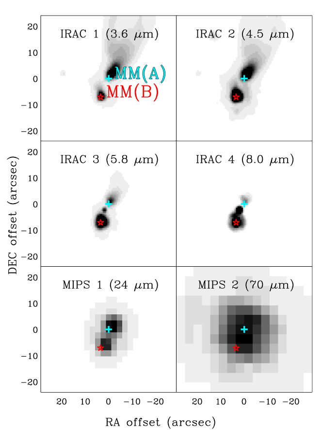
Figure 1: Spitzer images of L1448-MM. Images are $\sim$ 50 $\arcsec$ ($\sim$ 11000 AU) on each side. The cross shows the location of the millimeter emission peak of L1448-MM(A) and the star represents the location of L1448-MM(B). (Jørgensen et al., 2007)

In the IRAC images, the trail of sources aligns in the SE-NW direction (Fig. 1), which is consistent with the large-scale outflows. There is an additional point-like source between L1448-MM(A) and MM(B) in the IRAC band 3 and 4 images, which has been reported as a tertiary 1.3 mm continuum source (Maury et al., 2010). Owing to decreased resolution in MIPS band 2, L1448-MM(A) and MM(B) are not resolved in that image, although they seem distinct from each other in images at shorter wavelength. Hereafter, we designate L1448-MM(A) and L1448-MM(B) as MM(A) and MM(B), respectively.

3.2 The IRS and PACS spectra

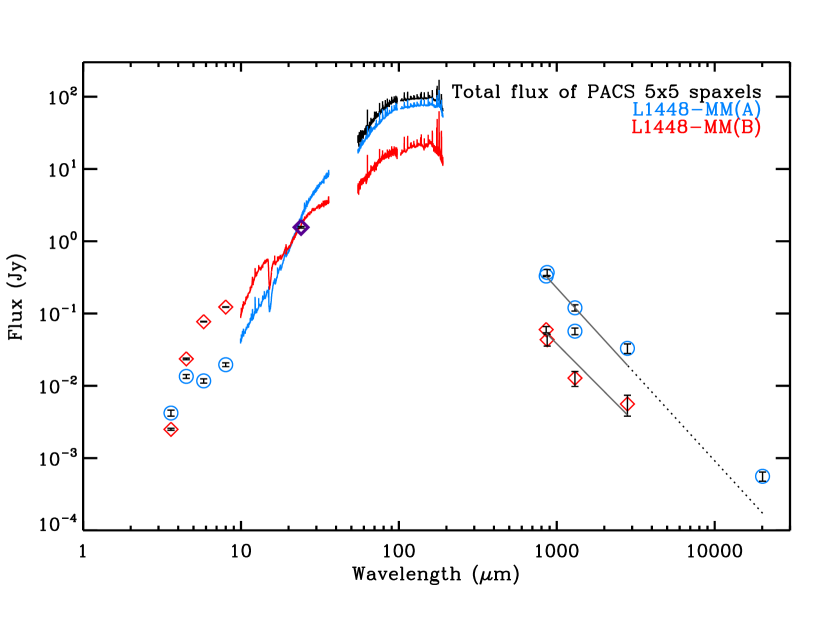
Figure 2: The SEDs of MM(A) and MM(B). The color lines represent spectroscopic observations: The blue lines show spectra from MM(A) in the range of IRS and PACS. The red lines represent spectra from MM(B) in the range of IRS and PACS. The black line displays the spectrum extracted the whole 5 $\times$ 5 array of PACS. The longer than 100 $\mu$m of the PACS spectra has been scaled down by the factor of 0.753 to match the continuum levels around 100 $\mu$m (Green et al. in prep.). Points show millimeter and IR photometry observations: blue circles and red diamonds display MM(A) and MM(B) fluxes, respectively. Purple diamond represents flux at 24 $\mu$m, where MM(A) and MM(B) are not separated. The solid lines present the results of fitting the fluxes in the range of 700 $\mu$m $<$ $\lambda$ $<$ 3000 $\mu$m. The fitted line for MM(A) is extended to $\lambda$ $\sim$ 20000 $\mu$m as a dotted line.

Here we present the SEDs of two point sources, MM(A) and MM(B) collected for wavelengths ranging from a few microns to sub-mm. In Fig. 2, the IR data points come from Jørgensen et al. (2006) and fluxes at millimeter wavelengths are taken from Curiel et al. (1990), Jørgensen et al. (2007), Maury et al. (2010), and Hirano et al. (2010). The IRS spectra of MM(A) and MM(B) are also plotted in Fig. 2.

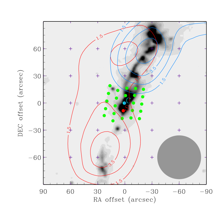
Figure 3: PACS footprint (green) against the IRAC 2 image and the SRAO CO J $=$ 2–1 outflow map. The spaxels located at the positions of MM(A) and MM(B) are designated as spaxels C (blue) and S (red), respectivlely. The purple crosses are the positions of SRAO observation. A much higher resolution map of CO J = 2 – 1 can be found in Bachiller et al. (1990), but the general feature is the same. The grey circle shows the beam FWHM of SRAO. The blue contours are integrated from $-10.0$ to $-1.2$ km s^-1, while the red contours are integrated from 9.9 to 20 km s^-1. The contours start at 1.5 K km s ^-1 and increase by 0.5 and 1.0 K km s^-1 for blue and red components, respectively.

In the PACS range (Fig. 2), the black line represents the spectrum extracted from all 25 spaxels (see §2.1) while the blue and red lines show the spectra of MM(A) and MM(B), separately. All three spectra (black, blue, and red) have been extracted from the HIPE v6.1 reduction, which provides superior flux calibration. In the PACS footprint, MM(A) and MM(B) are located near the central spaxel and the spaxel in the right south of the central spaxel, which are designated as spaxel C and S, respectively, as seen in Fig. 3. The coordinates of spaxel C are the same as the coordinates of MM(A), but the coordinates of spaxel S, (3^h25^m39.0^s, +30^∘43′56.8″), are slightly different from those of MM(B).

To obtain the spectra of MM(A) and MM(B), we 1) extracted spectra from the spaxels, C and S, respectively, 2) scaled to match continuum levels around 100 $\mu$m, and 3) corrected for the effect of the Point Spread Function (PSF) of PACS to each source.

Since the spectra of each segment ($\lambda\sim$50-75, 70-105, 100-145, 140-210 $\mu$m) are not matched smoothly, we scaled up or down SEDs of each segment to match continuum levels around 100 $\mu$m. The scale factors applied to the spectrum extracted from spaxel C are 1.052, 0.918, and 0.854 in the range of $\lambda$ $<$ 72, 101 $\sim$ 142, and $>$ 142 $\mu$m, respectively. The scale factors for the spectrum extracted from spaxel S are 0.903, 0.667, and 0.727, in the same wavelength range.

In order to correct for the PSF, that is, to decompose fluxes of MM(A) and MM(B), we assume that only two point-like sources contribute the emission in the two spaxels and calculate the contribution of each source to the normalized fluxes of two spaxels using the point spread function. The contribution of a point source to the spaxel where it is located is 80 $\%$ at 50 $\mu$m and 32 $\%$ at 200 $\mu$m, and to the adjacent spaxel is $\sim$ 3.5 $\%$ at 50 $\mu$m and $\sim$10 $\%$ at 200 $\mu$m. As a result, at a given wavelength, the fluxes of the two point sources are decomposed by solving two simple linear simultaneous equations as below.

$$F_{\lambda,\rm C}=P_{\lambda,\rm AC}*X_{\lambda,\rm A}+P_{\lambda,\rm BC}*X_{\lambda,\rm B}$$ (1)

$$F_{\lambda,\rm S}=P_{\lambda,\rm AS}*X_{\lambda,\rm A}+P_{\lambda,\rm BS}*X_{\lambda,\rm B}$$ (2)

$F_{\lambda,\rm C}$ and $F_{\lambda,\rm S}$ are fluxes measured from the spectra extracted at spaxel C and S, while $X_{\lambda,\rm A}$ and $X_{\lambda,\rm B}$ are the decomposed fluxes of MM(A) and MM(B), respectively. $P_{\lambda,\rm AC}$ and $P_{\lambda,\rm BC}$ are the contribution to spaxel C by MM(A) and MM(B), while $P_{\lambda,\rm AS}$ and $P_{\lambda,\rm BS}$ are the contribution to spaxel S by MM(A) and MM(B), respectively. $P_{\lambda,\rm AC}$, $P_{\lambda,\rm BC}$, $P_{\lambda,\rm AS}$, and $P_{\lambda,\rm BS}$ were calculated with the exact coordinates of MM(A) and MM(B).

The slope of the SEDs (rising into the FIR) demonstrates that cold material is present showing that both MM(A) and MM(B) are deeply embedded. The continuum luminosity integrated in the PACS wavelength range is about 3.5 and 0.9 $L_{\sun}$ for MM(A) and MM(B), respectively, as listed in Table 4. The bolometric luminosities of MM(A) and MM(B), which are calculated with their decomposed SEDs, are $\sim$5.5 and 1.7 $L_{\sun}$ (see §5).

In the IRS range, the flux of MM(B) is flatter than that of MM(A) longward of 15 $\mu$m. In the IRS spectrum of MM(B), the flux drops shortward of 15 $\mu$m. The excess flux in the IRAC bands compared to what is extrapolated from the IRS SED might be attributed to some shocked gas and scattered light around MM(B).

A deep CO₂ 15.2 $\mu$m ice absorption feature has been detected in both MM(A) and MM(B) (Fig. 4), indicative of the existence of dense envelopes in both sources. Both CO₂ absorption profiles show the broad red wing, which is attributed to the CO₂ and H₂O ice mixture. Although the S/N ratio is somewhat low, we see clearly a double-peaked feature, indicative of the pure CO₂ ice component, which exists only toward protostars (Pontoppidan et al., 2008). In the millimeter wavelength range (700 $<$ $\lambda$ $<$ 3000 $\mu$m), the spectral index ($-d$log$S_{\nu}$/$d$log$\nu$, where $S_{\nu}$ is the flux density, and $\nu$ is the frequency) is about 2.4 for MM(A) and 2.2 for MM(B). These large ($>2$) positive values imply that the millimeter continuum emission comes from dust, not from ionized gas. These SEDs and the CO₂ ice absorption feature, including the pure CO₂ ice feature, indicate that both sources are deeply embedded YSOs. The available millimeter data, however, do not constrain the dust properties further.

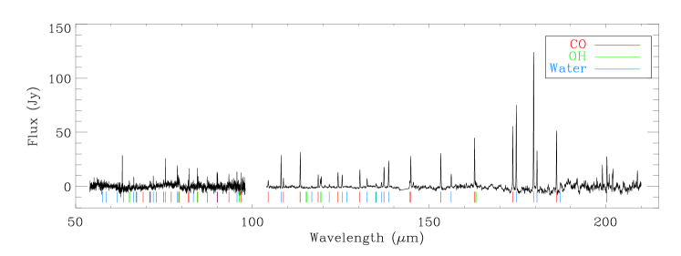
Figure 5: Herschel/PACS continuum-subtracted spectra extracted from all 25 spaxels. The emission lines are marked: CO (red dashes), and OH (green dashes), H₂O (blue dashes).

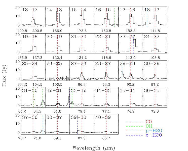
Figure 6: CO emission lines (red vertical dashed lines) detected in L1448-MM. These spectral line are determined from the central spaxel spectrum, in order to present all detected line transitions. Emission lines of other species located close to the CO lines are also marked with different colors (green for OH, blue for p-H₂O, and dark blue for o-H₂O). The rotational transition of each line is noted on the upper left side of each box. The J$=$13–12 line has an artificially lower flux due to a factor of $\sim$ 2 decrease in sensitivity at the edge of the PACS array, and this line is not used in subsequent models.

The PACS spectra show numerous molecular lines of CO, H₂O, and OH in addition to atomic [O I] lines (Fig. 5). The detected lines are listed in Table 1 including the upper level energy, $E_{\rm u}={E_{\rm upper}\over k}$ ($k$ is Boltzmann constant), and the Einstein coefficient, $A_{\rm ul}$. The detected lines of each species are presented in Fig. 6 to  9, where we present lines extracted only from the central spaxel. As the central spaxel contains most of the continuum, many lines were detected only at the central spaxel. Dionatos et al. (2009) calculated a visual extinction ($A_{\rm V}$) of 11 and 32 mag toward MM(A) and MM(B), respectively, using the 9.7 $\mu m$ silicate absorption feature of the IRS spectra. These $A_{\rm V}$ values attenuate line fluxes by less than 10 % at $\lambda\geq 60$ $\mu m$. Therefore, we did not correct for the reddening in line fluxes.

CO transitions were detected from J = 13–12 up to J = 40–39. The highest OH transition is ${}^{2}\Pi_{1/2}$ J = 9/2 – 7/2. Both lines of [O I] at 63 $\mu$m and 145 $\mu$m and 22 ortho- and 19 para-H₂O lines were detected. No H${}_{2}^{18}$O or ¹³CO lines were detected. The upper limits of H${}_{2}^{18}$O (2₁₂-1₀₁) and ¹³CO (15–14) are 1.70 $\times$ 10^-17 and 1.73 $\times$ 10^-17 W m^-2, respectively. Assuming $[^{16}\rm O]/[^{18}\rm O]=550$ and $[^{12}\rm C]/[^{13}\rm C]=90$, the upper limits of optical depth of ¹²CO (15–14) and H${}_{2}^{16}$O (2₁₂-1₀₁) are about 3 and 8, respectively, in the assumption of equal excitation temperatures for the isotopologues.

3.3 The PACS and IRS maps; distribution of continuum and line emission

Figure 3 compares the infrared image in the Spitzer IRAC band 2 with the SRAO CO J $=$ 2–1 outflow map. The footprint of PACS is marked on the image. The IRAC 2 image shows a jet-like structure along a NW and SE path. The SRAO CO J$=$2–1 outflow falls along this axis. The jet-like structure is more prominent to the NW in the IRAC 2 image. Nisini et al. (2000) noted that the adjacent area of the southern lobe has a higher visual extinction than that of northern lobe.

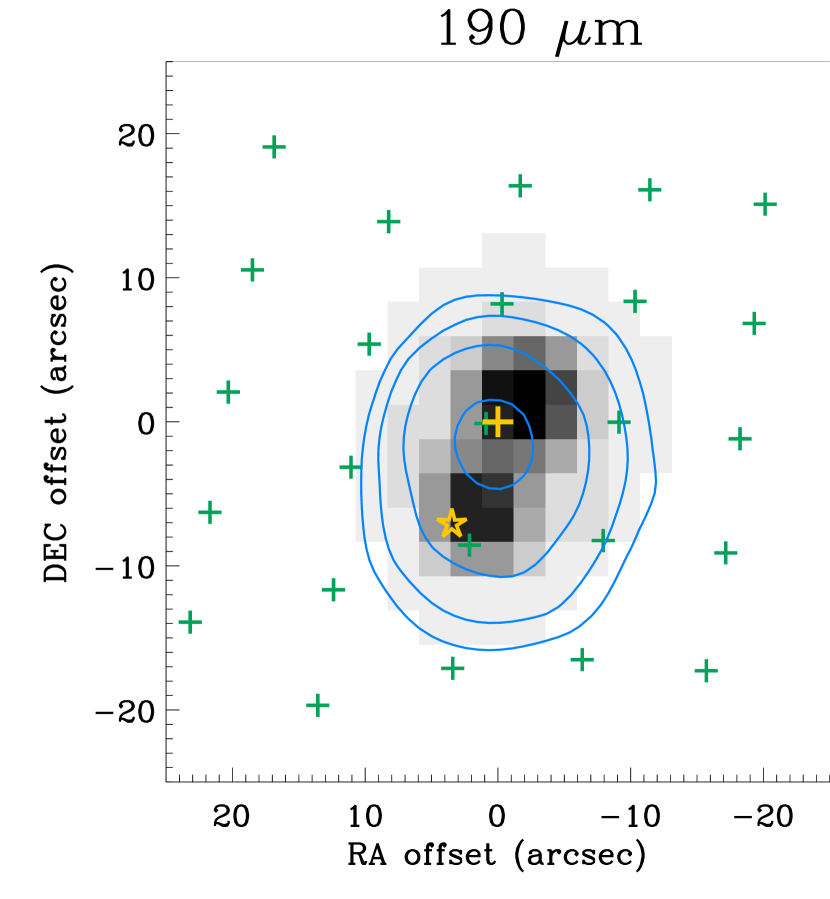
Figure 10: The contour maps of continuum emission at 67 $\mu$m and 190 $\mu$m on top of the MIPS 1 (grey image). In each map, contour levels are 20, 30, 50, and 90 $\%$ of the peak flux. The crosses indicate the locations of the 5 $\times$ 5 spaxels. The sub-mm positions of MM(A) and MM(B) (Jørgensen et al., 2006) are marked as yellow cross and star, respectively.

Figure 10 shows the distribution of continuum emission at 67 $\mu$m and 190 $\mu$m, extracted from the PACS data cube, compared to the MIPS 1 image. The continuum peaks close to MM(A) and slightly extends to MM(B), which is probably due to the contribution of MM(B) in the dust continuum. These two sources were decomposed into the continuum emission as described in section 3.2.

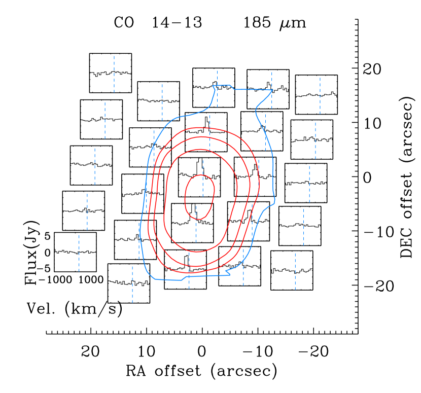
Figure 11: Left: The contour map of the CO J $=$ 34 – 33 line flux on top of its spectrum map. The upper level energy is 3279 K. Right: The same map but for CO J $=$ 14 – 13. The upper level energy is 580 K. The red contour levels are 20, 30, 50, and 90 $\%$ of the peak flux, but one more blue(right) contour is for 10 $\%$ of the peak flux to present the extended emission better.

From Fig. 11 to Fig. 15, the maps of selected lines are presented. In each figure, a contour map is overlaid on the spectral map. Two transitions are selected for each species to study the spatial variation in the emission lines depending on energy level or wavelength; lines representing higher energy levels concentrate on spaxel C while lines of lower energy levels peak 4$\sim 5\arcsec$ toward the south. In addition, the low energy lines tend to distribute more broadly compared to lines from high energy levels. CO (J$=$14–13, 186 $\mu$m), OH (${}^{2}\Pi_{3/2}$ J = 5/2 – 3/2, 119 $\mu$m), o-H₂O (J${}_{K_{-1},K_{1}}$ = 2₁₂–1₀₁, 179 $\mu$m), p-H₂O (J${}_{K_{-1},K_{1}}$ = 3₁₃ – 2₀₂, 138 $\mu$m), and [O I] (${}^{3}P_{1}-^{3}P_{2}$, 63 $\mu$m) are the most evident examples of the spatially broadened distribution. The broad distribution of line emission at longer wavelengths could be real or the effect of the larger PSF at longer wavelengths. Nevertheless, the distribution of [O I] emission appears to be significantly different from the other species as the line flux of the southernmost spaxel is as strong as that at the spaxel S, indicating a relatively flat emission profile over several spaxels.

The line emission does not necessarily correspond to continuum sources spatially. However, the line emission (except for [O I] lines) is the strongest at the spaxels C and S as is the continuum emission. In addition, the peaks of the contour maps both in continuum and line emission are shifted to the south of MM(A) similarly. Therefore, the line emission might originate from two unresolved gas components located at spaxels C and S. In order to test this idea, we decomposed the line fluxes with the same method as used in the decomposition of the continuum (§3.2) by assuming that two unresolved gas components are located at the same positions of MM(A) and MM(B), which is not necessarily true. The decoupled line fluxes are listed in Table 1. Interestingly, the sum of the decomposed molecular line fluxes is consistent with the total fluxes over 25 spaxels within errors while the total [O I] 63 $\mu$m flux over 25 spaxels is greater than the sum of the decomposed fluxes by a factor of $\sim$ 2. Therefore, for CO, OH, and H₂O, the extended emission beyond these two spaxels is mostly caused by the PSFs of the two unresolved gas components while [O I] emission is indeed extended. Fig. 15 also shows the elongated emission along the outflow direction, which indicates that the extended [O I] emission is connected to the outflow.

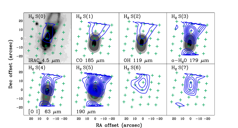
Figure 16: The contour maps (blue) of the H₂ rotational transitions superimposed on spitzer 4.5 $\mu$m image or PACS contour maps of CO, OH, o-H₂O, [O I], and 190 $\mu$m continuum emission (gray scale). PACS contours have levels of 0.2, 0.3, 0.5, 0.9 times of the peak flux. H₂ contours start at 10^-21 W cm^-2 and increase by 10^-21 W cm^-2.

Fig. 16 presents IRS line maps of the rotational transitions of H₂ compared with PACS emission lines and the IRAC 4.5 $\mu$m image. The H₂ emission is not spatially coincident with the FIR emission. H₂ emission is detected primarily from the blue-shifted outflow to the north, where $n$(H₂) is higher and $A\rm_{V}$ is lower (Nisini et al., 2000; Dionatos et al., 2009), while the extended [O I] emission seems to originate from the position of the red-shifted outflow to the south. Therefore, this overall feature of the MIR and FIR emission suggests that the outflow source is located rather close to the surface of the associated molecular cloud. As a result, the column density of shocked material in the blue component is not large enough to block the MIR emission while the column density of shocked material in the red component is large enough to obscure the MIR emission and to produce the strong FIR emission line.

4 Analysis

In order to understand the physical conditions of the gas emitting the detected FIR lines, we utilize two analysis methods: the rotational diagram and the non-LTE Large Velocity Gradient (LVG) code, RADEX. The rotational diagram has been conventionally adopted to provide rough idea of a temperature, which is called rotational temperature and used to explain the relative observed line intensities of a molecular species. However, the LVG analysis can provide more detailed physical conditions such as the kinetic temperature, which is not always the same as the rotation temperature, and the density of the gas.

4.1 Rotational diagrams

This simple excitation analysis assumes that the lines are optically thin. If the populations can be fitted with a single line, the level populations can be characterized by a single temperature ($T_{\rm rot}$). In the case of LTE, $T_{\rm rot}$ is the same as the kinetic temperature of the gas. A detailed description for this rotation diagram can be found in Green et al. (2013) as well as Goldsmith & Langer (1999). In order to produce rotational diagrams, we used the total flux over 25 spaxels as well as the decomposed fluxes for the two unresolved gas components (accidentally) located at the positions of MM(A) and MM(B). The two unresolved gas components are designated as (A) and (B) hereafter. (Here, we note again that the two gas components, (A) and (B) are not necessarily associated with two continuum sources, MM(A) and MM(B).)

The ISO beam and the HIFI beam were too big to resolve (A) and (B) at all. However, due to the much better resolution of PACS, we could decompose the fluxes of (A) and (B) to produce the rotation diagrams for both gas components separately. The errors of the total flux extracted from the whole 25 spaxels are listed in Table 1 while those of the decomposed fluxes are assumed to be 20% of the fluxes. Since we do not know the actual emitting area of each molecule, we use the total number of molecules ($\mathcal{N}$) instead of column density. The results of our rotational diagram analysis are summarized in Table 2.

4.1.1 CO

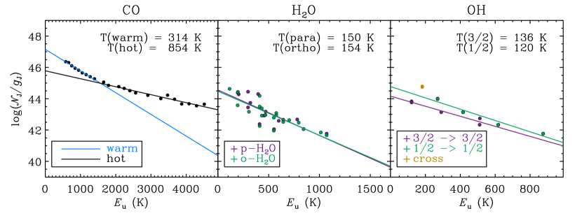
Figure 17: CO, H₂O, and OH rotation diagrams with the total fluxes, in units of total number of detected molecules $\mathcal{N}$ divided by degeneracy g. Left: the CO rotation diagram shows two distinct populations with a break around 1500 K in energy. Center: H₂O rotation diagram. p-H₂O and o-H₂O are fitted separately (purple and green are for p-H₂O and o-H₂O, respectively.). Right: In the OH rotation diagram, two ladders are fitted separately (purple is for ${}^{2}\Pi_{3/2}$, and green is for ${}^{2}\Pi_{1/2}$).

The rotational CO ladder seems to contain a break at $\it E\rm_{u}$ $\sim$ 1500 K (Fig. 17). Therefore, we fitted the rotational diagram with two components. High-J CO lines ($\it E\rm_{u}$ $>$ 1500 K) are fitted by $\it T\rm_{rot}$ of 750–850 K and $\mathcal{N}$(CO) $\sim 6\times$ 10⁴⁸ for the total fluxes and the fluxes of (A) while they are fitted by a lower $\it T\rm_{rot}$ of $\sim$ 450 K with $\mathcal{N}$(CO) $\sim 3\times$ 10⁴⁸ for the fluxes of (B). (According to Green et al. (2013), the break position between the two component does not much affect the result.) Low-J CO lines ($\it E\rm_{u}$ $<$ 1500 K) are fitted by a $\it T\rm_{rot}$ of $\sim$ 300 K for the total fluxes measured over all 25 spaxels, as well as for the fluxes of (A). In contrast, the fluxes of (B) are fitted by a lower $\it T\rm_{rot}$ of $\sim$ 250 K. (The difference in the rotation temperature between (A) and (B) is much greater than the fitting errors.) Therefore, the gas at (A) seems hotter than the gas at (B). The total numbers of CO molecules for this warm component are much greater than those for the hot component; $\mathcal{N}$(CO) $\sim$ 2.8$\times$ 10⁴⁹, 1.6$\times$ 10⁴⁹, and 1.4 $\times$ 10⁴⁹ for the total fluxes, (A), and (B), respectively (see Table 2).

The warm (T$\sim$300 K) and hot (T$\sim$1000 K) CO gas components have been explained by a combination of PDRs and shocks (Visser et al., 2012). According to the scenario, the UV radiation from the central object can heat the outflow cavity walls up to 300$\sim$400 K, but shocks are necessary to heat the gas to emit at high-J CO transitions of $\it E\rm_{u}$ $>$ 1500 K. However, recent PACS surveys of YSOs (Manoj et al., 2013; Karska et al., 2013) show that the UV heating along the cavity wall is a minor contributor to the excitation of the FIR CO fluxes. In addition, a more self-consistent 2-D PDR model developed by Lee et al. (in prep.) also shows that the UV heated outflow cavity wall cannot produce the rotational temperature of 300 K, which is universally fitted by the PACS low-J CO lines ($\it E\rm_{u}$ $<$ 1500 K), especially in Class 0 sources. Therefore, shocks seem to be the predominant heating source in these embedded YSOs.

4.1.2 H₂O

Because of the different possible orientations of the spins of H atoms, H₂O has two kinds of states, ortho- and para-H₂O; in equilibrium above a threshold ambient temperature and critical density, the ratio of degeneracies of states is 3:1, accounting for the state degeneracies. Compared to CO and OH, H₂O shows increased scatter in its rotational diagram (Fig. 17), probably because the water lines are usually sub-thermal due to their high critical densities or have different opacities.

For the rotational diagram based on the full array fluxes, the o-H₂O transitions are fitted by $\it T\rm_{rot}$ = 144 $\pm$ 5 K and $\mathcal{N}$(H₂O) = (2.4 $\pm$ 0.3) $\times$ 10⁴⁶ while p-H₂O transitions are fitted by $\it T\rm_{rot}$ = 168 $\pm$ 6 K and $\mathcal{N}$(H₂O) = (6.2 $\pm$ 0.9) $\times$ 10⁴⁵. We also separated (A) and (B) in the rotational diagram, and the results are listed in Table 2. The rotational temperatures calculated from water lines are much lower than those calculated from CO lines. If two species coexist in the same physical conditions, the derived rotational temperatures indicates the sub-thermal conditions of water lines. Therefore, in order to study the physical conditions of the gas associated with water lines, we have to utilize a non-LTE calculation.

In (A) and (B), $\mathcal{N}$(o-H₂O)/$\mathcal{N}$(p-H₂O) is greater than 2. Considering the optical depth effect, it is not very different from 3. Therefore, this may indicate that water formed at a temperature high enough for H₂O to be in spin equilibrium, or the timescale is long enough to equilibrate the ortho-to-para ratio of water after it evaporates from grain surfaces. The rotation temperature for (A) is higher than (B), consistent with our results from CO in the previous section.

4.1.3 OH

The spin-orbit interaction of OH results in two separate ladders of rotational levels denoted as follows: ${}^{2S+1}\Lambda_{J}=$ ${}^{2}\Pi_{1/2}$ and ${}^{2}\Pi_{3/2}$. Each rotational level is split by $\Lambda$ doubling and hyperfine structure (Offer et al., 1994). In the PACS spectra, typically the transitions between different $\Lambda$ doublet levels are resolved while the hyperfine structure is not resolved, although in some cases even the ladder transitions are blended. When the total fluxes extracted from $5\times 5$ spaxels are used, lines in the ${}^{2}\Pi_{3/2}$ ladder are fitted to $\it T\rm_{rot}$ = 115 $\pm$ 9 K with $\mathcal{N}$(OH) = 7.6 $\pm$ 2.0 $\times$ 10⁴⁵, while the ${}^{2}\Pi_{1/2}$ transition lines are fitted to $\it T\rm_{rot}$ = 114 $\pm$ 7 K with $\mathcal{N}$(OH) = 4.0 $\pm$ 1.3 $\times$ 10⁴⁵ (Fig. 17). Two ladders have different y-intercepts in the rotational diagram, and $\mathcal{N}$(${}^{2}\Pi_{1/2}$)/$\mathcal{N}$(${}^{2}\Pi_{3/2}$) is $\sim$0.6, suggesting that OH lines may not be optically thin, or the OH gas is not thermalized. (The ratio of partition functions of the two ladders is $\sim 0.15$ at $T=115$ K.) Non-thermal effects might contribute to OH emission lines if the OH lines are optically thin.

According to Wampfler et al. (2010), radiative pumping via the cross ladder transitions is more important in the population of the ${}^{2}\Pi_{1/2}$ levels while transitions in the ${}^{2}\Pi_{3/2}$ ladder are mostly excited by collisions. To test the idea, we produced an LVG model including the FIR continuum radiation from the central source as a non-thermal effect. The result is presented in next section. We also fitted line fluxes for (A) and (B), separately as done for CO and H₂O. However, the number of OH lines for (B) is not large enough for a meaningful fitting. The results are summarized in Table 2.

4.2 RADEX models of CO, H₂O, and OH emission

According to the rotation diagrams, the gas component (A) located at the central spaxel has higher rotational temperatures and total molecular numbers compared to the gas component (B) located at the spaxel, S. However, the rotational diagrams cannot provide detailed information on kinetic temperatures and densities of the two gas components. In addition, we know that those spatially distinct gas components have different kinematical components based on earlier studies (Bachiller et al., 1990; Dutrey et al., 1996; Nisini et al., 2000; Kristensen et al., 2011; Nisini et al., 2013) although our PACS spectrum does not resolve the complex kinematics.

Therefore, we used a non-LTE LVG model, RADEX (van der Tak et al., 2007), to connect different physical conditions to the two spatially distinct components. In the model, the level populations are determined by three physical parameters: the gas temperature $T\rm_{K}$, the H₂ density $n$(H₂), and the column density of a molecule divided by the line width, $\Delta v$. With RADEX, we explore a wide range of physical conditions to interpret observed line ratios. For molecular data, the LAMDA database (Schoier et al., 2005) was used (Offer et al., 1994; Faure et al., 2007; Yang et al., 2010).

First, we upgraded RADEX with the subroutine, “newt” (Press et al., 1992; Yun et al., 2009), which is a globally used convergent Newton method, because the downloadable RADEX code sometimes does not easily converge to the solution for H₂O and OH lines. Second, for the OH and H₂O molecules, we tested the importance of radiative pumping by replacing a part of the cosmic background radiation with a blackbody radiation field emitted from the inner boundary of the envelope: $BACK=W\times BB\rm(T)+\it(1-W)\times BB\rm{(2.7K)}$ where $BB\rm(T)$ is the Planck function of temperature $T$, and $W$ is the filling factor of an inner source. Kristensen et al. (2011) adopted the inner boundary temperature of 250 K from Jørgensen et al. (2002) for their best-fit envelope model of L1448-MM with a power-law density structure described with $n=n_{0}\times(\frac{r}{r_{0}})^{-1.5}$ ($n_{0}$ = 1.3 $\times$ 10⁹ cm^-3, $r_{0}$ = 20.7 AU). (The temperature at the inner boundary is not well constrained because it has been derived based on the continuum at the wavelengths of 60 $\mu$m to a few millimeters, which is dominated by the outer cold envelope.) We assumed that the radiation emitted from the inner boundary of the envelope traveled through the outflow cavity to reach a position in the outflow cavity wall without much attenuation. If we assume a characteristic density at the position where the radiation lands, the radius ($r$) from the center to that position can be found from the envelope density profile. Therefore, $W=(1-cos\theta)\times(1/2)$, where $\theta=sin^{-1}(r_{0}/r)$, assuming a spherical central radiation source. Finally, the observed intensity is $I=[BB(T\rm_{ex})-\it BB\rm(2.7K)]\times(1-\it exp(-\tau))$, where $T\rm_{ex}$ and $\tau$ are the excitation temperature and the optical depth for each transition, respectively; we assumed that the infrared source is not located along the line-of-sight when deriving line fluxes since the contribution of the flux affected by the IR source (through absorption) to the total flux within a spaxel is negligible.

4.2.1 CO

According to the rotation diagram, CO fluxes of both (A) and (B) seem to require multiple gas components, so we tested three combinations of physical components of gas (one gas component, two gas components, and the gas with a power-law temperature distribution) in order to check whether the non-LTE calculation also shows the same conclusion. We fitted the observed PACS fluxes of (A) and (B), separately, assuming that all gas components contribute to the total flux equally. In this test, we adopted the line width (60 km s^-1) of the broad component, which was detected in the HIFI observations (Kristensen et al., 2011) and contributed dominantly to the HIFI fluxes. In order to find the best model, we compared flux ratios since we do not know the actual size of the line emitting source. We scaled total model flux to total observed flux and calculated reduced $\chi^{2}$. The best-fit models for three different combinations of gas conditions are summarized in Table 3.

According to Neufeld (2012), the PACS CO data can be fitted by one component with a high temperature ($T\rm_{K}\sim$ 3000 K) and low density ($n\sim$ 10^4-5 cm^-3). However, the modeled rotation diagram of (A) with one component shows lower curvature compared to the observed one although the CO fluxes of (B) seems fitted well with the gas model with $T\rm_{K}=$ 4000 K and $n=$ 10⁴ cm^-3 (See Fig. 18).

The two gas components can fit better the CO fluxes of both (A) and (B); the two temperatures for (A) are both 5000 K while the two temperatures for (B) are 5000 K and 2000 K. In the model with a power-law temperature distribution, (A) and (B) have a similar power index, b ($\sim 3$), but the density for (A) is about 4 times higher compared to (B). This test shows that multi-components of gas can explain better the fluxes of both (A) and (B), and the high temperatures derived from the LVG models indicates shock origin.

4.2.2 H₂O

We also tested the three different combinations of gas components for the H₂O lines adopting the line width of 50 km s^-1, which is the velocity of the broad component detected by (Kristensen et al., 2011), for all components. As for CO lines, the two-component model fits better than the single component model for both (A) and (B) although the single component model still fits the observed fluxes reasonably. In the single component model, (A) requires a higher kinetic temperature (2000 K) than (B) (700 K) while the density for (A) is lower than that for (B). The best-fit model with a power-law temperature distribution for (A) has $b=0$, indicative of hot gas components are dominant emitter for the water lines. However, the $\chi^{2}$ of this model is much worse than one or two components model because this model assumed that all lines are optically thin. The parameters for these best-fit models are summarized in Table 3.

4.2.3 OH

For OH, we fitted fluxes only of (A) since the majority of emission is from spaxel C, except for the 119 $\mu$m doublet. In addition, the collision rates for OH are available only up to $T=300$ K. As a result, we modeled OH fluxes with a single physical component.

We explored models within the following parameter space: 50 $<T<250$ K, $10^{3}<\it n(\rm H_{2})<1.3\times 10^{9}$ cm^-3, and 5$\times 10^{11}<N(\rm OH)<5\times 10^{17}$ cm^-2. We assumed a line width of 50 km s^-1, which is appropriate for the broad component of H₂O gas (Kristensen et al., 2011). Since it has been suggested that the FIR radiation field can play an important role in the excitation of OH, we included it in our model, as described in the first part of this section. Although we considered only attenuated emission from the central source as the FIR radiation source without considering the FIR radiation from the surrounding material in situ, the model including the effect of the FIR radiation in the OH excitation can fit the observed fluxes better.

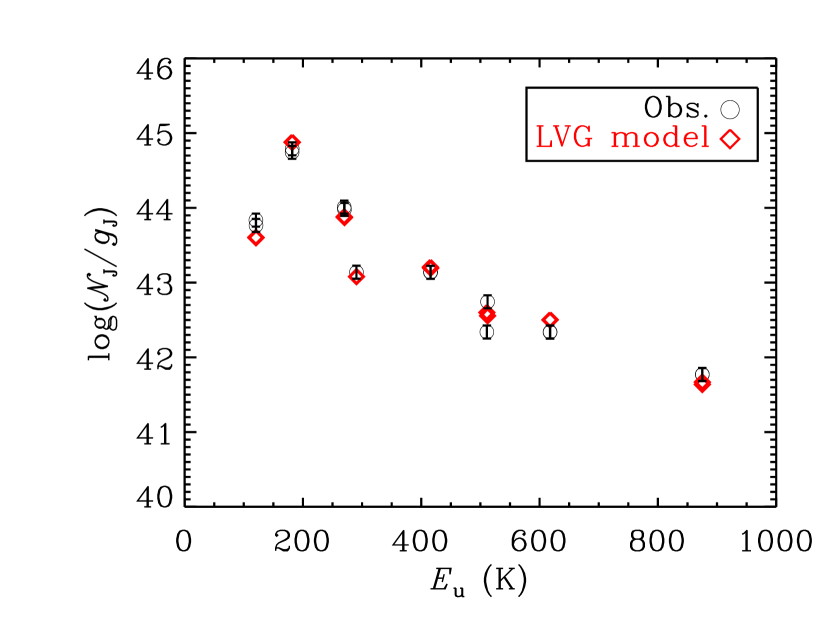
Figure 20: The best models of OH in (A). The circles represent observed fluxes while the red diamonds display model fluxes. Left: the best-fit LVG model with the IR-pumping effect included ($\chi^{2}\sim 4.7$). The observed fluxes can be well fitted when the central IR radiation is considered in the OH level populations. Right: the same model as the best-fit model but excluding the IR radiation effect ($\chi^{2}\sim 6.9$). The line flux at the observed highest energy level is underproduced in the model without IR-pumping.

Fig. 20 (left) presents our best-fit OH model, where the FIR radiation plays a role in the excitation of OH. In the model, the temperature is 125 K, the H₂ density is 2$\times$10⁸ cm^-3, and the OH column density is 5$\times$10¹⁷ cm^-2. As described in the very first part of this section, this density would be reached at a radius of 72 AU in the adopted 1-D density profile. Therefore, the 250 K blackbody radiation field is diluted to the position of the envelope. To examine the effect of FIR radiation on OH fluxes, we compared the same model without the FIR radiation effect in Fig. 20 (right). At lower energy levels, the radiation effect is not prominent, but it makes a significant difference at the highest energy level transition; the flux at the highest energy level ($E_{\rm u}=$ 875 K) in the model with IR-pumping is greater by a factor of 5 compared to the flux derived from the model without IR-pumping.

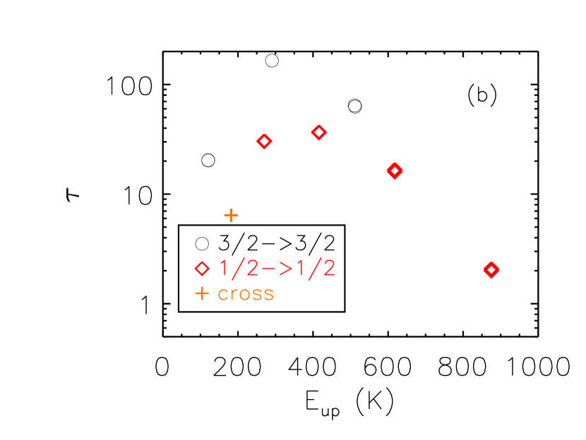
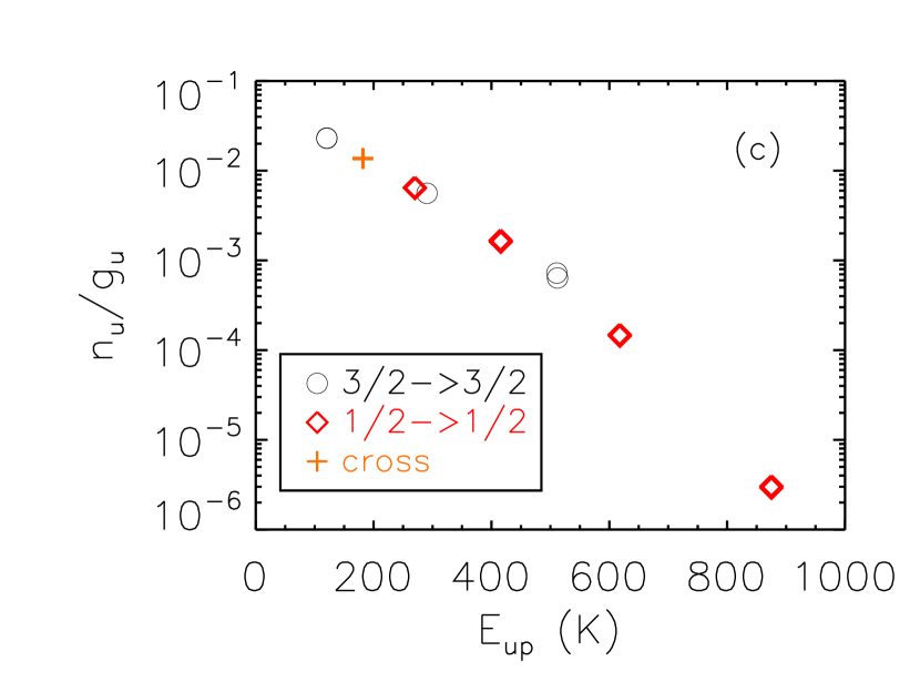
Figure 21: The excitation temperature (a), optical depth (b), and level population (c) of each line in the best-fit OH model with IR-pumping for (A). The blue dashed line in (a) indicates the kinetic temperature of this model. In (c), the upper level population is divided by the statistical weight of the upper level.

Although the IR effect is important for the high energy level transition, the overall fluxes are not affected much. The difference between y-intercepts of ${}^{2}\Pi_{3/2}$ and ${}^{2}\Pi_{1/2}$ ladders, therefore, in the rotational diagram should have other causes. Fig. 21 shows the excitation temperature and optical depth of each transition in the best-fit model. The kinetic temperature of the model is marked as a red dotted line in the left box. All transitions are sub-thermal, and ${}^{2}\Pi_{3/2}$ lines are extremely optically thick compared to ${}^{2}\Pi_{1/2}$ transitions. Therefore, the higher optical depth of ${}^{2}\Pi_{3/2}$ compared to ${}^{2}\Pi_{1/2}$ results in the separation (i.e., different y-intercepts) of two ladders in the rotational diagram, where a constant temperature ($T_{\rm rot}$) and the optically thin case are assumed. Fig. 21(c) shows the actual level populations of the best-fit model, which results in equal populations for the two spin states. Therefore, the separation of two ladders in the rotational diagram is caused both by optical depth effect and IR-pumping.

4.3 Comparison with Shock Models

Based on the ISO observations, Nisini et al. (2000) concluded that the CO, H₂O, H₂, and [O I] IR emission in L1448-MM is caused by a non-dissociative shock with a low velocity, and the kinetic temperature of the shocked gas is about 1200 K. The CO and H₂O line profiles are also very broad (FWHM$\sim 50$ km s^-1), strongly suggesting that the associated gas is related to shocks (Kristensen et al., 2011; Nisini et al., 2013). In addition, interferometric observations and analysis of the EHV features in L1448-MM show that they are likely jet-shock features (Hirano et al., 2010). Therefore, the derived excitation conditions and resolved kinematical components infer that shocks play an important role in L1448-MM.

The shocks produced by the interaction between the outflow and the envelope heat the gas, resulting in emission. Since the shock could dissociate the gas in the dense envelope, which consists mainly of molecular gas, the shock could change relative abundances among the species H₂, H, O, CO, and H₂O. Therefore, the relative intensities of these emission lines are indicative of the type and speed of the shock waves and of the physical conditions in the gas. We compared our line fluxes to the calculation by Flower & Pineau des Forêts (2010) for both C- and J-shocks. In the comparisons, we consider a single physical component for all the emission. The calculations by Flower & Pineau des Forêts (2010) cover shock velocities from 10 to 40 km s^-1 (the shock with 40 km s^-1 is only for the C-shock) and hydrogen densities $n(\rm H)$ of 2 $\times$ 10⁴ $\sim$ 2 $\times$ 10⁵ cm^-3. The magnetic field strength in the pre-shock gas is given as $b[n(\rm H)(cm^{-3})]^{1/2}\mu$G, with $b$ = 1 in the C-shock and $b$ = 0.1 in the J-shock.

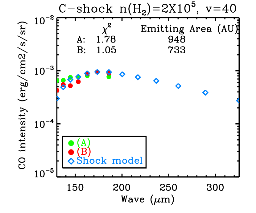
Figure 22: Comparisons of observed CO line fluxes with shock model fluxes (left for the best-matched C-shock model and right for the best-matched J-shock model.) T he model parameters of density and velocity are presented at the top of boxes. $\chi^{2}$ and the emitting areas to fit the observed fluxes are presented inside boxes.

The relative CO line fluxes of (A) are well matched by the J-shock model with $n{\rm(H_{2})}$ = 2$\times 10^{4}$ cm^-3 and $v$ = 20 km s^-1. The C-shock model with $n{\rm(H_{2})}$ = 2$\times 10^{5}$ cm^-3 and $v$ = 40 km s^-1 also reproduces the observed line flux ratios reasonably well. In the case of (B), the relative line fluxes are well fitted by the C-shock model with $n{\rm(H_{2})}$ = 2$\times 10^{5}$ and $v$ = 40 km s^-1 (Fig. 22). The diameter of emitting areas derived from these models are about 1000$\sim$2000 AU.

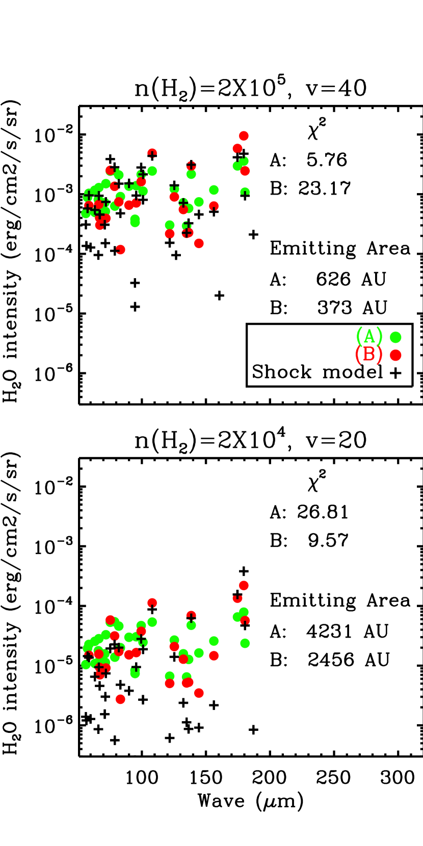
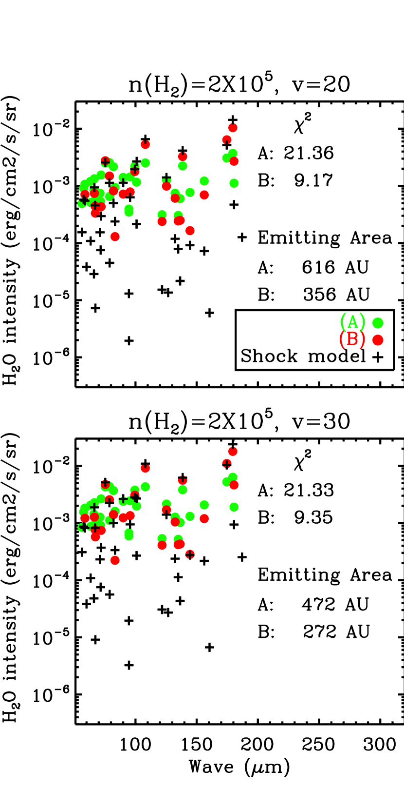
Figure 23: The same plot as Fig. 22 but for H₂O (left for the best-matched C-shock models and right for the best-matched J-shock models.)

The relative H₂O line fluxes of (A) are well matched by the C-shock model with $n{\rm(H_{2})}$ = 2$\times 10^{5}$ cm^-3 and $v$ = 40 km s^-1. For (B), the C-shock model with $n{\rm(H_{2})}$ = 2$\times 10^{4}$ cm^-3 and $v$ = 20 km s^-1 and the J-shock model with $n{\rm(H_{2})}$ = 2$\times 10^{5}$ cm^-3 in $v$= 20 km s^-1 and 30 km s^-1 fit well the observed flux ratios (Fig. 23). When we consider that H₂O line fluxes are highly scattered, (B) can be also explained by the shock model for (A). In that case, the relative fluxes of CO and H₂O at both (A) and (B) are reproduced by the C-shock model with $n{\rm(H_{2})}$ = 2$\times 10^{5}$ and 40 km s^-1, supporting the idea that H₂O and CO are excited at the same physical conditions as suggested in Karska et al. (2013).

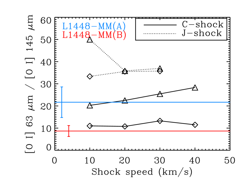
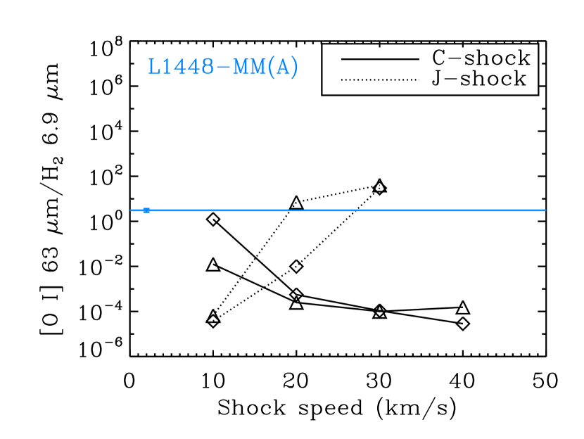
Figure 24: The line flux ratios as a function of shock conditions (Flower & Pineau des Forêts, 2010). The shock parameters are the shock speed (km s^-1) and preshock H₂ density (cm^-3). Solid lines and dashed lines represent C- and J-shock models, respectively. Diamonds refer to 2 $\times$ 10⁴ cm^-3 and triangles to 2 $\times$ 10⁵ cm^-3 of hydrogen density. Horizontal lines indicate the values of L1448-MM and vertical lines represent the uncertainties. Blue and red colors represent the flux ratios for (A) and (B), respectively. Left: The line flux ratio of [O I] 63 $\mu$m to 145 $\mu$m. Right: The line intensity ratios of [O I] 63 $\mu$m with respect to H₂ S(5) 6.9 $\mu$m pure rotation transition. H₂ fluxes are convolved with PACS spaxels.

Due to its low upper level energy of 230 K, the [O I] 63 $\mu$m line is easily excited, and thus, it is an important cooling channel in the postshock region. As a result, it is one of the best tracers of shocks in dense environments (Giannini et al., 2001). We calculated the [O I] 63/145 $\mu$m ratio for (A) and (B), which are $\sim$ 22 and 9, respectively. In (A), flux ratio corresponds to low density C-shock model while flux ratio of (B) fits to a high density C-shock model as seen in Fig. 24 (left). Therefore, the flux ratios of [O I] lines are consistent with the C-shock model.

However, the [O I] flux is severely under-estimated by the C-type shock models; an emitting region of $>10^{4}$ $\times$ 10⁴ AU², corresponding to $>50$ spaxels, would be required. Alternatively, more than 50 individual shocks would be required to generate this amount of emission. If a J-shock model is adopted (with $v$ = 30 km s^-1 and $n{\rm(H_{2})}$ = 2$\times 10^{4}$ cm^-3 for (A) and 2$\times 10^{5}$ cm^-3 for (B)), the emitting area is 300 $\times$ 300 AU² (1/40 spaxel) for (A) and 400 $\times$ 400 AU² (1/25 spaxel) for (B). Considering the spatial distribution of the [O I] emission covering more than four spaxels (Fig. 15), neither a single C-shock nor a single J-shock can reproduce the [O I] absolute fluxes and extent, indicative of multiple shock components.

Flower & Pineau des Forêts (2010) also calculated several H₂ line strengths under the same shock conditions and compared the intensities with those of [O I] emission. In (A), the ratio is fitted to a J-shock model with shock speed of 20–30 km s^-1 and a low density C-shock model with $v\rm_{shock}$ $<$ 20 km s^-1 simultaneously (Fig. 24). In (B), however, the observed fluxes cannot be compared with the model flux ratios since the H₂ fluxes avoids the (B) position. Therefore, the ratio of [O I] to H₂ emission could not constrain the shock characteristics in (B).

These comparisons suggest that a C-shock model can explain most of emission in L1448-MM, but the [O I] absolute fluxes and the [Si II] emission detected in the IRS spectra indicate that a dissociative J-shock should also exist in this region. According to Neufeld & Dalgarno (1989), [Si II] emission cannot be produced by a non-dissociative shock, but could be produced by either a dissociative shock or PDR. The dissociative shock tracers such as [Si II] and [Fe II] often go close together with non-dissociative shock tracers (e.g., Neufeld et al. (2009)), and the dissociative apex of a bow shock that is flanked by non-dissociative shocks is suggested to explain this feature. Therefore, we cannot designate a single type of shock in the simple planar models for L1448-MM; we require more sophisticated multi-dimensional shock models with different initial conditions to explain the relative emission of each species in this complicated region.

4.4 Luminosities

Table 4 presents luminosities for the lines detected in L1448-MM as well as continuum. The total line luminosity accounts for only $\sim$ 0.7% of the total FIR luminosity in the PACS range. Therefore, the dominant cooling occurs by the continuum radiation. According to Nisini et al. (1999) and Giannini et al. (2001), the FIR line luminosities of L1448-MM calculated from the ISO observations are greater than what we derive from our PACS observations by factors of 2 to 8 depending on species although the relative luminosities among different species are similar. However, ISO and PACS both show that the line cooling mainly occurs through H₂O emission. In contrast, the FIR continuum luminosity obtained by ISO is much smaller than what derived by PACS by a factor of 20, resulting in a higher fraction of line luminosity to the continuum luminosity in FIR. These differences in luminosities between ISO and PACS are probably caused by the low sensitivity and large beam of ISO compared to PACS. In L1448-MM, molecular emission extends beyond the FOV of PACS. Therefore, the ISO beam, larger than the PACS FOV, possibly picked up a significant amount of the extended molecular emission.

In the PACS line luminosity, CO, H₂O, and OH emission arises mostly from (A); $\sim 70\%$ of the total CO and H₂O fluxes are emitted from (A), while (B) supplies $\sim 30\%$ of the CO and H₂O line cooling, and most of OH line emission ($\sim 90\%$) is concentrated on (A). However, the sum of [O I] line luminosity of (A) and (B) has just $\sim 65\%$ of the total luminosity calculated over the whole 5$\times$5 spaxels, indicative of broadly extended emission in [O I]. If we assume that the gas components of (A) and (B) are associated with MM(A) and MM(B), respectively, the ratio of the FIR line luminosity in the PACS range to the bolometric luminosity ($L_{\rm mol}/L_{\rm bol}$) both for MM(A) and MM(B) is $\sim 4\times 10^{-3}$, indicating that both sources are in the Class 0 stage. According to Giannini et al. (2001), $L_{\rm mol}/L_{\rm bol}>1\times 10^{-3}$ for Class 0 objects while the ratio is smaller than $5\times 10^{-4}$ for Class I and II sources. According to our best-fit LVG models, H₂O and CO emit the majority ($>50-80\%$) of their luminosity in the PACS wavelength range.

Table 5 shows the fractional contribution of each species to the FIR line luminosity as a total and in (A) and (B). van Dishoeck et al. (2011) suggested that H₂O might not be the dominant coolant in YSOs. For L1448-MM, however, water is the primary outflow coolant and this is consistent with the results for the Class 0 protostar NGC 1333 IRAS 4B (Herczeg et al., 2012), where H₂O is responsible for 72% of line luminosity. H₂O occupies $\sim 50\%$ and CO fills $\sim 30\%$ of the line luminosity in the PACS wavelength range in L1448-MM. For CO, the warm ($E\rm_{u}<$ 1500 K) and hot ($E\rm_{u}>$ 1500 K) components are responsible for $\sim$65% and $\sim$35% of the CO line luminosity in the PACS range, respectively, based on the results of rotation diagrams. OH and [O I] contribute $\sim$ 10% and $\sim$ 5% of the line luminosity, respectively. In L1448-MM, the cooling through molecular emission is significantly larger than the cooling via atomic emission, which is consistent with the characteristic of the Class 0 YSOs (Nisini et al., 2002; Herczeg et al., 2012). Bright H₂O emission and dim [O I] emission in L1448-MM is indicative of low dissociation rate of H₂O, or the fast formation process of H₂O in the postshock gas. Alternatively, [O I] and H₂O emission possibly arises from unassociated gas components, i.e., the [O I] emission is attributed to a more extended gas while the H₂O emission is localized around the YSOs.

5 Discussion

5.1 Multiple Sources in L1448-MM

Previously, L1448-MM was known as a single YSO with a prominent outflow. However, Jørgensen et al. (2007), Tobin et al. (2007), and Hirota et al. (2011) suggested the existence of a secondary YSO, named L1448-MM(B) while Maury et al. (2010) suggested that the secondary point-like source at Spizer bands and 3 mm might be a result of a shock on the outflow cavity wall. However, we conclude that L1448-MM(B) is a YSO based on its millimeter SED (Fig. 2) and the detection of the double peak structure of CO₂ ice absorption feature at 15.2 $\mu$m (Fig. 4) (Pontoppidan et al., 2008).

The SEDs (Fig. 2) of MM(A) and MM(B) rising into the FIR indicate that both sources are very embedded. Hirano et al. (2010) suggested that MM(B) was likely less obscured in the MIR compared to MM(A). This is consistent with a much higher FIR flux level in MM(A) than in MM(B), indicating less material toward MM(B). From the separated SEDs and the photometric data points in Green et al. (2013), we calculated the bolometric luminosities ($L_{\rm bol}$) of MM(A) and MM(B) as 5.5 and 1.7 $L_{\sun}$, respectively, which do not add up to $L_{\rm bol}$ of 8.4 $L_{\sun}$ calculated over the whole region (Green et al., 2013). For the calculation, single-dish (sub)millimeter fluxes for two sources were separated based on the flux ratios derived from the interferometric observations. (The interferometric continuum fluxes were not included in the calculation of $L_{\rm bol}$ and $T_{\rm bol}$ although they do not affect the results at all.) The derived $L_{\rm bol}$ for each source is rather sensitive to this flux separation at (sub)millimeter. Therefore, it should not be considered very accurate. The calculated bolometric temperatures ($T_{\rm bol}$) of MM(A) and MM(B) are 49 and 80 K, respectively, indicating that MM(A) is more embedded and in the earlier evolutionary stage. $L_{\rm bol}/L_{\rm smm}$ are 18.7 and 48.7 for MM(A) and MM(B), respectively, which also suggests that MM(A) is more embedded. Note that MM(B) is classified as Class I by ($T_{\rm bol}$) but Class 0 by $L_{\rm bol}/L_{\rm smm}$ while MM(A) is classified as Class 0 by both criteria.

MM(A) is separated from MM(B) by 8$\farcs$17 that is equivalent to $\sim$2000 AU. Mundy et al. (2001) divided embedded multiple systems into three groups: independent envelope, common envelope, and common disk systems. As seen in the submm continuum maps (Shirley et al., 2000), two sources seem associated with only one dense core. Therefore, L1448-MM may be a common envelope system which has one primary core in gravitational contraction, and where objects are separated by 250 – 3000 AU. Although the possible detection of the CO₂ gas line at 14.98 $\mu$m (Dartois et al., 1998) toward MM(A) is indicative of a hotter region, the column density of CO₂ ice, calculated from the IRS 15.2 $\mu$m CO₂ ice feature, is $\sim$2 $\times$ 10¹⁸ cm^-2 in both YSOs. This might also support the idea that they are in a common envelope.

5.2 Shocked Gas in L1448-MM

The outflow activity in the two sources appears significantly different. Hirano et al. (2010) has reported that the weak CO outflow possibly associated with MM(B) is nearly perpendicular to that of MM(A), and its small momentum flux is comparable to those of outflows by Class I objects. However, the MM(A) outflow elongates in the SE-NW direction. Since MM(B) is about $8\arcsec$ south of MM(A), fluxes in spaxel S are likely contaminated by the outflow emission from the MM(A). The continuum emission of MM(A) is greater than that of MM(B) at $\lambda\geq 20$ $\mu$m. Lines of high energy levels also peak in the position of MM(A) while the emission peaks of lines of lower energy levels shift to the south. These features suggest that MM(A) may be the primary outflow source in the direction of SE-NW. Then the gas traced in our PACS observations may be heated predominantly by the jet/outflow driven by MM(A). If this is true, the molecular gas in (A) and (B) rather correspond to the blue and red wings of the L1448-MM(A) jet, which were detected by the CO and SiO transitions (Nisini et al., 2000; Hirano et al., 2010).

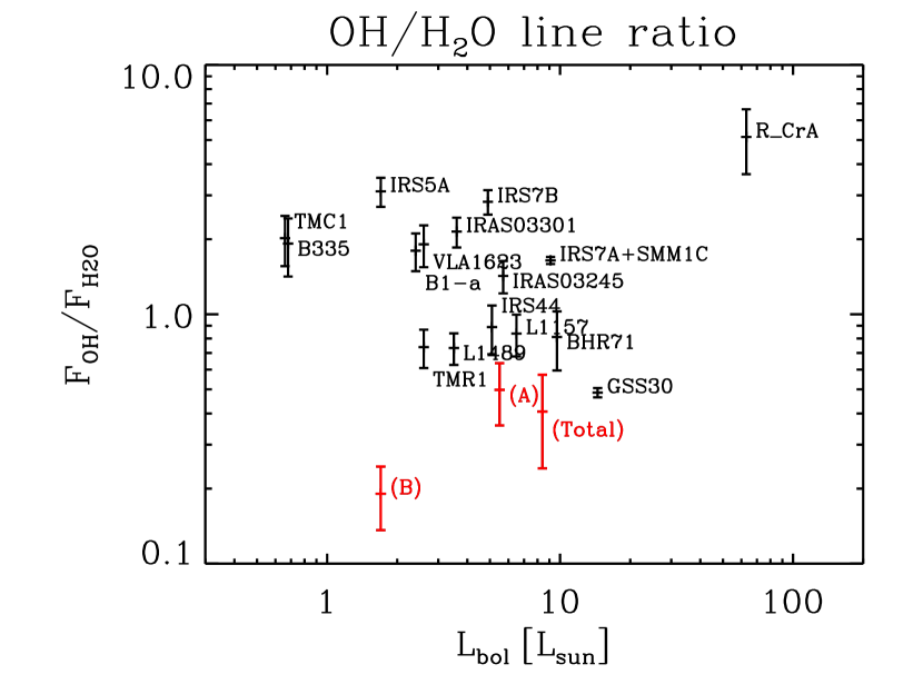
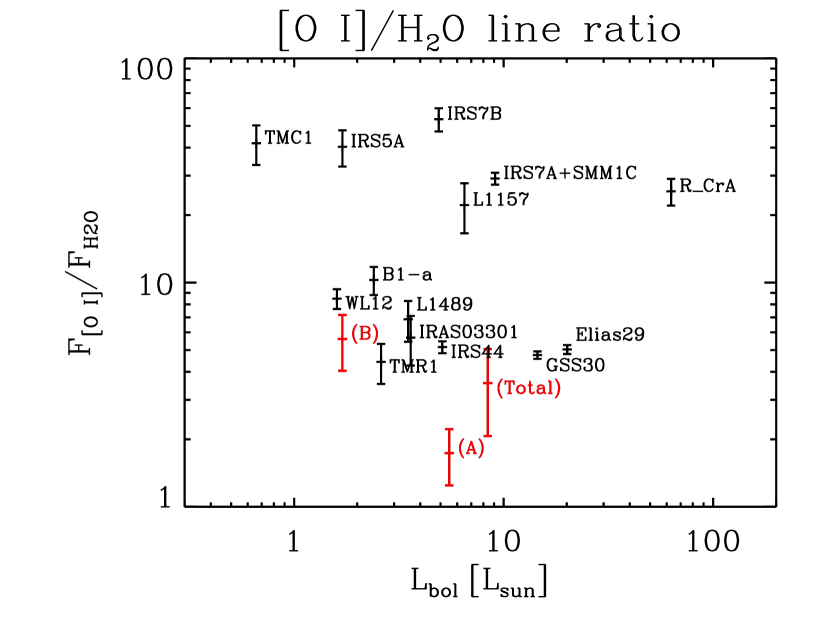
Figure 25: OH and [O I] line fluxes relative to H₂O line flux toward the DIGIT embedded sources (Green et al., 2013). Left: the flux ratio of the OH (84 $\mu$m, $E_{\rm u}$ = 291 K) and the o-H₂O (75 $\mu$m, $E_{\rm u}$ = 305 K) Right: The flux ratio of the [O I] (63 $\mu$m, $E_{\rm u}$ = 227 K) and o-H₂O (66 $\mu$m, $E_{\rm u}$ = 410 K). The minimal ratios for L1448-MM indicate that the photodissociation is not important in the region.

According to our excitation analyses of (A) and (B), the PACS FIR line fluxes are possibly produced mainly by shocked hot gas components, rather than by the UV-heated gas along the outflow cavity. According to (Yildiz et al., 2010), up to J=10–9, the contribution of the broad wing component increases with J, hinting that shocks may play a more important role in higher J transitions traced by the PACS. However, if the UV photons play an important role in this region, we should expect an enhancement of the [O I] and OH line fluxes compared to H₂O. In order to check the relative emission among [O I], OH, and H₂O, as done in Lindberg et al. (subm.), we calculated the flux ratios between the OH (84 $\mu$m, $E_{\rm u}$ = 291 K) and o-H₂O (75 $\mu$m, $E_{\rm u}$ = 305 K) lines, which have small PSFs and similar upper-level energies, as well as the flux ratios between [O I] (63 $\mu$m, $E_{\rm u}$ = 227 K) and o-H₂O (66 $\mu$m, $E_{\rm u}$ = 410 K) lines, toward the DIGIT embedded sources (Fig. 25). According to the comparisons, L1448-MM has the minimum flux ratios among the DIGIT embedded sources, supporting that the observed line emission in L1448-MM is mainly from shocks.

Comparing to the recently observed Class 0 objects, NGC 1333 IRAS4B (hereafter, IRAS4B) and Serpens SMM1(hereafter, SMM1), L1448-MM is similar to IRAS4B in molecular emission; water dominates in the line cooling and [O I] is dim. In addition, the best model for IRAS4B with the non-LTE analysis suggests the physical conditions of $T_{\rm K}\sim$1500 K and $n(\rm H_{2}$) $\sim$3$\times$10⁶ cm^-3. In SMM1, however, CO is the main coolant and [O I] is relatively brighter than the other two sources, and the derived physical conditions are $T_{\rm K}\sim$800 K and $n(\rm H_{2})\geq$ 5$\times$10⁶ cm^-3. Therefore, the derived physical conditions for L1448-MM are more similar to those of IRAS4B. In addition, [C II] (158 $\mu$m) is detected in SMM1 but not detected in IRAS4B and L1448-MM. $L_{\rm OH}$/$L_{\rm H_{2}O}$ of L1448-MM and IRS4B are $\sim$0.2 while that of SMM1 is 0.4. $L_{\rm OI}$/$L_{\rm H_{2}O}$ are 0.06$\sim$0.1, 0.01, and 0.6 for L1448-MM, IRS4B, and SMM1, respectively. (Goicoechea et al. (2012) mentioned that the strong [O I] and OH emission towards SMM1 is similar to that of HH46, a Class I source (van Kempen et al., 2010a).) Therefore, the FIR line emission in L1448-MM and NGC 1333 IRAS4B might have a similar origin, i.e., non-dissociative shocks shielded from UV radiation play a larger role in the excitation than dissociative shocks (Herczeg et al., 2012).

6 Summary $\&$ Conclusion

Contour maps show that FIR line emission from low energy levels is toward the south while H₂ emission in the MIR peaks toward the north. Most of FIR molecular line emission is from the unresolved two gas components, (A) and (B), both of which might be heated by the jet shock of MM(A). For CO and H₂O ($L_{\rm CO}+L_{\rm H_{2}O}$), $\sim 70\%$ of cooling occurs in (A) while most OH emission ($\sim 90\%$ of $L_{\rm OH}$) concentrates on (A). Differently from other species, the [O I] emission extends more broadly beyond the two positions to the south.

According to the simple rotational diagram model, CO seems to have two temperature components (warm and hot), which have been attributed by previous studies to the PDR and shock, respectively. The rotational temperatures and total number of molecules of the two CO components in (A) are higher than those measured in (B). This tendency is true for OH and H₂O as well. Therefore, the gas in (A) is hotter and has more of the excited molecules than does (B), according to the rotation diagram analysis. In the case of H₂O, the derived ortho-to-para ratio is close to 3, indicating that H₂O might have formed in the hot postshock gas, or the timescale is long enough to equilibrate the ortho-to-para ratio of water after its evaporation from grain surfaces. For OH, $\mathcal{N}$(${}^{2}\Pi_{1/2}$)/$\mathcal{N}$(${}^{2}\Pi_{3/2})\sim$0.6, which is greater than the ratio of partition functions of the two ladders by a factor of 4 at 115 K. This is possibly due to the IR-pumping in the ${}^{2}\Pi_{1/2}$ transitions and/or higher optical depths of the ${}^{2}\Pi_{3/2}$ transitions.

According to our non-LTE LVG analyses, the PACS CO and H₂O emission arises from shocked gas (rather than photo-heated gas) and requires multiple gas components with different physical conditions.

The non-LTE LVG model shows the sub-thermal condition of OH. All OH lines except the highest energy level ($E_{\rm u}=$ 875 K) transition are optically thick, and the optical depths of the ${}^{2}\Pi_{3/2}$ transitions are higher than those of the ${}^{2}\Pi_{1/2}$ transitions. Therefore, the displacement between two ladders in the rotation diagram is caused by the higher optical depths of the ${}^{2}\Pi_{3/2}$ transitions. In addition, the LVG model supports the IR-pumping processes for OH transitions because the OH line flux of $E_{\rm u}=$ 875 K is much better fitted when the FIR radiation from the central source is included. In contrast, the IR-pumping is not very important for the H₂O lines.

Our best-fit LVG models predict that (50–80)% of the molecular line emission is produced in the PACS wavelength range depending on models. The continuum luminosity observed in the PACS range is $\sim$ 50% of $L\rm_{bol}$. The modeled cooling luminosities are $L_{\rm CO}\sim(1.1-2.4)\times 10^{-2}$ $L_{\sun}$ and $L_{\rm H_{2}O}\sim(2.0-4.5)\times 10^{-2}$ $L_{\sun}$ while HIFI observations predict $L_{\rm CO}\sim$ 0.5 $\times 10^{-2}$ $L_{\sun}$ and $L_{\rm H_{2}O}\sim 2-4\times 10^{-2}$ $L_{\sun}$ for CO and H₂O, respectively (Kristensen et al., 2011). Both models show that the major line cooling occurs at the wavelengths $>$ 60 $\mu$m, which is consistent with the ISO result (Nisini et al., 2000).

In comparisons with shock models, the PACS molecular emission can be explained by a C-shock, but the atomic emission such as PACS [O I] and Spitzer/IRS [Si II] requires a J-shock, indicative of multiple shocks in L1448-MM.

In conclusion, our study of L1448-MM with the PACS spectra shows that the atomic and molecular line observations at the FIR wavelengths are very important to understand in detail the energy budget and excitation conditions in the embedded YSOs.

The center of the images corresponds to the coordinates of L1448-MM(A), ($\alpha$, $\delta$)=(3^h25^m38.87^s, +30^∘44′5.4″). The coordinates of L1448-MM(B) are (3^h25^m39.14^s, +30^∘43′58.3″).

Figure 4: The optical depth of the CO₂ 15.2 $\mu$m ice absorption feature toward MM(A) and MM(B). The emission line around 15 $\mu$m in MM(A) is possibly the CO₂ gas line at 14.98 $\mu$m (Dartois et al., 1998). The arrows indicate the double-peaked feature, which is produced by the pure CO₂ ice component.

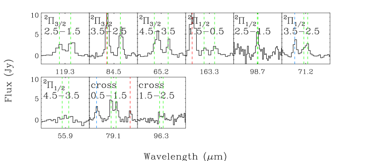
Figure 7: The same as Fig. 6 but for OH lines.

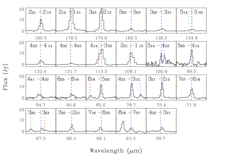
Figure 8: The same as Fig. 6 $\&$  7 but for o-H₂O lines.

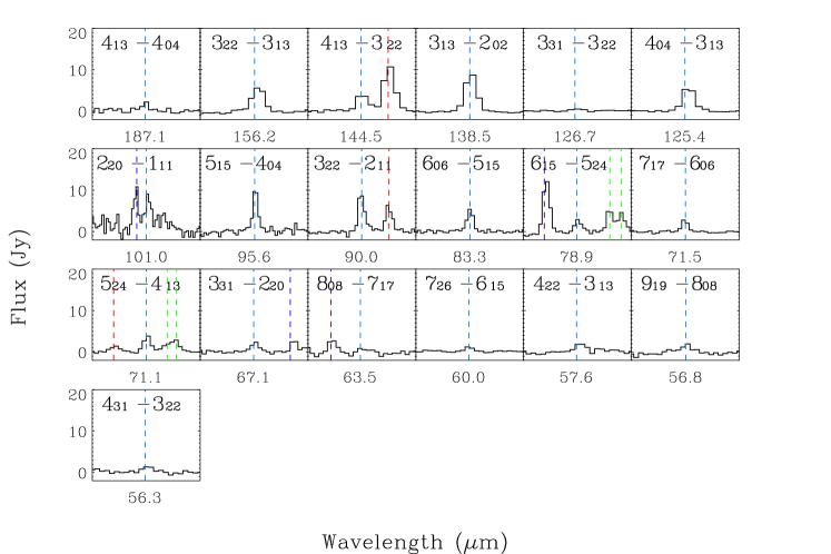
Figure 9: The same as Fig. 6,  7 $\&$  8 but for p-H₂O lines.

Figure 12: Left: The same maps as Fig. 11 but for o-H₂O J${}_{K_{-1},K_{1}}$ = 4₃₂ – 3₂₁. The upper level energy is 550 K. Right: The same map but for o-H₂O J${}_{K_{-1},K_{1}}$ = 2₁₂ – 1₀₁. The upper level energy is 114 K.

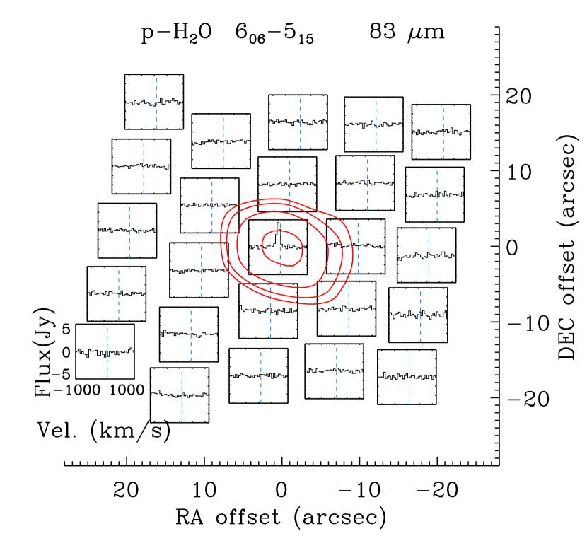
Figure 13: Left: The same maps as Fig. 11 but for p-H₂O J${}_{K_{-1},K_{1}}$ = 6₀₆ – 5₁₅. The upper level energy is 643 K. Right: The same map but for p-H₂O J${}_{K_{-1},K_{1}}$ = 3₁₃ – 2₀₂. The upper level energy is 205 K.

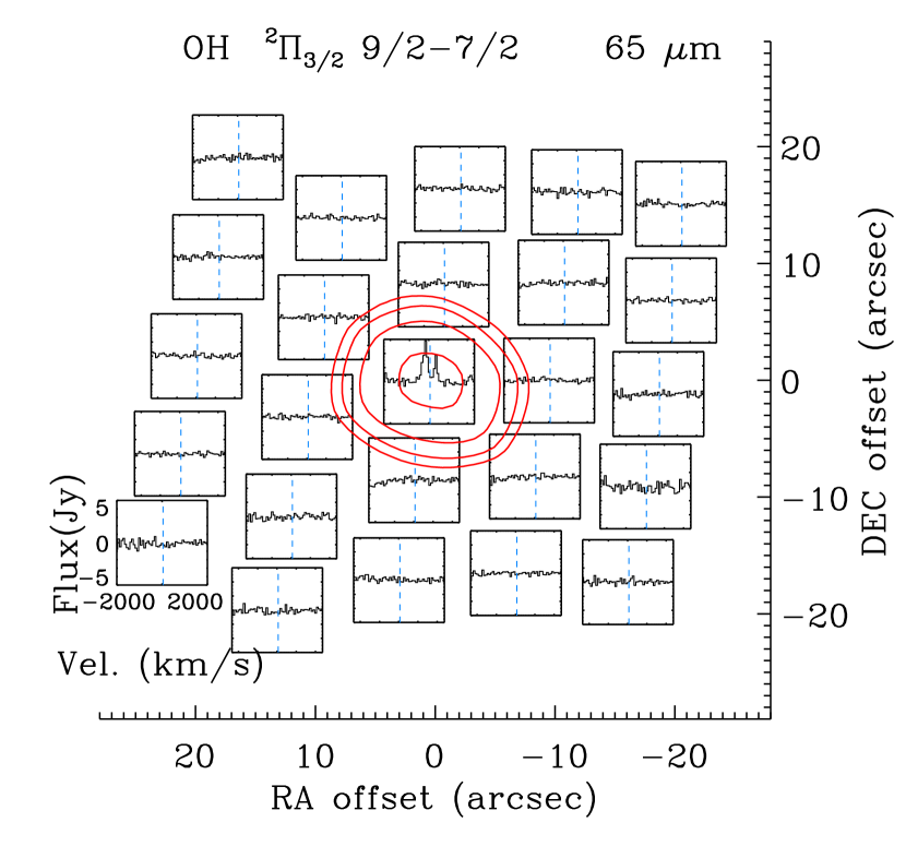
Figure 14: Left: The same maps as Fig. 11 but for OH ${}^{2}\Pi_{3/2}$ J $=$ 9/2 – 7/2. The upper level energy is 512 K for J $=$ 9/2– – 7/2+ and 511 K for J $=$ 9/2+ – 7/2–. Right: The same map but for OH ${}^{2}\Pi_{3/2}$ J = 5/2 – 3/2. The upper level energies are 121 K for both J $=$ 5/2– – 3/2+ and J $=$ 5/2+ – 3/2–.

Figure 15: The same maps as Fig. 11 but for [O I] ${}^{3}P_{1}-^{3}P_{2}$. The upper level energy is 228 K.

Figure 18: The best-fit LVG models for CO lines of (A) (top) and (B) (bottom), respectively. For (B), 84 $\mu$m line is excluded in the fitting. The first column shows one component model, the second column shows two components model, and the third column shows a model with power-law temperature distribution. The reduced $\chi^{2}$ for each model is presented inside boxes.

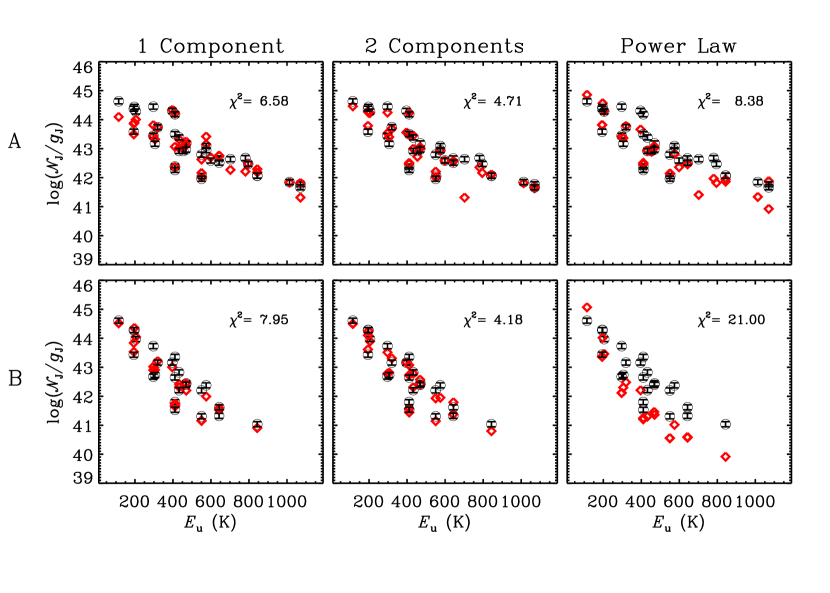
Figure 19: The same as Fig. 18 but for H₂O.

Table 1: Detected lines in Herschel/PACS spectrum of L1448-MM

Species	Transition	$E\rm_{u}$ (K)	$A\rm_{ul}$ (cm-1)	$\lambda$ ($\mu$m)	Flux $(10^{-18}$ W m-2)
					$5\times$5	(A)	(B)
CO	40-39	4512.67	0.00461300	65.69	67$\pm$ 26	77	-
	39-38	4293.64	0.00436500	67.34	60$\pm$ 19	55	-
	38-37	4079.98	0.00412000	69.07	74$\pm$ 22	67	-
	37-36	3871.69	0.00387800	70.91	61$\pm$ 25	58	-
	36-35	3668.78	0.00363800	72.84	104$\pm$ 39	104	-
	35-34	3471.27	0.00340400	74.89	91$\pm$ 27	166	-
	34-33	3279.15	0.00317500	77.06	123$\pm$ 36	88	-
	33-32	3092.45	0.00295200	79.36	83$\pm$ 27	-	-
	32-31	2911.15	0.00273500	81.81	121$\pm$ 36	110	12
	30-29	2564.83	0.00232100	87.19	172$\pm$ 54	117	45
	29-28	2399.82	0.00212600	90.16	214$\pm$ 64	139	40
	28-27	2240.24	0.00194000	93.35	214$\pm$ 65	167	38
	27-26	2086.12	0.00176100	96.77	229$\pm$ 75	182	-
	25-24	1794.23	0.00143200	104.44	195$\pm$ 56	152	59
	24-23	1656.47	0.00128100	108.76	234$\pm$ 68	203	65
	22-21	1397.38	0.00100600	118.58	288$\pm$ 81	217	77
	21-20	1276.05	0.000883300	124.19	328$\pm$ 92	236	90
	20-19	1160.20	0.000769500	130.37	350$\pm$ 99	256	100
	19-18	1049.84	0.000665000	137.20	381$\pm$ 108	259	128
	18-17	944.970	0.000569500	144.78	422$\pm$ 120	294	122
	17-16	845.590	0.000482900	153.27	433$\pm$ 123	300	146
	16-15	751.720	0.000405000	162.81	503$\pm$ 142	318	206
	15-14	663.350	0.000335400	173.63	547$\pm$ 155	373	222
	14-13	580.490	0.000273900	186.00	507$\pm$ 144	303	211
OH	$\frac{1}{2}$,$\frac{9}{2}$-$\frac{1}{2}$,$\frac{7}{2}$	875.100	2.18200	55.89	87$\pm$ 32	70	-
		875.100	2.17500	55.95	88$\pm$ 33	70	-
	$\frac{3}{2}$,$\frac{9}{2}$-$\frac{3}{2}$,$\frac{7}{2}$	512.100	1.27600	65.13	312$\pm$ 96	332	-
		510.900	1.26700	65.28	141$\pm$ 41	129	-
	$\frac{1}{2}$,$\frac{7}{2}$-$\frac{1}{2}$,$\frac{5}{2}$	617.600	1.01400	71.17	100$\pm$ 29	76	13
		617.900	1.01200	71.22	101$\pm$ 29	76	13
	$\frac{1}{2}$,$\frac{1}{2}$-$\frac{3}{2}$,$\frac{3}{2}$	181.900	0.0360600	79.12	190$\pm$ 59	172	26
		181.700	0.0359800	79.18	167$\pm$ 49	154	39
	$\frac{3}{2}$,$\frac{7}{2}$-$\frac{3}{2}$,$\frac{5}{2}$	290.500	0.520200	84.60	251$\pm$ 73	207	29
	$\frac{1}{2}$,$\frac{3}{2}$-$\frac{3}{2}$,$\frac{5}{2}$	270.200	0.00927000	96.31	37$\pm$ 21	-	-
		269.800	0.00925000	96.37	15$\pm$ 17	-	-
	$\frac{3}{2}$,$\frac{5}{2}$-$\frac{3}{2}$,$\frac{3}{2}$	120.700	0.138800	119.23	202$\pm$ 57	124	77
		120.500	0.138000	119.44	249$\pm$ 73	145	102
	$\frac{1}{2}$,$\frac{3}{2}$-$\frac{1}{2}$,$\frac{1}{2}$	270.200	0.0648300	163.12	53$\pm$ 16	46	7
		269.800	0.0645000	163.40	58$\pm$ 17	49	2
p-H2O	431–322	552.300	1.45200	56.33	89$\pm$ 42	81	-
	919–808	1324.00	2.48600	56.77	125$\pm$ 39	-	-
	422–313	454.300	0.378500	57.64	120$\pm$ 37	151	-
	726–615	1021.00	1.33800	59.99	69$\pm$ 24	-	-
	808–717	1070.60	1.74200	63.46	61$\pm$ 23	84	-
	331–220	410.400	1.22200	67.09	137$\pm$ 41	94	24
	524–413	598.800	0.667900	71.07	131$\pm$ 40	123	-
	717–606	843.800	1.17800	71.54	96$\pm$ 28	88	-
	615–524	781.100	0.452600	78.93	96$\pm$ 32	108	-
	606–515	642.700	0.713200	83.28	165$\pm$ 48	156	7
	322–211	296.800	0.352400	89.99	298$\pm$ 95	233	39
	515–404	469.900	0.446000	95.63	276$\pm$ 78	238	43
	220–111	195.900	0.260700	100.98	342$\pm$ 117	-	-
	404–313	319.500	0.172700	125.35	285$\pm$ 81	209	54
	331–322	410.400	0.0784800	126.71	24$\pm$ 8	-	-
	313–202	204.700	0.125100	138.53	520$\pm$ 147	371	181
	413–322	396.400	0.0331600	144.52	124$\pm$ 38	127	9
	322–313	296.800	0.0524600	156.19	239$\pm$ 70	202	38
	413–404	396.400	0.0372600	187.11	32$\pm$ 13	-	-
o-H2O	432–321	550.400	1.37400	58.70	184$\pm$ 53	177	39
	818–707	1070.70	1.75100	63.32	210$\pm$ 67	199	-
	716–625	1013.20	0.950800	66.09	125$\pm$ 43	139	-
	330–221	410.700	1.24300	66.44	259$\pm$ 76	221	41
	330–303	410.700	0.00850500	67.27	127$\pm$ 37	124	18
	707–616	843.500	1.15700	71.95	276$\pm$ 80	257	24
	321–212	305.300	0.331800	75.38	617$\pm$ 176	416	152
	423–312	432.200	0.483800	78.74	522$\pm$ 147	424	82
	616–505	643.500	0.749100	82.03	417$\pm$ 118	359	45
	625–616	795.500	0.174000	94.64	113$\pm$ 32	65	-
	441–432	702.300	0.152800	94.71	68$\pm$ 19	57	-
	505–414	468.100	0.390200	99.49	547$\pm$ 170	366	99
	514–423	574.700	0.156600	100.91	247$\pm$ 90	192	-
	221–110	194.100	0.256400	108.07	735$\pm$ 210	419	296
	432–423	550.400	0.122900	121.72	52$\pm$ 15	52	13
	423–414	432.200	0.0808400	132.41	173$\pm$ 50	123	33
	514–505	574.700	0.0757900	134.93	70$\pm$ 22	50	13
	330–321	410.700	0.0661900	136.50	117$\pm$ 34	99	13
	532–523	732.100	0.0817400	160.51	48$\pm$ 14	-	-
	303–212	196.800	0.0504800	174.63	824$\pm$ 233	510	355
	212–101	114.400	0.0559300	179.53	1173$\pm$ 334	615	579
	221–212	194.100	0.0305800	180.49	337$\pm$ 96	184	149
[O I]	3P1–3P2	227.712	0.0000891	63.18	922$\pm$275	383	230
[O I]	3P0–3P1	326.579	0.0000175	145.53	84$\pm$30	18	26

Note. — Emissions of CO $\&$ OH (84 $\mu$m) and CO $\&$ o-H₂O (113 $\mu$m) are detected, but not measured since they are blended. CO J=13-12 is detected but not included in our analysis because of low responsivity of PACS in this wavelength range.

Table 2: Summary of the rotation diagram analysis

		$5\times$5			(A)			(B)
Species	Component	$T\rm_{rot}$	$\mathcal{N}$(molecule)		$T\rm_{rot}$	$\mathcal{N}$(molecule)		$T\rm_{rot}$	$\mathcal{N}$(molecule)
		(K)	(1047)		(K)	(1047)		(K)	(1047)
CO	Hot	758$\pm$54	65$\pm$19		854$\pm$42	55$\pm$10		455$\pm$37	31$\pm$13
	Warm	293$\pm$30	275$\pm$98		314$\pm$24	164$\pm$41		250$\pm$15	136$\pm$34
H2O	Para	168$\pm$6	0.06$\pm$0.01		150$\pm$5	0.06$\pm$0.01		74$\pm$3	0.06$\pm$0.01
	Ortho	144$\pm$5	0.24$\pm$0.03		154$\pm$4	0.15$\pm$0.02		88$\pm$2	0.13$\pm$0.02
OH	${}^{2}\Pi_{3/2}$-${}^{2}\Pi_{3/2}$	115$\pm$9	0.076$\pm$0.020		136$\pm$9	0.044$\pm$0.008		-	-
	${}^{2}\Pi_{1/2}$-${}^{2}\Pi_{1/2}$	114$\pm$7	0.040$\pm$0.013		120$\pm$4	0.027$\pm$0.005		-	-

Table 3: The best-fit LVG model parameters for three different combinations of gas components

		1 Component				2 Components				Power Law
Species	Spatial	$T\rm_{kin}$	$n(\rm H_{2}$)	$N$(mole)	$\chi^{2}$	$T\rm_{kin}$	$n(\rm H_{2}$)	$N$(mole)	$\chi^{2}$	$n(\rm H_{2}$)	b	$N$(mole)	$\chi^{2}$
	Component	(K)	(cm-3)	(cm-2)		(K)	(cm-3)	(cm-2)		(cm-3)		(cm-2)
CO	A	5000	105	1.9$\times 10^{14}$	2.41	5000	$10^{6}$	1.9$\times 10^{11}$	0.92	2.51$\times 10^{7}$	2.95		1.26
						5000	$10^{4}$	6.0$\times 10^{13}$
	B	4000	104	1.9$\times 10^{18}$	0.67	5000	$10^{4}$	6.0$\times 10^{18}$	0.46	6.31$\times 10^{6}$	3.30		0.73
						2000	$10^{7}$	1.9$\times 10^{16}$
H2O	A	2000	106	6.3$\times 10^{17}$	6.58	100	$10^{5}$	6.3$\times 10^{18}$	4.71	2.51$\times 10^{7}$	0.0	$10^{13}$	8.38
						5000	$10^{8}$	6.3$\times 10^{14}$
	B	700	107	6.3$\times 10^{15}$	7.95	1000	$10^{5}$	6.3$\times 10^{17}$	4.18	6.31$\times 10^{6}$	3.2	$10^{13}$	21.00
						300	$10^{4}$	6.3$\times 10^{16}$
OH	A	125	2$\times$108	5.0$\times 10^{17}$	4.67

Table 4: Luminosities in FIR for the full map and each position

Species	$5\times 5$	(A)	(B)
$L_{\rm CO}$	0.96	0.70	0.27
$L_{\rm H_{2}O}$	1.73	1.21	0.39
$L_{\rm OH}$	0.34	0.30	0.05
$L_{\rm OI}$	0.17	0.07	0.04
$L_{\rm continuum}$	430	349	90

Table 5: Fractional contribution to total line cooling for full map and each position

Species	$5\times 5$	(A)	(B)
$L_{\rm CO}$	30$\%$	31$\%$	36$\%$
$L_{\rm H_{2}O}$	54$\%$	53$\%$	52$\%$
$L_{\rm OH}$	11$\%$	13$\%$	7$\%$
$L_{\rm OI}$	5$\%$	3$\%$	5$\%$

Appendix A Line flux and error calculation

Reduced data with HIPE v6.1 are flux calibrated more accurately while HIPE v8.1 provide higher S/N spectra. Therefore, we calculated equivalent width from HIPE v8.1 reduction $(EW_{8}$) and multiplied the equivalent width by the local continuum of HIPE v6.1 reduction $(F\rm_{conti,6}$) to obtain line flux $(LF)$ over 5$\times$5 spaxels.

$LF=EW\rm_{8}\times\it F\rm_{conti,6}=\rm\frac{\it LF\rm_{8}}{\it F\rm_{conti,8}}\times\it F\rm_{conti,6}$,

where $\it F\rm_{conti,6}$ were measured from a sum over the whole 5$\times$5 spaxels while $EW\rm_{8}$ were measured from the spectrum extracted over only two spaxels (C and S) except for [OI] lines. For the [OI] lines, $EW\rm_{8}$ were measured from the sum over 4 spaxels with clear detection.

According to the error propagation, the line flux errors in Table 1 are calculated with the equation,

$\delta LF=\sqrt{(\frac{F\rm_{conti,6}}{\it F\rm_{conti,8}}\delta\it LF\rm_{8})^{2}+(\frac{\it LF\rm_{8}\times\it F\rm_{conti,6}}{\it F\rm_{conti,8}^{2}}\delta\it F\rm_{conti,8})^{2}+(\frac{\it LF\rm_{8}}{\it F\rm_{conti,8}}\delta\it F\rm_{conti,6})^{2}}$.

We assumed that continuum uncertainty is 20$\%$ of the flux.

References

- Bachiller et al. (1990) Bachiller, R., Martin-Pintado, J., Tafalla, M., et al. 1990, A&A, 231, 174
- Bachiller et al. (1991) Bachiller, R., Andre, P., & Cabrit, S. 1991, A&A, 241, L43
- Bachiller et al. (1995) Bachiller, R., Guilloteau, S., Dutrey, A., et al. 1995, A&A, 299, 857
- Bally et al. (1993) Bally, J., Lada, E. A., & Lane, A. P. 1993, ApJ, 418, 322
- Barsony et al. (1998) Barsony, M., Ward-Thompson, D., & Andre, P. 1998, ApJ, 509, 733
- Bontemps et al. (1996) Bontemps, J., Andre, P., Terebey, S., et al. 1996, A&A, 311, 858
- Chernin (1995) Chernin, L. M. 1995, ApJ, 440, L97
- Claussen et al. (1996) Claussen, M. J., Wilking, B. A., Benson, P.J., et al. 1996, ApJS, 106, 111
- Curiel et al. (1990) Curiel, S., Raymond, J. C., Moran, J. M., et al. 1990, ApJ, 365, L85
- Curiel et al. (1995) Curiel, S., Raymond, J. C., Walfire, M., et al. 1995, ApJ, 453, 322
- Dartois et al. (1998) Dartois, E., d’Hendecourt, L., Boulanger, F., et al., 1998, A&A, 331, 651
- Dartois et al. (1999) Dartois, E., Demyk, K., d’Hendecourt, L., et al. 1999, A&A, 351, 1066
- Dionatos et al. (2009) Dionatos, O., Nisini, B., Lopez, R. G., et al. 2009, ApJ, 692, 1
- Draine et al. (1983) Draine, B. T., Roberge, W. G., & Dalgarno, A. 1983, ApJ, 264, 485
- Dutrey et al. (1996) Dutrey, A., Guilloteau, S., & Bachiller, R. 1997, A&A, 325, 758
- Faure et al. (2007) Faure, A., Crimier, N., & Ceccarelli, C. 2007, A&A, 472, 1029