Shortcut to adiabaticity in internal bosonic Josephson junctions

Abstract

We extend a recent method to shortcut the adiabatic following to internal bosonic Josephson junctions in which the control parameter is the linear coupling between the modes. The approach is based on the mapping between the two-site Bose-Hubbard Hamiltonian and a 1D effective Schrödinger-like equation, valid in the large $N$ (number of particles) limit. Our method can be readily implemented in current internal bosonic Josephson junctions and it improves substantially the production of spin-squeezing with respect to usually employed linear rampings.

I Introduction

Practical applications of quantum technologies will require the controlled production of many-body correlated quantum states, in particular ground states (g.s.). It is thus desirable to find efficient mechanisms for their fast production. Bosonic Josephson junctions (BJJs) are among the simplest systems whose ground states already contain many-body correlations beyond mean field. Schematically, BJJs are ultracold bosonic vapors in which, to a good approximation, the atoms populate only two mutually interacting single-particle levels. Recently, BJJs have been studied experimentally by several groups Albiez05 ; esteve08 ; gross10 ; riedel10 ; zib10 ; amo13 ; berrada13 . Current nomenclature calls external Josephson junctions those in which the two levels are spatially separated, usually by means of a potential barrier  Albiez05 ; GO07 ; riedel10 ; berrada13 . In internal Josephson junctions instead, the two levels are internal to the same atom zib10 . The two-site Bose-Hubbard Hamiltonian provides a suitable theoretical description of both internal and external junctions lipkin ; Mil97 ; Leggett01 ; GO07 . A notable feature of this simple Hamiltonian is that, within subspaces of fixed number of particles, it can be mapped into an SU(2) spin model. This makes these systems suitable to study very squeezed spin states wine92 ; kita , as proven experimentally in Refs. esteve08 ; riedel10 .

In previous work oursmuga we described how a method to shortcut the adiabatic following in elementary quantum mechanical systems could be applied to produce of spin-squeezed states in BJJs. In particular, we adapted a simple method developed for harmonic oscillators in which the frequency could be varied in time muga1 ; muga2 . In  oursmuga we described the most straightforward application, where the inter-atomic interaction strength was the control parameter. This is nowadays a parameter that can be varied experimentally but it is difficult to control with good accuracy on the time scales considered. To overcome this problem, here we will extend the earlier protocol by varying instead the linear coupling between the states (atomic levels) in internal junctions . This variation can be done with fantastic accuracy zib10 ; ziboldphd ; nicklasphd and we shall focus on this case.

The protocols to shortcut adiabatic evolution are generally designed to drive in a finite time a system from some initial state to a final state that could be reached adiabatically. An important advantage of these protocols is that they can, in addition, aim at controlling other properties during the evolution, e.g. reducing transient energy excitation, noise sensitivity or optimizing other quantities of interest muga4 ; njp12 ; pra13 . In addition, formulas to achieve shortcuts to adiabatic following are analytic for harmonic oscillator Hamiltonians muga1 . From the experimental point of view the methods are capable to produce a stationary eigenstate of the Hamiltonian at the final time, making it unnecessary to stop or freeze the dynamics.

The paper is organized as follows. First in Section II we describe the theoretical framework. In Sec. III we present our numerical results, including a specific subsection with parameter values within reach with current experiments. Finally, in Sec. IV we summarize the results and provide some concluding remarks.

II Theoretical framework

The dynamics of a BJJ can be well described by a quantized two-mode model Mil97 ; Leggett01 ; GO07 , the Bose Hubbard Hamiltonian $H=\hbar{\cal H}_{\rm BH}$,

$${\cal H}_{\rm BH}=-2J\hat{J}_{x}+U\hat{J}_{z}^{2}\,,$$ (1)

where the pseudo-angular momentum operator $\hat{{\bf J}}\equiv\{\hat{J}_{x},\hat{J}_{y},\hat{J}_{z}\}$ is defined as

$${\hat{J}}_{x} = {1\over 2}(\hat{a}_{1}^{{\dagger}}\hat{a}_{2}+\hat{a}_{2}^{{\dagger}}\hat{a}_{1}),$$

$${\hat{J}}_{y} = {1\over 2i}(\hat{a}_{1}^{{\dagger}}\hat{a}_{2}-\hat{a}_{2}^{{\dagger}}\hat{a}_{1}),$$

$${\hat{J}}_{z} = {1\over 2}(\hat{a}_{1}^{{\dagger}}\hat{a}_{1}-\hat{a}_{2}^{{\dagger}}\hat{a}_{2}),$$ (2)

and $\hat{a}_{j}^{{\dagger}}(\hat{a}_{j})$ creates (annihilates) a boson at site $j$. For bosons: $[\hat{a}_{i},\hat{a}_{j}^{{\dagger}}]=\delta_{i,j}$. $J$ is the hopping strength, and $U$ is the non-linear coupling strength proportional to the atom-atom $s$-wave scattering length. In internal BJJs, $U$ is proportional to $a_{1,1}+a_{2,2}-2a_{1,2}$, with $a_{1,1}$ and $a_{2,2}$ the intra-species scattering lengths and $a_{1,2}$ the inter-species one zib10 . In this work we consider repulsive interactions, $U>0$. For internal BJJs, the inter-species $s$-wave scattering length in ⁸⁷Rb atoms can be varied by applying an external magnetic field thanks to a well characterized Feshbach resonance at $B=9.1$ G, as done in Ref. zib10 for the setup that we are considering. In this work instead, we assume a time dependent hopping strength, $J(t)$, keeping $U$ and $N$ fixed during the time evolution, which should be simpler and more accurate from an experimental point of view.

The time dependent Schrödinger equation (TDSE) is written as

$$\imath\partial_{t}|\Psi\rangle={\cal H}_{\rm BH}|\Psi\rangle\,.$$ (3)

For a given $N$, an appropriate many-body basis is the Fock basis, $\{|m_{z}=(N_{1}-N_{2})/2\rangle\}$, with $m_{z}=-N/2,\dots,N/2$. A general many-body state, $|\Psi\rangle$, can then be written as

$$|\Psi\rangle=\sum_{m_{z}=-N/2}^{N/2}c_{m_{z}}|m_{z}\rangle\,.$$ (4)

It is useful to define the population imbalance of the state as $z\equiv m_{z}/(N/2)$.

For a given state, the Kitagawa-Ueda spin squeezing parameter kita , termed also number squeezing parameter esteve08 , is defined as $\xi_{N}^{2}(t)=\Delta\hat{J}_{z}^{2}/(\Delta\hat{J}_{z}^{2})_{\rm ref}$, where $\Delta\hat{J}_{z}^{2}\equiv\langle{\hat{J}}_{z}^{2}\rangle-\langle{\hat{J}}_{z}\rangle^{2}$ and $(\Delta\hat{J}_{z}^{2})_{\rm ref}=N/4$ is the value for a coherent state with $\langle\hat{J}_{y}\rangle=\langle\hat{J}_{z}\rangle=0$. The many-body state is said to be number-squeezed when $\xi_{N}<1$ kita . The Wineland spin-squeezing parameter wine92 , also referred to as coherent spin-squeezing parameter gross10 , is defined as wine92 ; Sorensen2001 $\xi_{S}^{2}=N(\Delta\hat{J}_{z}^{2})/\langle\hat{J}_{x}\rangle^{2}=\xi_{N}^{2}/\alpha^{2},$ where the phase coherence of the many-body state is $\alpha(t)=\langle\Psi(t)|2\hat{J}_{x}/N|\Psi(t)\rangle$. $\xi_{S}$ takes into account the delicate compromise between improvements in number-squeezing and loss of coherence. States with $\xi_{S}<1$ have been proposed to be the basis of a new Ramsey type atom interferometer with increased phase precision (compared to that of the coherent spin states). This gain in precision can be directly related to entanglement in the system Sorensen2001 .

Since we take $J$ as the control parameter we slightly detour from the derivation in Refs. ST08 ; ours10-2 ; oursober . Following similar steps as described in those references, one can obtain in the semiclassical ${\eta}\equiv 1/N\ll 1$ limit a Schrödinger-like equation

$$i\eta\partial_{t}\psi(z,t)={\cal H}_{N}\ \psi(z,t)$$ (5)

for the continuous extrapolation of $z$, where

$${\cal H}_{N}(z)\psi(z) \equiv -2\eta^{2}J\ \partial_{z}\sqrt{1-z^{2}}\partial_{z}\psi(z)+{\cal V}(z)\psi(z),$$

and ${\cal H}_{N}\equiv\eta{\cal H}_{\rm BH}$, ${\cal V}(z)=-J\sqrt{1-z^{2}}+(1/2)(NU/2)z^{2}$. $\psi(z)=\sqrt{N/2}\,c_{m_{z}}$ is normalized as $\int_{-1}^{1}dz|\psi(z)|^{2}=1$.

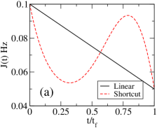
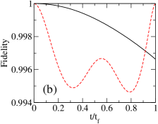
Figure 1: (a) $J(t)$ used in the shortcut protocol compared to the corresponding linear ramping. The initial and final values of $\gamma$ are $\gamma_{i}$=10, $\gamma_{f}=$20, and $t_{f}=0.08$ $t_{\rm Rabi}^{(i)}$. In panel (b) we depict the fidelity (overlap) between the evolved state and the instantaneous ground state. The number of particles and non-linearity are, $N=100$, and $U=1/(50t_{\rm Rabi}^{(i)})$ , respectively.

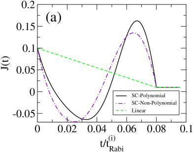
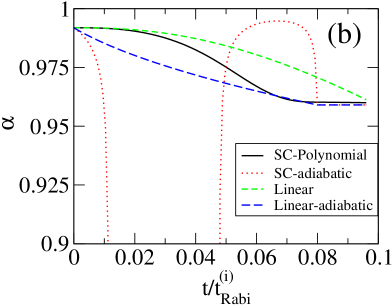
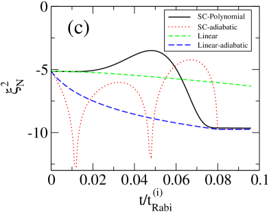
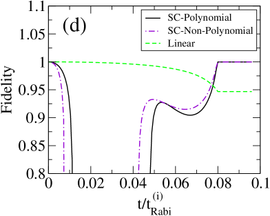
Figure 2: Panel (a): evolution of $J(t)$, (b) coherence of the state, (c) its number squeezing, and (d) the instantaneous fidelity. $N=100$ atoms, $\gamma_{i}=10$, $\gamma_{f}=100$ and $t_{f}=0.08$ $t_{\rm Rabi}^{(i)}$. For $t>t_{f}$ we fix $\gamma(t)=\gamma(t_{f})$.

For repulsive atom-atom interactions the potential in Fock space, ${\cal V}(z)$, is to a very good approximation a harmonic oscillator. Neglecting the $z$ dependence of the effective mass term and expanding $\sqrt{1-z^{2}}\simeq 1-z^{2}/2$ in ${\cal V}(z)$, the Hamiltonian in Eq. (LABEL:eq:pse) reduces to

$${\cal H}_{N}\simeq-2J\eta^{2}\partial_{z}^{2}+\frac{1}{2}(J+NU/2)z^{2},$$ (7)

A difference with respect to Ref. oursmuga and to previous applications of shortcuts-to-adiabaticity to harmonic-oscillator expansions is that now the control parameter $J(t)$ shows up both as a formal time-dependent (inverse of) mass and as an additive term in the force constant. In the Appendix  A we provide the extension of the shortcut technique for this type of time dependence when $NU/2\gg|J|$, so that we can approximate $(J+NU/2)\simeq{NU/2}$. Defining $\gamma=NU/(2J)$, this limit corresponds to $\gamma\gg 1$, which is easily attainable in current experiments. It is also relevant as it corresponds to very spin-squeezed ground states of the bosonic Josephson junction. In Appendix B we verify that the method is not applicable when $|\gamma|<1$.

For the case at hand, the inverse engineering described in Appendix A translates into solving for $J(t)$ in the following Ermakov equation,

$${\ddot{b}}-2\frac{({\dot{b}})^{2}}{b}=\frac{4k}{J(t)}b-\frac{k^{2}}{\eta^{2}}b^{5},$$ (8)

where the dots indicate time derivatives, and $k=NU/2$ and $b(t)$ must satisfy the boundary conditions

$$b_{0} \equiv b(0)=\left({8\eta^{2}J(0)\over NU}\right)^{1/4},$$ (9)

$$b_{f} \equiv b(t_{f})=\left({8\eta^{2}J(t_{f})\over NU}\right)^{1/4},$$

$$\dot{b}(0) = \ddot{b}(0)=\dot{b}(t_{f})=\ddot{b}(t_{f})=0.$$ (10)

For simplicity we apply the polynomial muga1

$$b_{\rm poly}(t) = b_{0}+10(b_{f}-b_{0})s^{3}-15(b_{f}-b_{0})s^{4}$$ (11)

$$+6(b_{f}-b_{0})s^{5}.$$

with $s=t/t_{f}$. We also consider a non-polynomial form in some comparisons,

$$b_{\rm non-poly}(t)=b_{0}\left({b_{f}\over b_{0}}\right)^{6s^{5}-15s^{4}+10s^{3}}.$$ (12)

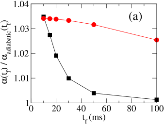
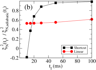
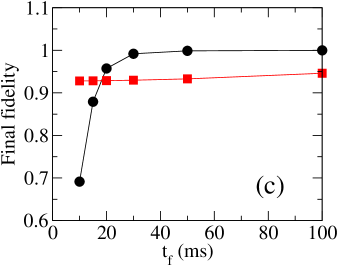
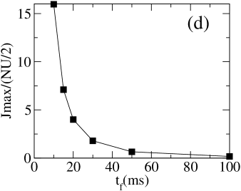
Figure 3: Properties of the state of the system at $t_{f}$ after a shortcut protocol (black) and a linear ramp (red), for different values of $t_{f}$. (a) depicts the relative coherence, $\alpha/\alpha_{\rm adiabatic}$. (b) shows the relative number squeezing, $\xi^{2}_{N}/\xi^{2}_{N,\rm adiabatic}$. (c) contains the value of the final fidelity. (d) shows the maximum value of $1/\gamma$ required for the shortcut process. In all simulations $\gamma_{i}=10$, $\gamma_{f}=100$, $N=100$, and $U=0.49$ Hz.

III Numerical simulations of the shortcut protocol

In all cases we will consider the evolution from an initial g.s. corresponding to $\gamma=\gamma_{i}$ to a final one with $\gamma=\gamma_{f}$. The control parameter $J(t)$, will go from $J(0)=J_{i}$ to $J(t_{f})=J_{f}$ in a time $t_{f}$ with a fixed value of $U$. In our first application, we will measure the time in units of the initial Rabi time, $t_{\rm Rabi}^{(i)}=\pi/J_{i}$. Later, we will consider realistic values of $U$ and $t$ taken from recent experiments.

In Fig. 1 we consider a factor 2 change in $\gamma$, from $\gamma_{i}=10$ to $\gamma_{f}=20$ in a time $t_{f}=0.08$ $t_{\rm Rabi}^{(i)}$, with $N=100$ and $NU/2=1/t_{\rm Rabi}^{(i)}$. We compare the shortcut protocol using the polynomial ansatz for $b(t)$ to a linear ramping: $J(t)=J_{i}+(J_{f}-J_{i})(t/t_{f})$. The shortcut method is shown to work almost perfectly, and we obtain a final fidelity $\simeq 1$ (despite the process being diabatic during the intermediate evolution). For this case, the linear ramping produces a final fidelity of $\simeq 0.9965$. As it occurred with the harmonic oscillator muga1 or in Ref. oursmuga , for more stringent processes, i.e. shorter final times or larger changes in $\gamma$, the method requires negative values of the control parameter. For instance, if we require a factor of 10 change, from $\gamma_{i}=10$ to $\gamma_{f}=100$ under the same conditions, $J(t)$ becomes negative during part of the evolution. Although for usual tunneling phenomena the hopping term is always positive, e.g. in external Josephson junctions, there are several proposals to implement negative or even complex hopping terms in optical lattices jz03 ; andre05 . For the internal Josephson junctions achieved in Oberthaler’s group negative tunneling presents no obstacle as they are able of engineering a tunneling term of the form (see Sect. 3.5 of Ref. ziboldphd )

$$J(t)\left[\hat{J}_{x}\ \cos\phi_{c}(t))+\hat{J_{y}}\ \sin\phi_{c}(t)\right]$$ (13)

with $\phi_{c}(t)$ a phase which can be controlled externally.

Our results are shown in Fig. 2. First we see that, for both polynomial and non-polynomial choices of $b(t)$ described above, $J$ changes its sign at intermediate times, see Fig. 2(a). This implies a transient loss of fidelity (overlap) between the evolved state and the instantaneous ground state of the system, as shown in Fig. 2(d). With the shortcut protocol both the coherence, Fig. 2(b), and number squeezing, Fig. 2(c), evolve smoothly towards their adiabatic value. In contrast, the linear ramping fails to provide the adiabatic values at the final time. The instantaneous ground state coherence, dotted red line in Fig. 2(b), is rather involved as it follows the $J(t)$ path. As seen in Fig. 2(c) the linear squeezing is $\simeq-6$ dB while the adiabatic one, accurately reproduced by the shortcut protocol, is $\simeq-10$ dB. This is a notable feature which should be experimentally accessible. The linear ramp gives a final fidelity of 0.95, well bellow those of the polynomial and non-polynomial shortcut protocols which get final fidelities of nearly 1. It is also worth stressing that the many-body state produced by the shortcut method at $t=t_{f}$ is almost an eigenstate of the system, which implies constant coherence and squeezing for $t>t_{f}$, see Fig. 2(b,c).

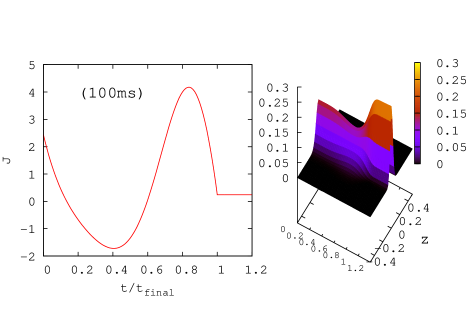
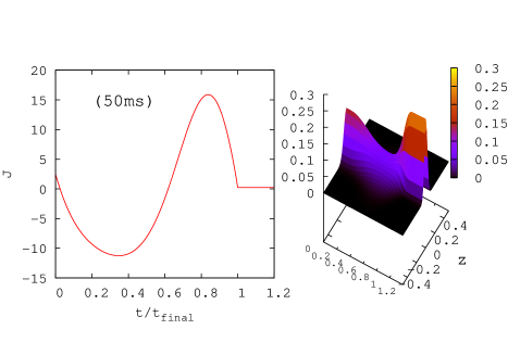
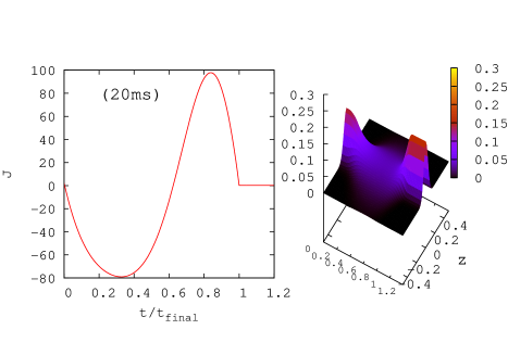
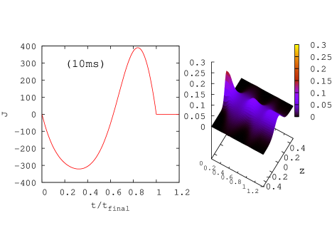
Figure 4: (left) Evolution of $J(t)$ required by the polynomial shortcut protocol for different final times $t_{f}=100,50,20,10$ ms. (right) Spectral decomposition of the many-body state $|c_{z}|^{2}$ for the same $t_{f}$ as a function of time. In all simulations $\gamma_{i}=10$, $\gamma_{f}=100$, $N=100$, and $U=0.49$ Hz.

It is also possible to engineer fidelity-one processes where the control $J(t)$ is constrained from below and above by predetermined values (in particular we could make both bounds positive). Prominent examples are the bang-bang protocols, with step-wise constant $J$, which solve the time-minimization variational problem for given bounds and boundary conditions muga2 ; muga4 ; salamon ; stef10 .

III.1 Simulations using experimental values for the parameters

As explained above, the variation of $J$ with time can be readily implemented experimentally. In this section, we will consider realistic values of the parameters. Following Refs. ziboldphd ; riedel10 we take a value of the non-linearity $U=0.49$ Hz, with $N=100$ atoms, and make variations of $\gamma$ during typical experimental values of time: $t_{f}=10,15,30,50$ and 100 ms. At $t=t_{f}$ we fix $\gamma(t)=\gamma_{f}$ and evolve the system during an additional small time to check whether the state remains close to desired final the ground state or not.

In Fig. 3 we depict the final value of the fidelity (c), number squeezing (b) and coherence of the many-body state (a), as a function of the final time imposed $t_{f}$. The shortcut method (with polynomial ansatz) is compared to the linear ramping. The first observation is that for $t_{f}>40$ ms, the shortcut protocol produces a fidelity $\simeq 1$, while the linear ramp stays always below $0.95$, see (c). Similarly, for $t_{f}>40$ ms, the final coherence and number squeezing are essentially those of the corresponding ground state (a,b). This is an important finding, as for instance the linear ramping produces roughly half of the number squeezing as compared to the adiabatic or shortcut protocol. For $t_{f}<40$ ms, the shortcut protocol is seen to fail, and in particular, the achieved final fidelities drop to $0.7$ for $t_{f}=10$ ms, smaller than the linear ramping ones. As explained above, our shortcut protocol has been derived assuming the validity of a parabolic approximation for the potential in Fock space. Therefore we expect the method to fail when the intermediate wave packet spreads far from the central region in Fock space. In Fig. 4, we have plotted the spectral decomposition of the many-body state $|c_{z}|^{2}$ as a function of time for the same final times $t_{f}$ as above. When the final time is large, the process is smooth and the wave function does not spread considerably. When we use shorter final times $J(t)$ takes large values (so $\gamma$ is small at intermediate times), and the effective wave-function spreads considerably in $z$ space. A parameter that affects the $J(t)$ functional form is the number of atoms $N$. The larger $N$, the smoother the $J(t)$ path and the better are the results obtained. This is seen in Fig. 5, where we choose only two values of $t_{f}$: $10$ and $20$ ms, and consider $N=50,100,150$ and $400$ atoms. We also depict $J(t)$, which is on average smaller for larger $N$.

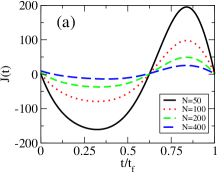
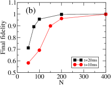
Figure 5: (a) Evolution of $J(t)$ required by the polynomial shortcut protocol for different values of $N$ and $t_{f}$=20 ms. In (b) we depict the final fidelities attained in the process for $t_{f}$=10 and $20$ ms. $U=0.49$ Hz and $\gamma_{i}=10$, $\gamma_{f}=100$.

IV Summary and conclusions

We have presented a method to produce ground states of bosonic Josephson junctions for repulsive atom-atom interactions using protocols to shortcut the adiabatic following. We inverse-engineer the accurately controllable linear coupling $J$ by mapping a Schrödinger-like equation for the (imbalance) wavefunction of the Josephson junction onto an ordinary harmonic oscillator for which shortcut protocols can be set easily. The original equation is a priori more involved for that end, as the kinetic-like term includes a time-dependent formal mass. As detailed in Appendix  A, the mapping requires a reinterpretation of kinetic and potential terms, which interchange their roles in a representation conjugate to the imbalance. The time dependence of the formal mass of the original equation (inversely proportional to $J$) implies the time dependence of the frequency of the ordinary (constant mass) harmonic oscillator, and $J$ plays finally the role of the squared frequency. This mapping is different and should be distinguished from the ones used to treat harmonic systems with a time dependent mass both in the kinetic and the potential terms l1 . From the experimental point of view, our protocol should help the production of spin-squeezed states, increasing the maximum squeezing attainable in short times. In particular, an important shortcoming of recent experimental setups ziboldphd , is that they have sizable particle loss on time scales of the order of $\simeq 50$ ms for atom numbers on the order of a few hundreds. For these systems our methods could be targeted at shorter times, as in the examples presented, providing an important improvement with respect to linear rampings.

Appendix A Shortcut equations for the Josephson junction with controllable linear coupling.

In this Appendix we shall transform the Schrödinger-like Eq. (5) so that the invariant-based engineering technique for time-dependent harmonic oscillators developed in muga1 ; muga2 may be applied. The structure of the Hamiltonian (7) is peculiar as it involves a time dependent (formal) mass factor in the kinetic-like term. The first step is to transform this Hamiltonian according to

$$\eta\to\hbar,\quad 4J(t)\to\frac{1}{m(t)},\quad\frac{NU}{2}\to k\,,$$ (14)

to rewrite Eq. (7) as

$$H=\frac{1}{2m(t)}{p}^{2}+\frac{1}{2}k{z}^{2},$$ (15)

where $p=-i\hbar\partial_{z}$ is the “momentum” conjugate to $z$ . These and other transformations performed below are formal so that the dimensions do not necessarily correspond to the ones suggested by the symbols and terminology used. For example neither $p$, $m(t)$, or $z$ have dimensions of momentum, mass and length, respectively.

Multiplying the time-dependent Schrödinger equation corresponding to Eq. (15) from the left by momentum eigenstates $\langle p|$,

$$i\hbar\partial_{t}\Psi(p,t)\! = \!-\frac{\hbar^{2}k}{2}\frac{\partial^{2}}{\partial p^{2}}\Psi(p,t)\!+\!\frac{p^{2}}{2m(t)}\Psi(p,t).$$ (16)

Finally with the new mapping

$$k \to \frac{1}{m_{x}},$$ (17)

$$\frac{1}{m(t)} \to m_{x}\omega_{x}^{2}(t),$$

$$p \to x\ ,$$

the Hamiltonian takes the standard time-dependent harmonic oscillator form

$$H=-\frac{\hbar^{2}}{2m_{x}}\frac{\partial^{2}}{\partial x^{2}}+\frac{1}{2}m_{x}\omega_{x}^{2}(t)x^{2}\ .$$ (18)

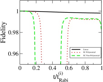
Figure 6: Instantaneous fidelity as a function of time. $\gamma_{i}=0.1$ and $\gamma_{f}=1$ with $t_{f}=t_{\rm Rabi}^{(i)}$ for the shortcut and a linear path.

Note that, thanks to the above transformations and basis change, the kinetic-like and potential-like terms in the Hamiltonian (7) have interchanged their roles so that the time dependence of the formal mass has become a time dependence of the formal frequency in Eq. (18), whereas $m_{x}$ is constant. Fast dynamics between $t=0$ and $t_{f}$, from $\omega_{x}(0)$ to $\omega_{x}(t_{f})$ without final excitations for this Hamiltonian may be inverse engineered by solving for $\omega_{x}(t)$ in the Ermakov equation muga1 ; muga2

$$\ddot{\rho}+\omega_{x}^{2}(t)\rho=\frac{\omega^{2}_{0}}{\rho^{3}}\ ,$$ (19)

where $\omega_{0}$ is in principle an arbitrary constant, and $\rho(t)$ is a scale factor for the state that we may design, e.g. with a polynomial, so that it satisfies the boundary conditions

$$\rho(0) = \left(\frac{\omega_{0}}{\omega_{x}(0)}\right)^{1/2},\;\rho(t_{f})=\left(\frac{\omega_{0}}{\omega_{x}(t_{f})}\right)^{1/2}\ ,$$

$$\dot{\rho}(0) = \dot{\rho}(t_{f})=\ddot{\rho}(0)=\ddot{\rho}(t_{f})=0.$$ (20)

Defining $b=\hbar/\rho$, choosing $\omega_{0}=k\hbar$, and undoing the changes (17) and (14) we rewrite the Ermakov equation as Eq. (8) and the boundary conditions become those in Eq. (9).

Appendix B Limitations of the method

As explained in the main text, when we have done the mapping between the results in Appendix A and the Bose-Hubbard Hamiltonian, we have assumed $NU/2\gg J$ ($\gamma\gg 1$). Thus our mapping should not be valid for small values of $\gamma$. In Fig. 6 we show that this is indeed the case. We show the predictions for the fidelity of the shortcut protocol for $\gamma_{i}=0.1$ and $\gamma_{f}=1$ for $t_{f}=t_{\rm Rabi}^{(i)}$. In this special case one finds a better fidelity with the linear ramping than with the shortcut path.

References

- (1) M. Albiez, R. Gati, J. Fölling, S. Hunsmann, M. Cristiani, and M. K. Oberthaler, Phys. Rev. Lett. 95, 010402 (2005).
- (2) J. Esteve, C. Gross, A. Weller, S. Giovanazzi, and M. K. Oberthaler, Nature 455, 1216, (2008).
- (3) C. Gross, T. Zibold, E. Nicklas, J. Estève, and M. K. Oberthaler, Nature 464, 1165 (2010).
- (4) M. F. Riedel, P. Bohi, Y. Li, T. W. Hansch, A. Sinatra, and P. Treutlein, Nature 464, 1170 (2010).
- (5) T. Zibold, E. Nicklas, C. Gross, and M. K. Oberthaler, Phys. Rev. Lett. 105, 204101 (2010).
- (6) M. Abbarchi, A. Amo, V. G. Sala, D. D. Solnyshkov, H. Flayac, L. Ferrier, I. Sagnes, E. Galopin, A. Lemaître, G. Malpuech, and J. Bloch, Nature Physics 9, 275 (2013).
- (7) T. Berrada, S. van Frank, R. Bücker, T. Schumm, J.-F. Schaff, J Schmiedmayer, Nat. Commun. 4, 2077 (2013).
- (8) R. Gati and M. K. Oberthaler, J. Phys. B.: At. Mol. Opt. Phys. 40, R61-R89 (2007).
- (9) H. J. Lipkin, N. Meshkov, and A. J. Glick, Nucl. Phys. 62, 188 (1965).
- (10) G. J. Milburn, J. Corney, E. M. Wright, and D. F. Walls, Phys. Rev. A 55, 4318 (1997).
- (11) A. J. Leggett, Rev. Mod. Phys. 73, 307 (2001).
- (12) D. J. Wineland, J. J. Bollinger, W. M. Itano, and F. L. Moore, and D. J. Heinzen, Phys. Rev. A 46, R6797 (1992).
- (13) M. Kitagawa, and M. Ueda, Phys. Rev. A 47, 5138 (1993).
- (14) B. Julia-Diaz, E. Torrontegui, J. Martorell, J. G. Muga, A. Polls, Phys. Rev. A 86, 063623 (2012).
- (15) X. Chen, A. Ruschhaupt, S. Schmidt, A. del Campo, D. Guéry-Odelin, and J. G. Muga, Phys. Rev. Lett. 104, 063002 (2010).
- (16) X. Chen, and J. G. Muga, Phys. Rev. A 82, 053403 (2010); X. Chen, E. Torrontegui, and J. G. Muga, Phys. Rev. A 83, 062116 (2011); E. Torrontegui, S. Ibañez, X. Chen, A. Ruschhaupt, D. Guéry-Odelin and J. G. Muga, Phys. Rev. A. 83, 013415 (2011).
- (17) T. Zibold, PhD thesis, U. Heidelberg (2012).
- (18) E. Nicklas, PhD thesis, U. Heidelberg (2013).
- (19) X. Chen, E. Torrontegui, D. Stefanatos, Jr-Shin Li, and J. G. Muga, Phys. Rev. A 84, 043415 (2011); E. Torrontegui, X. Chen, M. Modugno, S. Schmidt, A. Ruschhaupt and J. G. Muga, New J. Phys. 14, 013031 (2012).
- (20) A. Ruschhaupt, X. Chen, D. Alonso, and J. G. Muga, New J. Phys. 14, 093040 (2012).
- (21) X.-J. Lu, X. Chen, A. Ruschhaupt, D. Alonso, S. Guérin, and J. G. Muga, Phys. Rev. A (2013), in press (arXiv 1305.6127).
- (22) A. Sørensen, L.-M. Duan, I. Cirac, and P. Zoller, Nature 409, 603 (2001).
- (23) V. S. Shchesnovich, and M. Trippenbach, Phys. Rev. A 78, 023611, (2008).
- (24) B. Juliá-Díaz, J. Martorell, and A. Polls, Phys. Rev. A 81, 063625 (2010).
- (25) B. Juliá-Díaz, T. Zibold, M. K. Oberthaler, M. Melé-Messeguer, J. Martorell, and A. Polls, Phys. Rev. A 86, 023615 (2012).
- (26) D. Jaksch and P. Zoller, New J. Phys. 5, 56 (2003).
- (27) A. Eckardt, C. Weiss, and M. Holthaus, Phys. Rev. Lett. 95, 260404 (2005).
- (28) P. Salamon, K. H. Hoffmann, Y. Rezek, and R. Kosloff, Phys. Chem. Chem. Phys. 11, 1027 (2009).
- (29) D. Stefanatos, J. Ruths, and Jr-Shin Li, Phys. Rev. A 82, 063422 (2010).
- (30) I. A. Pedrosa, J. Math. Phys. 28 2662, (1987). C. M. A. Dantas, I. A. Pedrosa, and B. Baseia, Phys. Rev. A 45, 1320, (1992); I. A Pedrosa, G. P. Serra, and I. Guedes, Phys. Rev. A 56 4300, (1997).