The ratio method: a new tool to study one-neutron halo nuclei

Abstract

Recently a new observable to study halo nuclei was introduced, based on the ratio between breakup and elastic angular cross sections. This new observable is shown by the analysis of specific reactions to be independent of the reaction mechanism and to provide nuclear-structure information of the projectile. Here we explore the details of this ratio method, including the sensitivity to binding energy and angular momentum of the projectile. We also study the reliability of the method with breakup energy. Finally, we provide guidelines and specific examples for experimentalists who wish to apply this method.

I Introduction

One of the most intriguing phenomenon revealed by the studies with rare isotope beams is that of halo nuclei Jensen et al. (2004). Since the early experiments on reaction cross sections Tanihata et al. (1985), we have built a good understanding of the exotic features that results from the proximity to threshold and the absence of repulsive barriers Jensen and Riisager (2000). For very loosely-bound nucleons, which do not suffer the constraint of the centrifugal or Coulomb barrier, the wavefunctions develop long tails, extending well into the classically forbidden region. A primary signature of the halo phenomenon has been the sudden increase of the matter radius within a given isotopic chain Tanaka et al. (2010). In this respect, precision measurements of nuclear radii in traps open new possibilities Wang et al. (2004); Sánchez et al. (2006). Narrow momentum distributions are also an indication of the large spatial extension of the wavefunctions Zahar et al. (1993); Bazin et al. (1998). While identifying a halo can be in itself a challenge, one would also like to have a better understanding of the structure of the valence orbital and its wavefunction, such as done in $(d,p)$ studies Schmitt et al. (2012). A new observable based on a ratio of cross sections, and therefore referred to as the ratio method Capel et al. (2011), offers this possibility. In this work, we explore the ratio method in detail and provide guidelines for its application.

Over the last two decades, many nuclear halos have been discovered. Examples include the one neutron halo of ¹¹Be Fukuda et al. (2004) and the one proton halo ⁸B Smedberg et al. (1999), and both have been the focus of many studies. In the recent years, experiments have been exploring heavier halos. After the measurement of ²²C reaction cross section Tanaka et al. (2010), it was expected that ²⁶O would also exhibit a two-neutron halo structure, but now it has become clear that this halo-to-be is indeed unbound Lunderberg et al. (2012). More recently, total reaction cross section measurements on ³¹Ne have been rather inconclusive Nakamura et al. (2009) as to whether ³¹Ne is a halo. A long sequence of theoretical studies Urata et al. (2012); Sumi et al. (2012); Urata et al. (2011); Hamamoto (2010); Horiuchi et al. (2010) demonstrate that the structure information can depend strongly on the model used in the analysis of the reaction and non integrated observables may be necessary. Another possibility of a halo has been identified in the Mg chain Zhou et al. (2010) and others will surely surface with new technical developments.

As the mass increases, there are a limited number of isotopes for which $l=0,1$ orbitals are being filled in the ground state when the dripline is reached Jensen and Riisager (2000). The halo phenomenon can however be more common in these systems because it also occurs in excited states. This is certainly known to be the situation for ¹¹Be$(1/2_{1}^{-})$ and ¹⁷F$(1/2_{1}^{+})$. Interest in determining halo properties of excited states continues Ogloblin et al. (2011) but no optimum probe has been found. In principle, the new observable here discussed, can be generalized to characterize halo excited states too.

Halo nuclei are challenging from the nuclear structure point of view. Fortunately, many-body methods are now able to adequately treat the asymptotic behavior of the wavefunction of the loosely-bound nucleons Pieper (2008); Caurier and Navrátil (2006). Halo nuclei offer a unique testing ground for the understanding of the nuclear force and represent an opportunity to understand the density dependence of nuclear matter.

Due to its loosely-bound nature, the most likely method to explore halo structure is through breakup reactions. There have been important developments in the theory for the breakup of halo nuclei (see Refs. Austern et al. (1987); Yahiro et al. (1982); Sakuragi et al. (1986); Esbensen et al. (1995); Baye et al. (2005); Goldstein et al. (2006)), and today it is understood that non-perturbative non-classical approaches, which treat nuclear and Coulomb on equal footing, are needed to obtain reliable angular distributions Hussein et al. (2006); Capel et al. (2012). What is critical to understand is that the information to be extracted is model dependent, whether the process is inclusive or exclusive, whether it is nuclear or Coulomb dominated. When non-perturbative methods are used to solve the problem, the model dependence arises primarily from uncertainties in the core-target interaction Capel et al. (2004). This interaction is often poorly known, specially when the core itself is radioactive, and plays a very important role in the breakup process.

In Ref. Capel et al. (2010), Capel et al. realized that the elastic and breakup angular distributions of halo nuclei exhibit very similar features. In Ref. Capel et al. (2011) the idea of taking the ratio of these angular distributions is introduced, drawing on the Recoil Excitation and Breakup model (REB) developed earlier Johnson et al. (1997); Johnson (1999, 1998). The main advantage of this new reaction observable is that it is nearly independent of the reaction mechanism and that its sensitivity to the core-target interaction is strongly reduced. The first application presented in Ref. Capel et al. (2011) is very encouraging. Here we explore this ratio method in more detail.

This paper is organized in the following manner. In Sec. II we provide the theoretical framework. A discussion of various possible ratios is presented in Sec. III. In Sec. IV we demonstrate the validity of the ratio method and its range of validity. In Sec. V we study the structure information contained in this new observable. Finally, conclusions are drawn in Sec. VI.

II Theoretical framework

Describing the reaction of an exotic projectile $P$ impinging on a target $T$ is a complex many-body problem. While many-body techniques have made important advances to handle a number of reactions, for example capture reactions on light nuclei Navrátil et al. (2010); Navrátil and Quaglioni (2011, 2012) and nucleon elastic scattering Hagen and Michel (2012), these techniques are not able to handle the general heavy-ion reaction $P+T$ problem. In that case, it is imperative to identify the relevant degrees of freedom and address the problem within a few-body framework.

If the nucleus under study (the projectile) has a one-neutron halo, there is a strong decoupling of the core degrees of freedom from the valence neutron Jensen et al. (2004). The projectile can then be described as a two-body system: a neutron $n$ loosely bound to a core $c$, i.e. $P=c+n$. In such a scenario, one can describe the states of the system with a mean field $V_{cn}$ that reproduces basic features, such as binding energy and radius, excited states or resonances, etc. Assuming the target is well bound and focusing on elastic breakup only, the implicit inclusion of target excitation through the imaginary part of optical potentials should be sufficient. In this case, one can reduce the reaction $P+T$ to a three-body problem. This is the approach considered here. To retain simplicity in our discussion, we consider the target and the core to be structureless and of spin zero although all the formalism can be extended to include target and core spins.

II.1 The three-body model for nuclear reactions

In this model, the projectile $P=c+n$ is described by the Hamiltonian

$$H_{0}=-\frac{\hbar^{2}}{2\mu}\Delta+V_{cn}(\mbox{\boldmath$r$}),$$ (1)

where $r$ is the $c$-$n$ relative coordinate and $\mu=m_{n}m_{c}/(m_{n}+m_{c})$ is the $c$-$n$ reduced mass, with $m_{n}$ and $m_{c}$ the masses of the neutron and of the core, respectively. As mentioned above, $V_{cn}$ is a phenomenological mean field that captures some essential aspects of the halo projectile and in principle could be microscopically derived (we assume it has central and spin-orbit terms, see Appendix B for details).

The eigenstates of $H_{0}$ are solutions of

$$H_{0}\phi_{ljm}(E,\mbox{\boldmath$r$})=E\phi_{ljm}(E,\mbox{\boldmath$r$}),$$ (2)

where $E$ is the $c$-$n$ relative energy. The total angular momentum $j$ results from the coupling of the orbital angular momentum $l$ and the spin of the valence neutron; $m$ is its projection. Negative-energy states correspond to $c$-$n$ bound states. They are normalized to unity. We denote by $\{\phi_{l_{i}j_{i}m_{i}}\}_{i=0,1,\ldots}$ these bound states of energy $E_{i}<0$, with $i=0$ corresponding to the projectile ground state, $i=1$ to its first excited (bound) state, etc. Positive-energy states describe the $c$-$n$ continuum. Their radial part is normalized according to

$$u_{lj}(E,r)\mathop{\longrightarrow}\limits_{{r}\rightarrow{\infty}}\sqrt{\frac{2\mu}{\pi\hbar^{2}k}}\left[\cos\delta_{lj}F_{l}(kr)+\sin\delta_{lj}G_{l}(kr)\right],$$ (3)

where $k=\sqrt{2\mu E/\hbar^{2}}$ is the wave number, $\delta_{lj}$ is the nuclear phase shift at energy $E$, and $F_{l}$ and $G_{l}$ are regular and irregular Coulomb functions, respectively Abramowitz and Stegun (1970), taken for zero Sommerfeld parameter. This normalization has been chosen so that

$$\langle\phi_{ljm}(E)|\phi_{ljm}(E^{\prime})\rangle=\delta(E-E^{\prime}).$$ (4)

With this two-body description for the projectile, the $P$-$T$ collision reduces to a three-body problem whose Hamiltonian reads

$$H_{\rm 3b}(\mbox{\boldmath$R$},\mbox{\boldmath$r$})=\hat{T}_{\mbox{\boldmath$R$}}+H_{0}(\mbox{\boldmath$r$})+U_{cT}(\mbox{\boldmath$R$}_{c})+U_{{\rm n}T}(\mbox{\boldmath$R$}_{n}),$$ (5)

where $R$ is the coordinate of the projectile center of mass relative to the target. In Eq. (5), additional optical potentials have been introduced to describe the scattering of the core off the target $U_{cT}$ and the neutron off the target $U_{nT}$. These optical potentials are typically phenomenological and contain an important imaginary term to account for other reaction channels not explicitly included in this description. Since they are not uniquely defined, these potentials may induce significant uncertainties in the analysis of the reactions modeled within this framework Capel et al. (2004).

In order to study the reactions of $P$ on $T$ we need to solve the three-body Schrödinger equation

$$H_{\rm 3b}\Psi(\mbox{\boldmath$R$},\mbox{\boldmath$r$})=E_{\rm tot}\Psi(\mbox{\boldmath$R$},\mbox{\boldmath$r$}).$$ (6)

As customary, we align the initial momentum $\mbox{\boldmath$K$}_{0}$ with the $Z$ axis and assume the projectile to be initially in its ground state, so that:

$$\Psi(\mbox{\boldmath$R$},\mbox{\boldmath$r$})\mathop{\longrightarrow}\limits_{{Z}\rightarrow{-\infty}}e^{iK_{0}Z}\phi_{l_{0}j_{0}m_{0}}(\mbox{\boldmath$r$}).$$ (7)

The total energy of the system is then given by $E_{\rm tot}=\hbar^{2}K_{0}^{2}/2\mu_{PT}+E_{0}$, where $\mu_{PT}$ is the $P$-$T$ reduced mass.

II.2 The Dynamical Eikonal Approximation

It is important to identify a method for solving the three-body problem (6), that reliably describes elastic and breakup of loosely-bound nuclei. While the momentum-space integral Faddeev method Deltuva (2009a, b) is considered exact, its present implementation is limited to $d+T$ reactions where the target charge is $Z_{T}\leq 20$. The Continuum Discretized Coupled Channel (CDCC) method Austern et al. (1987); Yahiro et al. (1982); Sakuragi et al. (1986) compares well with the Faddeev method Upadhyay et al. (2012), however it is still computationally intensive. A detailed comparison of the Dynamical Eikonal Approximation (DEA) Baye et al. (2005); Goldstein et al. (2006) with CDCC shows that DEA is a very good approximation to the problem for beam energies $E\geq 40$ MeV/nucleon Capel et al. (2012). Because this method is less computationally intensive, DEA is used in LABEL:ratio-plb and here to demonstrate the ratio method.

A well known and useful approach to reactions at high energies is the eikonal approximation Glauber (1959); Baye et al. (2005); Goldstein et al. (2006). Motivated by the boundary form (7), the three-body wave function $\Psi(\mbox{\boldmath$R$},\mbox{\boldmath$r$})$ is factorized as

$$\Psi^{\rm DEA}(\mbox{\boldmath$R$},\mbox{\boldmath$r$})=e^{iK_{0}Z}\widehat{\Psi}(\mbox{\boldmath$R$},\mbox{\boldmath$r$}).$$ (8)

At high energies, one expects a weak dependence on $R$ of $\widehat{\Psi}$. Using the factorization (8) in Eq. (6) and neglecting second-order derivatives of $\widehat{\Psi}$ with respect to $R$, we obtain Goldstein et al. (2006)

$$i\frac{\hbar^{2}K_{0}}{\mu_{PT}}\frac{\partial}{\partial Z}\widehat{\Psi}(Z,\mbox{\boldmath$b$},\mbox{\boldmath$r$})$$ (9)

$$= \left[(H_{0}-E_{0})+U_{cT}(\mbox{\boldmath$R$}_{c})+U_{nT}(\mbox{\boldmath$R$}_{n})\right]\widehat{\Psi}(Z,\mbox{\boldmath$b$},\mbox{\boldmath$r$}),$$

where $Z$ and $b$ are the longitudinal and transverse components of $R$, respectively. In the standard eikonal implementation, a subsequent adiabatic approximation is performed to solve Eq. (9). That approximation corresponds to neglect the excitation energy of the projectile compared to the beam energy. In DEA, no such an adiabatic approximation is made and Eq. (9) is solved numerically for each $b$ imposing the condition: $\widehat{\Psi}(Z\rightarrow-\infty,\mbox{\boldmath$b$},\mbox{\boldmath$r$})=\phi_{l_{0}j_{0}m_{0}}(\mbox{\boldmath$r$})$, in agreement with condition (7). The S-matrix is then extracted from the asymptotic behavior $\widehat{\Psi}(Z\rightarrow+\infty,\mbox{\boldmath$b$},\mbox{\boldmath$r$})$ as detailed in LABEL:dea2. Note that since this does not imply any semiclassical hypothesis, DEA is a fully quantal model Goldstein et al. (2006); Capel et al. (2012).

II.3 The recoil excitation and breakup model

In the nineties, Johnson et al. realized that a simple factorization of the scattering amplitude can be obtained when a neutron halo projectile interacts with the target Johnson et al. (1997). The key ingredients to the so-called Recoil Excitation and Breakup (REB) model are i) neglecting the valence particle’s interaction with the target, and ii) assuming the excitation energy of the projectile is small compared to the beam energy (the adiabatic approximation). When these two conditions are satisfied, the elastic-scattering cross sections becomes Johnson et al. (1997); Johnson (1999):

$$\left(\frac{d\sigma}{d\Omega}\right)_{\rm el}=|F_{0,0}(\mbox{\boldmath$Q$})|^{2}\;\left(\frac{d\sigma}{d\Omega}\right)_{\rm pt}$$ (10)

where $|F_{0,0}(\mbox{\boldmath$Q$})|^{2}$ is a form factor accounting for the extension of the halo [see Eq. (11) below], and $\left(\frac{d\sigma}{d\Omega}\right)_{\rm pt}$ is a cross section for a point-like projectile with mass $\mu_{PT}$, scattered by the core-target interaction $U_{cT}$. The relation (10) is often mistaken for the first-order perturbation theory although it does not involve the Born approximation. Note that $\left(\frac{d\sigma}{d\Omega}\right)_{\rm pt}$ is similar to the experimental core-target elastic scattering, but for a different projectile mass.

The form factor is defined by:

$$|F_{0,0}(\mbox{\boldmath$Q$})|^{2}=\frac{1}{2j_{0}+1}\sum_{m_{0}}\left|\int|\phi_{l_{0}j_{0}m_{0}}(\mbox{\boldmath$r$})|^{2}e^{i\mbox{\boldmath$Q\cdot r$}}d\mbox{\boldmath$r$}\right|^{2},$$ (11)

and represents the Fourier transform of the halo ground state density. Here $\mbox{\boldmath$Q$}=\frac{m_{n}}{m_{c}+m_{n}}(K_{0}\mbox{\boldmath$\widehat{Z}$}-\mbox{\boldmath$K$}^{\prime})$ is proportional to the momentum transferred during the scattering process. It modulates the diffraction pattern contained in the point-like cross section, determining which are the relevant scattering angles to be considered in the process

$$Q=2\frac{m_{n}}{m_{c}+m_{n}}K_{0}\sin(\theta/2).$$ (12)

In LABEL:capel10, it was realized that the elastic and breakup cross sections have similar diffraction patterns, a fact only fully understood with the subsequent work on the ratio method Capel et al. (2011). In LABEL:ratio-plb, we used the fact that the factorization (10) can be generalized to angular distributions for the excitation of the projectile to any of its state, either bound or not Johnson (1999, 1998). For inelastic scattering with excitation to bound state $i>0$, we can define the form factor

$$|F_{i,0}(\mbox{\boldmath$Q$})|^{2}$$ (13)

$$= \frac{1}{2j_{0}+1}\sum_{m_{0}}\sum_{m_{i}}\left|\int\phi_{l_{i}j_{i}m_{i}}(\mbox{\boldmath$r$})\phi_{l_{0}j_{0}m_{0}}(\mbox{\boldmath$r$})e^{i\mbox{\boldmath$Q\cdot r$}}d\mbox{\boldmath$r$}\right|^{2},$$

while for breakup to energy $E$, we use the form factor

$$|F_{E,0}(\mbox{\boldmath$Q$})|^{2}$$ (14)

$$= \frac{1}{2j_{0}+1}\sum_{m_{0}}\sum_{ljm}\left|\int\phi_{ljm}(E,\mbox{\boldmath$r$})\phi_{l_{0}j_{0}m_{0}}(\mbox{\boldmath$r$})e^{i\mbox{\boldmath$Q\cdot r$}}d\mbox{\boldmath$r$}\right|^{2},$$

where $\phi_{ljm}(E,\mbox{\boldmath$r$})$ is the eigenstate of $H_{0}$ at positive energy $E$ in the partial wave $ljm$ [see Eq. (2)]. The REB prediction for the inelastic cross section, i.e. the angular distribution for the projectile excited to state $i$ while scattered in direction $\Omega$ reads

$$\left(\frac{d\sigma_{i}}{d\Omega}\right)_{\rm inel}=|F_{i,0}(\mbox{\boldmath$Q$})|^{2}\;\left(\frac{d\sigma}{d\Omega}\right)_{\rm pt}.$$ (15)

Similarly, we get the following angular distribution for breakup, i.e. the cross section for the projectile being broken up at an energy $E$ in the $c$-$n$ continuum with its center of mass scattered in direction $\Omega$

$$\left(\frac{d\sigma}{dEd\Omega}\right)_{\rm bu}=|F_{E,0}(\mbox{\boldmath$Q$})|^{2}\;\left(\frac{d\sigma}{d\Omega}\right)_{\rm pt}.$$ (16)

Neglecting the small difference in magnitude between the outgoing momenta for elastic and inelastic processes, the point-like cross section $\left(d\sigma/d\Omega\right)_{\rm pt}$ is identical for all three processes (10), (15), and (16). This first explains the result obtained in LABEL:capel10, where it was observed that the angular distributions for elastic scattering and breakup exhibit very similar patterns. Indeed, most of the angular dependence of these cross sections is due to that point-like cross section. Second, the similarity of the expressions (10), (15), and (16) is at the core of the ratio method. If we now consider the ratio between Eqs. (16) and (10), the point-like cross sections cancel out, leaving an observable which, within the REB model, is just the ratio of form factors

$${\cal R}_{\rm el}(E,\mbox{\boldmath$Q$}) = \frac{(d\sigma/dEd\Omega)_{\rm bu}}{(d\sigma/d\Omega)_{\rm el}}$$ (17)

$$\stackrel{{\scriptstyle\rm(REB)}}{{=}} \frac{|F_{E,0}(\mbox{\boldmath$Q$})|^{2}}{|F_{0,0}(\mbox{\boldmath$Q$})|^{2}}.$$ (18)

Therefore, according to the REB predictions, this ratio should be sensitive only to the structure of the projectile and be independent of the reaction mechanism. In particular, considering the ratio (17) automatically removes the dependence on the core-target interaction, which is the most ambiguous input in reaction modeling.

III Ratios of cross sections

Before analyzing the structure content of this new observable, we should point out that identical cancellations of the point-like cross section can be obtained for the ratio of any linear combination of breakup, elastic- and inelastic-scattering angular distributions. Therefore we consider here, in addition to ${\cal R}_{\rm el}$ (17), other options. Because in some halo systems, there is a nearby excited state, hard to disentangle from the ground state, the elastic and inelastic contributions may be easier to measure together. We then introduce the quasi-elastic ratio

$${\cal R}_{\rm quasi}(E,\mbox{\boldmath$Q$}) = \frac{(d\sigma/dEd\Omega)_{\rm bu}}{(d\sigma/d\Omega)_{\rm quasi}}$$ (19)

$$\stackrel{{\scriptstyle\rm(REB)}}{{=}} \frac{|F_{E,0}(\mbox{\boldmath$Q$})|^{2}}{|F_{0,0}(\mbox{\boldmath$Q$})|^{2}+\sum_{i>0}|F_{i,0}(\mbox{\boldmath$Q$})|^{2}},$$ (20)

where $(d\sigma/d\Omega)_{\rm quasi}=(d\sigma/d\Omega)_{\rm el}+\sum_{i>0}(d\sigma_{i}/d\Omega)_{\rm inel}$. Because for low $Q$, elastic scattering is dominant, adding the breakup does not make much difference to the ratio observables but simplifies the form factor dependence. Thus, we also consider

$${\cal R}_{\rm sum}(E,\mbox{\boldmath$Q$}) = \frac{(d\sigma/dEd\Omega)_{\rm bu}}{(d\sigma/d\Omega)_{\rm sum}}$$ (21)

$$\stackrel{{\scriptstyle\rm(REB)}}{{=}} |F_{E,0}(\mbox{\boldmath$Q$})|^{2},$$ (22)

where the summed cross section reads

$$\left(\frac{d\sigma}{d\Omega}\right)_{\rm sum}$$ (23)

$$= \left(\frac{d\sigma}{d\Omega}\right)_{\rm el}+\sum_{i>0}\left(\frac{d\sigma_{i}}{d\Omega}\right)_{\rm inel}+\int\left(\frac{d\sigma}{dEd\Omega}\right)_{\rm bu}dE.$$

Figure 1: Ratios (18), (20) and (22) suggested by the similarity between angular distributions for elastic scattering and breakup. The calculations are performed within REB for ¹¹Be impinging on Pb at 69 MeV/nucleon considering a ¹⁰Be-$n$ continuum energy $E=0.1$ MeV.

We compare in Fig. 1 the REB prediction for ${\cal R}_{\rm el}$ (18), ${\cal R}_{\rm quasi}$ (20) and ${\cal R}_{\rm sum}$ (22) for the reaction of ¹¹Be on ²⁰⁸Pb at 69 MeV/nucleon. The transferred momentum $Q$ has been converted into the center-of-mass scattering angle following Eq. (12). As expected there is very little difference between ${\cal R}_{\rm el}$ and ${\cal R}_{\rm quasi}$. Adding the breakup angular distribution to the denominator modifies only the large-angle behavior of the ratio. Other possibilities for the ratio are discussed in Appendix A.

After close analysis and a number of exploratory calculations, we found it optimal to consider the ratio ${\cal R}_{\rm sum}$. This ratio leads to the simplest REB prediction (22) and is probably the easiest to measure experimentally. In LABEL:ratio-plb we quantified this ratio with DEA calculations that do not make the approximations of the REB model, and presented the argument that the REB approximations can be justified in realistic cases. Here we focus the discussion on the source of the small discrepancies found between DEA calculations and REB predictions and the structure information that can be extracted from ${\cal R}_{\rm sum}$.

IV Analysis of the cross section ratio

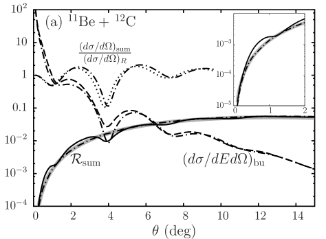
Figure 2: Illustration of the ratio method for ¹¹Be impinging on: (a) C at 67 MeV/nucleon, and (b) Pb at 69 MeV/nucleon. Summed cross sections (dotted lines) and breakup angular distributions (dashed lines) computed within DEA are compared to their ratio ${\cal R}_{\rm sum}$ (thin solid lines), which is found in excellent agreement with its REB prediction $|F_{E,0}|^{2}$ (thick grey line). Calculations with $U_{nT}=0$ are shown as dash-dotted lines. The insets focus on the forward-angle behavior of the ratio.

For the purpose of illustration, we base our calculations on a concrete reaction measured at RIKEN Fukuda et al. (2004), namely the breakup of ¹¹Be on C and Pb at 67 and 69 MeV/nucleon, respectively. In our two-body description of the projectile, ¹¹Be is seen as an inert ¹⁰Be core in its $0^{+}$ ground state, to which a neutron is bound by $E_{0}=-0.5$ MeV in the $1s_{1/2}$ orbit. Unless mentioned otherwise, we take the same inputs as in LABEL:ratio-plb (all interactions are provided in our Appendix B) and perform calculations within DEA, which is found in excellent agreement with these experimental data Goldstein et al. (2006).

In Fig. 2 we show the corresponding summed cross sections (23) as a ratio to Rutherford (dotted lines), the angular distributions for breakup at a continuum energy $E=0.1~{}{\rm MeV}$ in units b/MeV (dashed lines), as well as their ratios ${\cal R}_{\rm sum}$ (21) in units MeV^-1 (solid lines). The continuum energy $E=0.1$ MeV is at this point arbitrary. We will discuss it in detail in Sec. V.4. If all works well, that ratio ${\cal R}_{\rm sum}$ should agree with $|F_{E,0}|^{2}$ Eq. (14), as predicted by the REB model (22) (thick grey line). And, indeed, we find the agreement to be very good. In both cases, most of the angular dependence of the cross sections has been removed by taking their ratio, leaving a curve varying smoothly with the scattering angle $\theta$. Moreover, this ratio lies nearly on top of its REB prediction. As already pointed out in LABEL:ratio-plb, this implies that the ratio ${\cal R}_{\rm sum}$ removes most of the dependence on the reaction mechanism and hence contains mostly structure information. We note the presence of residual oscillations at forward angles for the C target and at larger angles for the Pb target. Note also the slower rise at the most forward angles in the latter case (see the insets, which focus on the forward-angle region). In the next subsections we explore the source for these small discrepancies.

IV.1 The REB cross sections

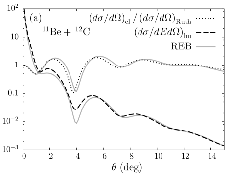
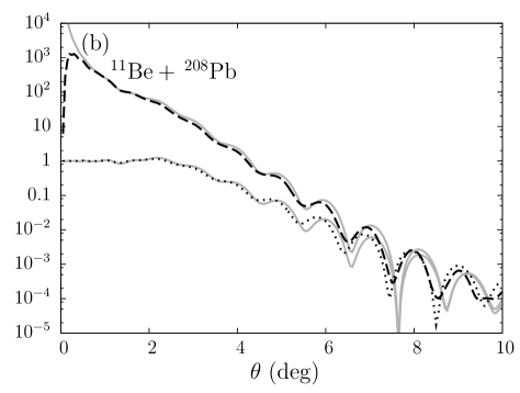
Figure 3: Comparison of REB and DEA predictions for the elastic and breakup angular distributions for ¹¹Be: (a) on ¹²C at 67 MeV/nucleon and (b) on ²⁰⁸Pb at 69 MeV/nucleon. The dotted(dashed) line corresponds to the elastic(breakup) scattering within DEA and the grey lines to results with REB.

The validity of the ratio (17) depends crucially on the equality of the two point-like cross sections in Eqs. (10) and (16). So here we test explicitly the validity of these equations. In Fig. 3 we compare the results of Eqs. (10) and (16) with those obtained in the full dynamical calculation (DEA), for our two examples, namely ¹¹Be on ¹²C (a) and ¹¹Be on ²⁰⁸Pb (b). The dotted and dashed lines correspond to the DEA angular distributions for the elastic and breakup cross sections, respectively. The grey lines are obtained with the factorization in Eqs. (10) and (16). For the light target, the REB follows closely the DEA result in both elastic and breakup processes but for a slight shift in the oscillatory pattern. The same can be seen for the Pb target with the exception of smaller angles. In this regime, the breakup cross section is not well described by REB. In the next two subsections we will discuss the two approximations present in the REB model and their imprint on the discrepancies seen in Fig. 3.

IV.2 Role of $U_{nT}$

The REB model neglects the contribution of $U_{nT}$ and this explains why the form factor $|F_{E,0}|^{2}$ is perfectly smooth, whereas the DEA ratio exhibits residual oscillations. The neutron interaction with the target gives the projectile a minor kick that causes a slight shift in the diffractive pattern, as already noted by Johnson et al. Johnson et al. (1997) and confirmed in Fig. 3. A careful analysis of the angular distributions shows that this shift depends slightly on the excitation energy of the projectile. The oscillatory pattern in the dynamical calculations therefore differs between elastic, inelastic, and breakup cross sections, leading to the residual oscillations in their ratio. To confirm this analysis, we repeat the DEA calculations setting $U_{nT}=0$ (dash-dotted lines in Fig. 2). The angular distributions obtained in this manner are exactly in phase and their ratios exhibit no residual oscillations. These ratios are in perfect agreement with the REB predictions but for the very forward-angle region on the Pb target (see inset of Fig. 2(b)). In that region, setting $U_{nT}=0$ does not improve the agreement between DEA and REB. The reason for that difference has to be looked for in the second ingredient of the REB model, i. e. the adiabatic approximation (see Sec. IV.3).

Even though $U_{nT}$ has an effect on the dynamics, when applying the ratio method to data it is likely that the residual oscillations will not be noticeable experimentally with current angular resolutions. In Fig. 4 we show the ratio obtained with DEA (solid line), that predicted by the REB model (thick grey line) and that obtained after folding the DEA angular distributions with a typical experimental resolution (dash-dotted line). To this end, we convolute the theoretical cross sections with a Gaussian of standard deviation $0.41^{\circ}$, which corresponds to the angular resolution of the RIKEN experiment Fukuda et al. (2004). In Fig. 4(a) we show the log plot, and to emphasize the difference we include Fig. 4(b) with the corresponding linear plot. As expected the convolution reduces the residual oscillations to the point where they would no longer be detectable.

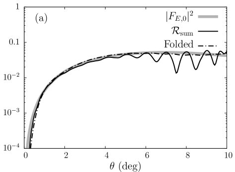
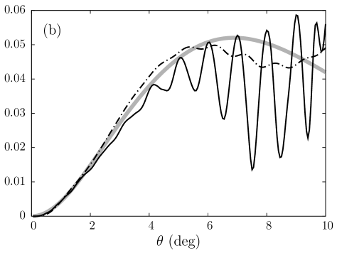
Figure 4: Smoothing of the angular distributions by the folding with experimental angular resolution (¹¹Be on Pb at 69 MeV/nucleon): (a) log plot; (b) linear plot.

IV.3 Role of the adiabatic approximation

In addition to neglecting $U_{nT}$, the REB model neglects the excitation energy of the projectile (adiabatic approximation). This second approximation is responsible for the different slope of the ratio ${\cal R}_{\rm sum}$ and its REB prediction at the most forward angles on the Pb target (see inset of Fig. 2(b)).

The Fig. 3(b) shows very clearly that at very forward angles, the elastic scattering is well described by REB but the breakup cross section is not, introducing an unphysical divergence. One could arrive at these same conclusions directly by analysing the $Q$-dependence of Eqs. (10) and (16). It is for this reason that the REB ratio (22) is higher than the correct ${\cal R}_{\rm sum}$ at forward angles, as shown in the inset of Fig. 2(b). The adiabatic—or sudden—approximation assumes a very brief interaction time with the target. When the reaction is entirely dominated by the Coulomb interaction, which is the case for breakup on Pb at forward angles, it cannot be treated satisfactorily within the adiabatic approximation due to the infinite range of the Coulomb potential. Note that the overestimation of the ratio by the REB is not observed for the carbon target. In that case the reaction is dominated by short-ranged nuclear interactions, which allow us to rely on the adiabatic approximation Goldstein et al. (2006).

This analysis shows that the effects of the adiabatic approximation upon the ratio are small and limited to the very forward angles for Coulomb-dominated reactions. Since cross sections in this region can hardly be measured, it is very unlikely that these effects will ever be noticeable. Nevertheless this analysis will help us understand differences between DEA calculations and REB predictions observed in later subsections.

IV.4 Independence of the ratio on the reaction process

In LABEL:ratio-plb we showed that the ratio obtained when considering the C target is identical to that obtained with a Pb target. In other words, the new observable is independent of the reaction mechanism. To appreciate this fact we emphasize the difference between the breakup and summed distributions obtained on C and on Pb (compare dotted and dashed lines in Fig. 2(a) and (b)). Even though the cross sections are orders of magnitude apart, and their diffraction pattern is completely different, still the resulting ratio is very close to the form factor Eq. (14) as predicted by REB.

In Fig. 5 we focus on the reaction on Pb and explore the interplay between Coulomb and nuclear interactions. In addition to DEA calculations including Coulomb and nuclear interactions (C.+N., solid line), we show results obtained from DEA calculations where only the Coulomb term of the $U_{cT}$ optical potential is considered (Coul., dashed line). As already observed in LABEL:capel10, the angular distributions vary strongly with the $P$-$T$ potential, indicating the sensitivity of the reaction mechanism to that potential choice. Nevertheless, both ratios fall on top of the form factor, confirming the independence of the ratio to the reaction process. The residual oscillations are significantly reduced when only the Coulomb interaction is present. This is due to a much smoother behavior of the angular distributions when no nuclear interaction is included Capel et al. (2010).

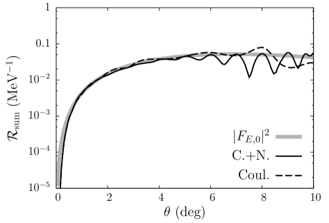
Figure 5: Ratio computed for ¹¹Be on Pb at 69 MeV/nucleon using different interactions: Coulomb plus nuclear (solid line) and purely Coulomb (dashed line) $P$-$T$ potentials.

To complete this analysis of the sensitivity of the ratio to the reaction mechanism, we now turn to its variation with the beam energy. In Fig. 6, $\cal{R}_{\rm sum}$ is plotted for ¹¹Be impinging on Pb at 40, 69, and 100 MeV/nucleon. As detailed in Appendix B, the optical potentials $U_{cT}$ and $U_{nT}$ are adapted to the beam energy, while the projectile description is kept unchanged. To compare all three ratios to one another, they are plotted as a function of $Q$ Eq. (12). The most significant difference between all three calculations are observed at large $Q$, where the ratios exhibit residual oscillations. As explained in Sec. IV.2, they are due to $U_{nT}$, which varies with the beam energy. Another, though smaller, difference is observed at very small $Q$, corresponding to very forward angle (see inset of Fig. 6). In that region, the DEA underestimates its REB prediction because of the adiabatic approximation (see Sec. IV.3). Since the REB approximation is more reliable at high beam energy, the agreement between DEA and REB improves at forward angles when larger energies are considered.

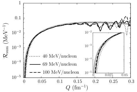
Figure 6: Ratio computed on Pb at different beam energies.

IV.5 Applicability to other one-neutron halo systems

To check the applicability of the ratio method to other halo nuclei, we study the case of ¹⁹C. This one-neutron halo nucleus has been studied experimentally by various groups. We choose here the conditions of the RIKEN experiment, i. e. performed at 67 MeV/nucleon on a lead target nakamura99 . In Fig. 7, the DEA summed (dotted line) and breakup (dashed line) cross sections are plotted as a function of the scattering angle $\theta$ of the ¹⁸C-$n$ center of mass together with the corresponding ratio ${\cal R}_{\rm sum}$ (solid line) and its REB prediction (thick gray line). Here we assumed the final breakup state to be a non-resonant state at $E=0.3$ MeV. The results in Fig. 7 are very similar to those observed in Fig. 2(b) for ¹¹Be: both angular distributions exhibit similar features that are mostly removed when taking their ratio. This confirms the validity of the ratio method for other one-neutron halo projectiles.

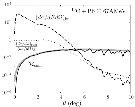
Figure 7: Analysis of the ratio for ¹⁹C on Pb at 67 MeV/nucleon: summed cross section (dotted), breakup cross section (dashed) and ratio (solid) versus the REB prediction (thick grey).

V Structure information contained in the cross section ratio

Now that we have a good understanding of the small discrepancies of the true ratio and the prediction from the REB model, we can explore the structure information contained in this observable. Having shown the ratio to be independent of the reaction process, we expect it to be more sensitive to the projectile structure than usual reaction observables. Below we discuss the dependence on the binding energy of the halo neutron $E_{0}$, its orbital angular momentum $l_{0}$, the details of the $c$-$n$ radial wavefunction, and the final scattering state. For this analysis, we stick to the collision of ¹¹Be on Pb at 69/nucleon.

V.1 Binding energy

The ratio ${\cal R}_{\rm sum}$ is very sensitive to the one-neutron separation energy $E_{0}$. Because the breakup cross section is larger for loosely bound systems, the magnitude of the ratio increases with decreasing binding Capel et al. (2011). In Fig. 8, we show the ratio obtained for a ¹¹Be-like system bound by 50 keV, 0.5 MeV, and 5.0 MeV, respectively. They result from DEA calculations where the depth of the ¹⁰Be-$n$ interaction in the $s$ wave is adjusted to reproduce the appropriate one-neutron separation energy (see Appendix B). Our results show that changing the binding energy by one order of magnitude produces a change in the ratio by two orders of magnitude. Moreover, the shape of the ratio differs significantly from one binding energy to the other. Looking into the details of the angular distributions one sees also that the agreement with the REB prediction deteriorates with increasing binding energy. This is to be expected since for large binding energy, the excitation energy needed for breakup is large and the adiabatic approximation is no longer justified. Nevertheless, it is clear that the cross section ratio provides a very accurate indirect measurement of the binding energy of the system.

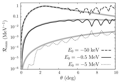
Figure 8: Sensitivity of ratio ${\cal R}_{\rm sum}$ to the binding energy of the projectile: $E_{0}=-50$ keV, $-0.5$ MeV, and $-5$ MeV.

V.2 Orbital angular momentum

Next we investigate the dependence on the orbital angular momentum of the initial bound state $l_{0}$. The ¹⁰Be-$n$ interaction is adjusted to reproduce a ¹¹Be ground state at $E_{0}=-0.5$ MeV with, instead of the $1s_{1/2}$ configuration, a $0p_{1/2}$ and a $0d_{5/2}$ configuration (see Appendix B). DEA calculations are repeated with these new interactions, and the resulting ratios are plotted in Fig. 9. Again we find that the cross section ratio is very sensitive to this property of the projectile initial state. The magnitude of the ratio decreases with increasing angular momentum. It is important to note that even though the magnitude for a 5 MeV bound $1s_{1/2}$ state (Fig. 8) is similar to that of a $0.5$ MeV $0d_{5/2}$ state (Fig. 9), the shape of the distribution is very different, particularly the slope at larger angles. This feature would make it possible to determine unequivocally both the binding energy and the angular momentum of the nucleus under inspection.

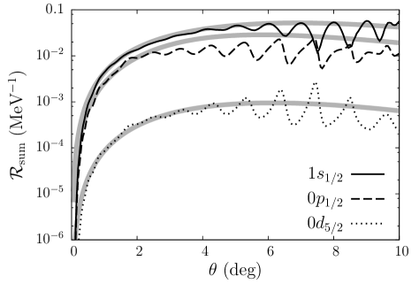
Figure 9: Sensitivity of ratio ${\cal R}_{\rm sum}$ to the orbital angular momentum of the halo neutron. Calculations with a valence neutron bound to a ¹⁰Be core by $E_{0}=-0.5$ MeV in a $1s_{1/2}$, $0p_{1/2}$ or $0d_{5/2}$ orbital are compared to one another.

V.3 Radial wave function

We now turn to the sensitivity of the ratio to details of the projectile radial wavefunction. We consider various geometries for $V_{cn}$ in the $s$ wave and readjust the depth of the interaction to reproduce the physical neutron separation energy $E_{0}=-0.5$ MeV (see Appendix B). Namely we vary the radius and the number of nodes of the initial state. The resulting radial wavefunctions are presented in Fig. 10(a). We repeat DEA calculations for the reaction on Pb at 69 MeV/nucleon. The corresponding ratios ${\cal R}_{\rm sum}$ folded with experimental resolution and their REB predictions are plotted in Fig. 10(b). At forward angles, i.e. in the range $1^{\circ}$ to $3^{\circ}$, the DEA ratios are in excellent agreement with their REB predictions. In that region, the ratio is proportional to the square of the asymptotic normalization coefficient (ANC). At larger angles, the discrepancy between DEA and REB increases. Nevertheless, the general behavior, and especially the ordering of the curves, is the same in both models. In particular, the REB predicts a crossing of the curves, that actually takes place at $\theta\simeq 6^{\circ}$ in dynamical calculations. At that angle, the ratio obtained with the initial $0s_{1/2}$ state overtakes the others although it corresponds to the smallest ANC. This can only be explained if the ratio is sensitive to the internal part of the wave function at larger angles. The ratio is thus able to probe different parts of the radial wave function, depending on the scattering angle $\theta$. It is one of the few reaction observables to display such a property. Elastic-scattering and breakup cross sections are indeed purely peripheral, in the sense that they probe only the tail of the projectile wave function and not its interior Capel and Nunes (2006). Although these details do not affect the ratio as significantly as the binding energy and the angular momentum, we expect them to be observable in data with enough statistics.

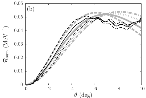
Figure 10: Sensitivity of ratio ${\cal R}_{\rm sum}$ to the radial wave function of the projectile: (a) radial wave functions of the initial $s_{1/2}$ states; (b) corresponding DEA ratios ${\cal R}_{\rm sum}$ folded with experimental resolution (thin black lines) and their REB predictions (thick gray lines).

V.4 Choice of continuum energy $E$

So far we have fixed the ¹⁰Be-$n$ relative energy in the final state to be $E=0.1$ MeV. However ${\cal R}_{\rm sum}$ can be defined for any relative energy $E$ between the core and the halo neutron after breakup. We now study the effect of this energy by considering $E=0.5$, 1.0, and 1.5 MeV. In addition, we also consider the ¹⁰Be-$n$ energy $E_{\rm res}=1.274$ MeV, which corresponds to a $5/2^{+}$ resonance in the ¹¹Be continuum. In our model, that resonance is simulated by a $d5/2$ state Capel et al. (2004). The resulting ratios are shown in Fig. 11 for a C target at 67 MeV/nucleon (a) and for a Pb target at 69 MeV/nucleon (b). For readability, the ratios have been multiplied by powers of 10: 10 for $E=0.5$ MeV, $10^{2}$ for $E=1.0$ MeV, $10^{3}$ for $E_{\rm res}$, and $10^{5}$ for $E=1.5$ MeV. As expected from the above analysis, the agreement between DEA calculations (solid lines) and REB predictions (thick gray lines) worsens with increasing continuum energy $E$. On both targets, the residual oscillations increase at larger $E$. This effect is caused by the shift due to $U_{nT}$, which increases with $E$ (see Sec. IV.2). The difference in the oscillatory pattern between the elastic scattering and the breakup angular distributions therefore increases at larger $E$, leading to more significant residual oscillations in the ratio. This disagreement between DEA calculations and the REB predictions fully disappears when $U_{nT}$ is set to 0 (see Fig. 2).

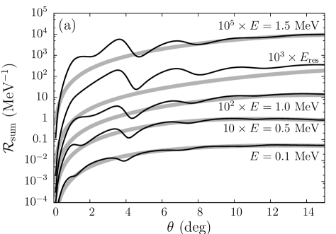
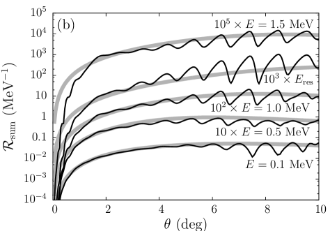
Figure 11: Change of the ratio with the energy $E$ in the $c$-$f$ continuum. (a) ¹¹Be on C at 67 MeV/nucleon; (b) ¹¹Be on Pb at 69 MeV/nucleon. For convenience, each ratio has been multiplied by a factor.

For the heavy target, the rise of the DEA ratio at forward angles is slower compared to its REB prediction (see Fig. 11(b)). As explained in Sec. IV.3, this slower rise is due to the adiabatic approximation made in the REB. Accordingly, the agreement between the dynamical calculation and the form factor $|F_{E,0}|^{2}$ at forward angles gets worse with increasing excitation energy. This discrepancy is not observed on the light target for which the adiabatic approximation is well suited.

Of particular interest is the case where the final state is a resonance. The calculations displayed in Fig. 11 do not show unusual effects at $E_{\rm res}$. The ratio rises slightly faster at large scattering angles and its residual oscillations are slightly larger than off-resonance. These more significant departures from the REB prediction might be seen experimentally and could hence be used to spot resonant structures in the continuum of exotic nuclei. However such a feature is more clearly observed in energy distributions measured after breakup on a light target Fukuda et al. (2004); Capel et al. (2004).

This analysis shows that although the agreement between the DEA ratio and its REB prediction remains fair, the ratio method would be better applied at low energy $E$ in the projectile continuum and off resonance. In the case studied here, the discrepancy remains small up to a ¹⁰Be-$n$ energy $E\sim 0.5$ MeV.

VI Conclusion and prospects

A new observable for halo nuclei has been studied in detail. It consists of the ratio of the breakup angular distribution and the summed angular distribution including elastic, inelastic and breakup. We show that realistic calculations of this observable closely follow predictions by the REB model. The latter neglects the neutron-target interaction and the excitation energy of the projectile. In this work we have explored the small discrepancies that exist between dynamical calculations and their REB predictions: the DEA ratio exhibits residual oscillations and rises more slowly than the REB at very forward angles for Coulomb-dominated processes. The residual oscillations are caused by the additional kick the neutron feels due to its interaction with the target $U_{nT}$. The difference observed at forward angles on heavy targets is due to the adiabatic approximation made in the REB, which is incompatible with the long range of the Coulomb interaction. Nevertheless, these discrepancies remain small indicating that most of the dependence on the reaction mechanism is removed by taking this ratio of cross sections. Therefore the cross section ratio is an optimal tool to study the structure of exotic nuclei.

We next analyze the structure information contained in the cross section ratio. Our results show that the ratio is extremely sensitive to the binding energy of the halo and the angular momentum of the halo orbital. While binding energy and angular momentum can be unequivocally extracted, an experimental error of a few percents would be necessary for learning about the details of the radial behavior of the halo. Very accurate data could constrain simultaneously the asymptotic normalization coefficient as well as the internal behavior of the radial wave function. One advantage of the ratio method is that it provides an additional control variable, the energy of the continuum bin, which can be tuned to be most appropriate to the case under study. Although the method works best when the excitation in the continuum is small, we show that even at 1.5 MeV useful results can be obtained.

Thanks to its independence of the reaction mechanism, the cross section ratio enables us to probe in-depth the structure of one-neutron halo nuclei and brings out information inaccessible to any other reaction observable. According to our analysis, the ratio method works both on light and heavy targets. It gives better results at high beam energy and for loosely-bound projectiles, for which the adiabatic approximation is more reliable.

Appendix A Other ratios

We have also considered ratios obtained by integrating over the relative energy of the breakup fragments. This could be of interest due to low statistics of the energy distribution of the breakup fragments or other experimental constraints. The resulting expressions are denoted by ${\cal R}_{\rm\int\!\!el}$ and ${\cal R}_{\rm\int\!\!sum}$ and are defined by

$${\cal R}_{\rm\int\!\!el}(\mbox{\boldmath$Q$}) = \frac{\int d\sigma_{\rm bu}/dEd\Omega\;dE}{d\sigma_{\rm el}/d\Omega}$$ (24)

$$\stackrel{{\scriptstyle\rm(REB)}}{{=}} \frac{1-(|F_{0,0}(\mbox{\boldmath$Q$})|^{2}+\sum_{i>0}|F_{i,0}(\mbox{\boldmath$Q$})|^{2})}{|F_{0,0}(\mbox{\boldmath$Q$})|^{2}},$$ (25)

and

$${\cal R}_{\rm\int\!\!sum}(\mbox{\boldmath$Q$}) = \frac{\int d\sigma_{\rm bu}/dEd\Omega\;dE}{d\sigma_{\rm sum}/d\Omega}$$ (26)

$$\stackrel{{\scriptstyle\rm(REB)}}{{=}} 1-(|F_{0,0}(\mbox{\boldmath$Q$})|^{2}+\sum_{i>0}|F_{i,0}(\mbox{\boldmath$Q$})|^{2}).$$ (27)

In this case however, all configurations of the final breakup fragments are contributing. As detailed in Secs. IV.3 and V.4, the higher the relative energy between the breakup fragments $E$, the less valid is the adiabatic approximation assumed in the REB model. Therefore, we found that neither ${\cal R}_{\rm\int\!\!el}$ (24) nor ${\cal R}_{\rm\int\!\!sum}$ (26) are useful.

Appendix B Two-body interactions

Most of the calculations presented in this text have been performed using the DEA Baye et al. (2005); Goldstein et al. (2006) with the description of ¹¹Be developed in LABEL:capel04 and the optical potentials of LABEL:dea2. This appendix details the form-factors of these potentials and lists their parameters used in this study.

The projectile model is based on the two-body description presented in Sec. II.1. The $V_{cn}$ potential contains a central term plus a spin-orbit coupling term

$$V_{cn}(\mbox{\boldmath$r$})=V_{0}f(r,R_{0},a)+V_{LS}\ \mbox{\boldmath$l$}\cdot\mbox{\boldmath$s$}\ \frac{1}{r}\frac{d}{dr}f(r,R_{0},a),$$ (28)

with the Woods-Saxon form factor

$$f(r,R_{0},a)=\left[1+\exp\left(\frac{r-R_{0}}{a}\right)\right]^{-1}$$ (29)

of radius $R_{0}$ and diffuseness $a$. In Eq. (28), $l$ is the relative orbital angular momentum between the core and the valence neutron, and $s$ is the spin of the neutron. For completeness, we list in Table 1 the parameters of the $c$-$n$ potentials used in this analysis. The first two rows contain the original potential of LABEL:capel04 for ¹¹Be (for even and odd orbital angular momenta). This potential reproduces the experimental binding energy $E_{0}=-0.5$ MeV in the $1s_{1/2}$ orbital to describe the $1/2^{+}$ ground state of ¹¹Be. For the $1/2^{-}$ excited state, we take the $0p_{1/2}$ bound state of the potential, which requires a different depth $V_{0}$ for even and odd partial waves.

The continuum wave functions appearing in Eq. (14) are obtained with the $V_{cn}$ potential. Note that the $5/2^{+}$ resonance at 1.274 MeV in the ¹⁰Be-$n$ continuum, is reproduced in the $d_{5/2}$ partial wave with the original potential of Table 1 Capel et al. (2004). The other lines of Table 1 contain the parameters used for the calculations presented in Figs. 8, 9, and 10. The last line correspond to the potential used to describe ¹⁹C in the calculations presented in Fig. 7. The potentials are labeled as the corresponding curves in the figures. In most of the ¹¹Be calculations the parameters listed in Table 1 are used only in the ground-state partial wave, the others, including the continuum wave functions, being described by the “Original” potential. Only in the $0p_{1/2}$ and $0d_{5/2}$ cases do we use the same potential in all partial waves. In the ¹⁹C case, all partial waves are described using the same potential.

	$V_{0}$	$V_{LS}$	$R_{0}$	$a$
	(MeV)	(MeV fm2)	(fm)	(fm)
Original (even $l$)	62.52	21.00	2.585	0.6
Original (odd $l$)	39.74	21.00	2.585	0.6
$E_{0}=-50$ keV	57.91	21.00	2.585	0.6
$E_{0}=-5$ MeV	80.00	21.00	2.585	0.6
$R=1$ fm	210.19	21.00	1	0.6
$R=4$ fm	30.915	21.00	4	0.6
$0s_{1/2}$	11.191	21.00	2.585	0.6
$0p_{1/2}$	40.861	21.00	2.585	0.6
$0d_{5/2}$	74.162	0.00	2.585	0.6
18C-$n$	42.161	14.00	3.24	0.62

Table 1: Parameters of the core-$n$ potentials (28).

The nuclear part of the optical potentials used to simulate the interaction between the projectile constituents and the targets contains real and imaginary volume terms and an imaginary surface term

$$U_{xT}=-Vf(r,R_{r},a_{r})$$ (30)

$$- i\left[Wf(r,R_{i},a_{i})+W_{d}\ a_{i}\frac{d}{dr}f(r,R_{i},a_{i})\right].$$

The Coulomb part of $U_{cT}$ is simulated by the potential due to a uniformly charged sphere of radius $R_{C}$. The parameters of the optical potentials used in this study are listed in Table 2. We follow LABEL:dea2 for the choices of most of these optical potentials. For $U_{nT}$ we use the Becchetti and Greenlees parameterization Becchetti and Greenlees (1969), for the Pb target. For the carbon target, we follow LABEL:capel04 and use the $p$-C potential of Comfort and Karp Comfort and Karp (1980). The ¹⁰Be-Pb potentials are obtained from $\alpha$-Pb potentials by merely rescaling the radius for an $A=10$ projectile Bonin et al. (1985); Goldberg et al. (1973). For the ¹⁰Be-C potential, we follow LABEL:capel04 and use the potential developed by Al-Khalili, Tostevin and Brooke that fits the elastic scattering of ¹⁰Be on C at 49.3 MeV/nucleon Al-Khalili et al. (1997). The ¹⁸C-Pb interaction is derived from the potential of LABEL:Bue84 that fits the ¹³C-Pb elastic scattering at 390 MeV.

$P$	$T$	Energy	$V$	$R_{r}$	$a_{r}$	$W$	$W_{d}$	$R_{i}$	$a_{i}$	$R_{C}$	Ref.
		(MeV/nucleon)	(MeV)	(fm)	(fm)	(MeV)	(MeV)	(fm)	(fm)	(fm)
$n$	Pb	69	29.46	6.93	0.75	13.4	0	7.47	0.58	-	Becchetti and Greenlees (1969)
		40	38.423	6.93	0.75	7.24	1.846	7.47	0.58	-	Becchetti and Greenlees (1969)
		100	44.823	6.93	0.75	2.84	21.846	7.7	0.58	-	Becchetti and Greenlees (1969)
		67	29.78	6.93	0.75	13.18	0	7.47	0.58	-	Becchetti and Greenlees (1969)
	C	67	30.9	2.75	0.623	7.82	0	3.18	0.667	-	Comfort and Karp (1980)
10Be	Pb	69	79.5	8.08	0.893	36.5	0	8.16	0.846	8.08	Bonin et al. (1985)
		40	155	8.17	0.667	23.26	0	9.42	0.733	8.92	Goldberg et al. (1973)
		100	71.5	7.92	0.93	57.6	0	7.76	0.934	8.08	Bonin et al. (1985)
	C	67	123	3.33	0.8	65	0	3.47	0.8	5.33	Al-Khalili et al. (1997)
18C	Pb	67	200.0	5.39	0.9	76.2	0	6.58	0.38	5.92	Bue84

Table 2: Parameters of the optical potentials (30) used to simulate the interaction between the targets and projectile fragments $n$, and ¹⁰Be or ¹⁸C.