Attractor solutions in scalar-field cosmology

Abstract

Models of cosmological scalar fields often feature “attractor solutions” to which the system evolves for a wide range of initial conditions. There is some tension between this well-known fact and another well-known fact: Liouville’s theorem forbids true attractor behavior in a Hamiltonian system. In universes with vanishing spatial curvature, the field variables $\phi$ and $\dot{\phi}$ specify the system completely, defining an effective phase space. We investigate whether one can define a unique conserved measure on this effective phase space, showing that it exists for $m^{2}\phi^{2}$ potentials and deriving conditions for its existence in more general theories. We show that apparent attractors are places where this conserved measure diverges in the $\phi$-$\dot{\phi}$ variables and suggest a physical understanding of attractor behavior that is compatible with Liouville’s theorem.

I Introduction

Two of the favorite moves in the repertoire of the modern theoretical cosmologist are (1) positing one or more scalar fields whose energy density exerts an important influence on the evolution of the universe and (2) claiming (or at least aspiring to be able to claim) that certain conditions or behaviors qualify as “natural”. These tendencies meet in the notion of cosmological attractors: dynamical conditions under which evolving scalar fields approach a certain kind of behavior without finely-tuned initial conditions Guo et al. (2003); Ureña-López and Reyes-Ibarra (2009); Belinsky et al. (1985); Piran and Williams (1985); Ratra and Peebles (1988); Liddle and Lyth (2000); Liddle et al. (1994); Kiselev and Timofeev (2008); Ferreira and Joyce (1998); Downes et al. (2012); Khoury and Steinhardt (2011); Clesse et al. (2009), whether in inflationary cosmology or late-time quintessence models. In dynamical systems theory, attractor behavior describes situations where a collection of phase-space points evolve into a certain region and never leave. This is incompatible with Liouville’s theorem, which states that the volume of a region of phase space is invariant under time evolution. Hamiltonian systems, of which scalar-field cosmologies (Einstein’s equation plus a dynamical scalar field, restricted to homogeneous configurations) are examples, obey Liouville’s theorem, and therefore cannot support true attractor behavior.

So what is going on? In this paper we reconcile the appearance of attractor solutions in scalar-field cosmologies with their apparent mathematical impossibility by making two points. First, we point out the fact (well-known, although rarely stated explicitly) that the combined gravity/scalar-field equations exhibit an apparently accidental simplification in the case of flat universes. This simplification allows us to express the complete evolution in terms of an effective two-dimensional “phase space” with coordinates $\phi$ and $\dot{\phi}$, even though the true phase space is four-dimensional (since the scale factor and its conjugate momentum are independent variables). Of course, $\phi$ and $\dot{\phi}$ aren’t canonical coordinates on phase space, so the measure ${\rm d}\dot{\phi}\wedge{\rm d}\phi$ isn’t very physically meaningful.

Our second point is that it is seemingly possible to define a conserved measure on the $\phi$-$\dot{\phi}$ effective phase space, although this measure looks very different from ${\rm d}\dot{\phi}\wedge{\rm d}\phi$. We cannot rigorously prove its existence in general, but we can show that it corresponds to a Lagrangian on effective phase space if it does exist; in the simple example of a canonical scalar field with a quadratic potential, we show that a unique measure on effective phase space exists and derive some of its properties. By construction, there can be no “attractor” solutions with respect to this measure. Nevertheless, we suggest there is a relevant sense in which attractor solutions are physically meaningful, if certain functions of the phase-space variables are directly observable. Finally, we comment on the connection between this classical analysis and the boundary induced on phase space by the Planck scale.

II Phase Space, Measures, and Attractors

We start by reviewing scalar-field cosmology in phase space, following Gibbons, Hawking, and Stewart (1987) (GHS). There are subtleties due to the fact that GR is a constrained system. In this section, we also discuss the intuitive idea of an attractor and contrast it with Hamiltonian behavior.

Because a phase space $\Gamma$ of dimension $2n$ is a symplectic manifold, there is a closed two-form defined on $\Gamma$,

$$\omega=\sum_{i=1}^{n}\mathrm{d}p_{i}\wedge\mathrm{d}q^{i}.$$ (1)

This symplectic form defines the Liouville measure,

$$\Omega=\frac{\left(-1\right)^{n\left(n-1\right)/2}}{n!}\omega^{n}.$$ (2)

Liouville’s theorem from classical mechanics states that this measure is conserved along the Hamiltonian flow vector $X_{\mathcal{H}}$. That is, given trajectories that initially cover some region $S\subset\Gamma$ and that evolve under $X_{\mathcal{H}}$ to cover region $S^{\prime}$, we have

$$\int_{S}\Omega=\int_{S^{\prime}}\Omega.$$ (3)

Equivalently, the Lie derivative of $\Omega$ vanishes along $X_{\mathcal{H}}$,

$$\pounds_{X_{\mathcal{H}}}\Omega=0.$$ (4)

Because the metric component $g_{00}$ is not a propagating degree of freedom in the Einstein–Hilbert action, general relativity is a constrained system, in which the Hamiltonian $\mathcal{H}$ is set to a boundary-condition-dependent constant along physical trajectories. That is, trajectories are confined to a hypersurface in $\Gamma$ of dimension $2n-1$ for which $\mathcal{H}=\mathcal{H}_{\star}$; we will call this the Hamiltonian constraint surface,

$$C=\Gamma/\left\{\mathcal{H}=\mathcal{H}_{\star}\right\}.$$ (5)

The Hamiltonian flow vector, describing Hamiltonian evolution of trajectories in $C$, is

$$X_{\mathcal{H}}=\frac{\partial\mathcal{H}}{\partial p_{i}}\frac{\partial}{\partial q^{i}}-\frac{\partial\mathcal{H}}{\partial q^{i}}\frac{\partial}{\partial p_{i}},$$ (6)

where $(q^{i},p_{i})$ are the canonical coordinates and their conjugate momenta. The space of trajectories (as opposed to states) can be defined by taking the quotient

$$M=C/X_{\mathcal{H}}.$$ (7)

Previously, Gibbons et al. (1987) contructed the unique measure on $M$ for FRW universes. The GHS measure is unique in that it is positive, independent of parametrization, and respects the symmetries of the problem without introducing additional structures. It is obtained from the symplectic form $\omega$ by identifying the $n$th coordinate of phase space $\Gamma$ as time $t$, so that

$$\omega=\tilde{\omega}+\mathrm{d}\mathcal{H}\wedge\mathrm{d}t=\sum_{i=1}^{n-1}\mathrm{d}p_{i}\wedge\mathrm{d}q^{i}+\mathrm{d}\mathcal{H}\wedge\mathrm{d}t.$$ (8)

The corresponding measure, a $\left(2n-2\right)$-form, is

$$\Theta=\frac{\left(-1\right)^{\left(n-1\right)\left(n-2\right)/2}}{\left(n-1\right)!}\tilde{\omega}^{n-1}.$$ (9)

The metric describing an FRW universe is

$$\mathrm{d}s^{2}=-N^{2}\mathrm{d}t^{2}+a^{2}\left(t\right)\left(\frac{\mathrm{d}r^{2}}{1-\kappa r^{2}}+r^{2}\mathrm{d}\Omega^{2}\right),$$ (10)

where $a\left(t\right)$ is the scale factor, normalized to unity at some time $t_{0}$, and $N$ is the lapse function. The curvature parameter $\kappa\in\mathbb{R}$ has dimensions of $\left[\mathrm{length}\right]^{-2}$. We may also define $k=\kappa R_{0}^{2}\in\left\{0,\pm 1\right\}$, where $R_{0}$ is the radius of curvature of the universe when $a(t_{0})=1$.

     

Figure 1: Apparent attractor solutions for an $m^{2}\phi^{2}$ potential, with equation of motion $\ddot{\phi}+\sqrt{3/2}\sqrt{m^{2}\phi^{2}+\dot{\phi}^{2}}\dot{\phi}+m^{2}\phi=0$. Solid: the apparent attractors; dotted: numerical solutions for random initial conditions. Plots are in $\phi$-$\dot{\phi}$ space, in units where $M_{\mathrm{Pl}}=1$; the scalar mass is chosen to be $m=0.2M_{\mathrm{Pl}}$. At large field values, the solutions are approximated by the lines $\dot{\phi}=\pm\sqrt{2/3}m$, while for small field values, all solutions converge on the origin.

     

Figure 2: Numerical solution for evolution of an FRW universe with an $m^{2}\phi^{2}$ potential, with initial conditions $(\phi,\dot{\phi})=(6,0.25)$ at $a\left(t=0\right)=1$, plotted in $(\phi,p_{\phi})$ coordinates, where $p_{\phi}=a^{3}\dot{\phi}$ is the canonical momentum conjugate to $\phi$. Units are chosen such that $M_{\mathrm{Pl}}=1$, with the scalar mass $m=0.2M_{\mathrm{Pl}}$. The apparent attractor behavior seen in Fig. 1 disappears in these coordinates.

Studying the dynamics of the FRW scale factor coupled to some matter source is known as the minisuperspace approximation. The minisuperspace Lagrangian for gravity plus a scalar field with potential $V\left(\phi\right)$ is

$$\mathcal{L}=3M_{\mathrm{Pl}}^{2}\left(Na\kappa-\frac{a\dot{a}^{2}}{N}\right)+a^{3}\left[\frac{\dot{\phi}^{2}}{2N}-NV\left(\phi\right)\right].$$ (11)

The canonical momenta, defined as $p_{i}=\partial\mathcal{L}/\partial\dot{q}^{i}$, are

$$p_{N}=0,\;p_{a}=-6N^{-1}M_{\mathrm{Pl}}^{2}a\dot{a},\;\mathrm{and}\;\;p_{\phi}=N^{-1}a^{3}\dot{\phi}.$$ (12)

Note that $N$ is a Lagrange multiplier: it is non-dynamical and will not be a part of the phase space. Performing a Legendre transformation, the Hamiltonian, in units where $M_{\mathrm{Pl}}=\sqrt{\hbar c/8\pi G}=1$, is

$$\mathcal{H} =N\left[-\frac{p_{a}^{2}}{12a}+\frac{p_{\phi}^{2}}{2a^{3}}+a^{3}V\left(\phi\right)-3a\kappa\right]$$ (13)

$$=-3a^{3}N\left\{\left(\frac{\dot{a}}{a}\right)^{2}+\frac{\kappa}{a^{2}}-\frac{1}{3}\left[\frac{1}{2}\dot{\phi}^{2}+V\left(\phi\right)\right]\right\}.$$

The equation of motion for $N$ sets it equal to an arbitrary constant, which we choose to be unity henceforth. Varying the action with respect to $N$ gives the Hamiltonian constraint for FRW universes, $\mathcal{H}_{\star}=0$, which is equivalent to the Friedmann equation,

$$H^{2}=\frac{1}{3}\left[\frac{1}{2}\dot{\phi}^{2}+V\left(\phi\right)\right]-\frac{\kappa}{a^{2}},$$ (14)

where the Hubble parameter is $H\equiv\dot{a}/a$. Thus, $\Gamma$ is four-dimensional, with $(\phi,\;p_{\phi},\;a,\;p_{a})$ being a possible parametrization. The Hamiltonian constraint surface $C$, once a value of $\kappa$ is chosen, is three-dimensional. The space of trajectories $M$ is two-dimensional. The GHS measure can be written as the Liouville measure with the Hamiltonian constraint:

$$\Theta=\left.\left(\mathrm{d}p_{a}\wedge\mathrm{d}a+\mathrm{d}p_{\phi}\wedge\mathrm{d}\phi\right)\right|_{\mathcal{H}=0}.$$ (15)

A true attractor in phase space can be thought of as a region toward which phase-space trajectories converge when plotted in canonical coordinates. More formally, an attractor is defined Milnor (1985) as a region $A\subset\Gamma$ with the following properties:

1. $A$ is compact;

2. Given a trajectory $\{\mathcal{P}(t,x_{0})\}\subset\Gamma$ beginning at $\mathcal{P}(t_{0},x_{0})=x_{0}\in A$, $\mathcal{P}(t,x_{0})\in A$ for all $t>t_{0}$;

3. There exists a basin of attraction, a neighborhood $B$ of $A$ such that for all $x_{B}\in B$ and for any neighborhood $N$ of $A$, there exists $t_{N}$ such that $\mathcal{P}(t,x_{B})\in N$ for all $t>t_{N}$;

4. Properties 2. and 3. are not satisfied by any $A^{\prime}\subsetneq A$.

There are other, related, definitions of attractors in the mathematical literature Auslander et al. (1964); in particular, a definition in terms of Lyapunov stability is possible (cf. Sec. VI, below).

An immediate consequence of Liouville’s theorem is that no true attractor can exist in the phase space of a system described by a Hamiltonian Gibbs (1902); see also Ref. Misner et al. (1973), Sec. 22.6. Intuitively, if a bundle of trajectories converges along a particular axis in phase space in a given coordinate system, it must compensatingly spread out along other axes, to conserve the total phase-space measure. Though we may wish to describe such behavior as an “attractor”, it is always possible to remove this apparent convergence by a canonical change of coordinates: in essence, there is no coordinate-independent notion of an attractor in the full four-dimensional phase space describing scalar-field cosmology in an FRW universe Tseng (2013).

Despite the fact that it does not rigorously exist, however, the intuitive idea of an attractor appears in the literature on scalar field cosmology, though a definition of what is meant by an “attractor” is often left implicit. This often occurs as a result of plotting trajectories in some non-canonical phase-space variables, most commonly $\phi$ versus $\dot{\phi}$ Guo et al. (2003); Ureña-López and Reyes-Ibarra (2009); Downes et al. (2012). However, as one can see in Figs. 1 and 2, apparent attractor behavior in $(\phi,\dot{\phi})$ coordinates need not correspond to attractor behavior when plotted in $(\phi,p_{\phi})$. Furthermore, recall that the full phase space $\Gamma$ is four-dimensional, not two-dimensional: $a$ and $p_{a}$ are suppressed in Figs. 1 and 2, and initially nearby trajectories would generally spread in these variables. In other papers, the notion of an “attractor” is used in a manifestly coordinate-dependent manner, with respect to some physical observables that either become smaller with time Khoury and Steinhardt (2011) or for which differences between initially different trajectories vanish rapidly in some particular coordinates Liddle and Lyth (2000); Liddle et al. (1994); Kiselev and Timofeev (2008).

It is easy to see why such behavior is described as attractor-like: one simply looks at the plots, perhaps implicitly assuming a “graph paper measure” $\mathrm{d}\dot{\phi}\wedge\mathrm{d}\phi$. Though this assumption seems natural, it is a coordinate-dependent artifact, as $\phi$ and $\dot{\phi}$ are not canonically conjugate. It is our aim in this work to make all of these notions more rigorous, examining both the issue of the measure on the space of field variables and the definition of apparent attractor-like behavior. Our results should help to create a common, more mathematically valid, and less ad hoc language for comparing results between different models of scalar-field cosmology.

III Effective Phase Space for a Single Scalar Field

In this section, we identify a sense in which $\phi$ and $\dot{\phi}$, though not canonically conjugate, are special coordinates for universes with zero spatial curvature. That is, we will show that the full four-dimensional phase space $\Gamma$ is larger than necessary to fully capture the dynamics of scalar field cosmology for flat universes; $\phi$-$\dot{\phi}$ space can be regarded as an effective phase space, in a sense that will be made precise. We proceed first by defining the notion of a vector field invariant map, making as general and coordinate-independent definitions as possible. In essence, given a map between two manifolds and a vector field on the first manifold, the map is vector field invariant if it provides a way of uniquely specifying a vector field on the second manifold. We will find that the map from $\Gamma$ to $\phi$-$\dot{\phi}$ space for flat universes is vector field invariant with respect to the Hamiltonian flow vector.

III.1 Vector field invariant maps

Before investigating whether there is a sense in which the non-canonical coordinates $(\phi,\dot{\phi})$ constitute a parametrization with any special mathematical properties, we first require some definitions and notation. Given two manifolds $M$ and $N$, a mapping $\psi:\,M\rightarrow N$, and $f\in\mathcal{F}\left(N\right)$, where $\mathcal{F}\left(N\right)$ is the space of smooth real-valued functions with domain $N$, the pullback $\psi^{\star}:\,\mathcal{F}\left(N\right)\rightarrow\mathcal{F}\left(M\right)$ of $f$ by $\psi$ is defined by:

$$\psi^{*}f=\left(f\circ\psi\right):\,M\rightarrow\mathbb{R}.$$ (16)

We can think of $f$ as specifying a coordinate on $N$ and the pullback as specifying a coordinate on $M$. Now, at a given point $p\in M$, we may regard a vector $X\left(p\right)$ as a function $X_{p}:\,\mathcal{F}\left(M\right)\rightarrow\mathbb{R}$. If we think of $g\in\mathcal{F}\left(M\right)$ as specifying a coordinate (also called $g$) on $M$, then $X_{p}\left(g\right)$ gives the value of the $g$-component of the vector at $p$. A vector field $X$ on $M$ is the assignment of a vector $X_{p}$ to each point $p\in M$ in a continuous and smooth fashion. Given the map $\psi:\,M\rightarrow N$ and a function $f:\,N\rightarrow\mathbb{R}$, the pushforward of $X$ at $\psi\left(p\right)\in N$ is

$$\left(\psi_{*}X\right)_{\psi\left(p\right)}\left(f\right)=X_{p}\left(\psi^{*}f\right).$$ (17)

We note that the pushforward $\psi_{*}$ is a map from the tangent space at $p$, $T_{p}M$, into $T_{\psi(p)}N$ and that $\psi_{*}X:\,\mathcal{F}\left(N\right)\rightarrow\mathbb{R}$. In this sense, we can write $\psi_{*}\left(X\right)=X\circ\psi^{*}$. For further reference, see Appendix C of Wald (1984) and Appendix A of Carroll (2004).

We may now define “vector field invariance”, a way of formalizing the idea that a many-to-one map creates a unique vector field. Suppose we have a map $\psi:\,M\rightarrow N$ and vector field $X$ on $M$. For each point $q\in N$, write the preimage in $M$ as $\psi^{-1}\left(q\right)=\{p\in M\;|\;\psi\left(p\right)=q\}$. Then say that the map $\psi$ is vector field invariant with respect to $X$ if for any function $f\in\mathcal{F}\left(N\right)$ and for all $q\in N$, $X_{p}(\psi^{*}f)=X_{p^{\prime}}(\psi^{*}f)$ for all $p,\,p^{\prime}\in\psi^{-1}\left(q\right)$. If a map $\psi$ is vector field invariant with respect to $X$, we may write $X_{p}(\psi^{*}f)=\tilde{X}_{q}(f)$ without ambiguity for $p\in\psi^{-1}\left(q\right)$. Then we have a unique vector field $\tilde{X}$ on $N$. We can say that $\tilde{X}$ is the vector field induced by $X$ on $N$ under the (vector field invariant) map $\psi$.

The images of integral curves that are distinct under a vector field invariant map do not intersect. If we have a vector field invariant map $\psi:\,M\rightarrow N$, where $M$ has vector field $X$, then the images of integral curves of $X$ are integral curves of $\tilde{X}$ in $N$. Therefore, by uniqueness, given two integral curves in $M$ not mapped onto each other in $N$ by $\psi$, their images in $N$ cannot intersect. If $M$ is the phase space for some Hamiltonian system and $\psi:\,M\rightarrow N$ is vector field invariant with respect to the Hamiltonian flow vector, one can therefore think of $N$ as an effective phase space.

III.2 A map for FRW universes

We will now show that, for scalar-field cosmology in a flat universe, the choice of $\phi$ and $\dot{\phi}$ as coordinates allows one to eliminate $a$ and $\dot{a}$ and thus reduce the dynamical phase space to two dimensions. Consider a map $\chi$ from the Hamiltonian constraint three-manifold $C$ to a two-manifold $K$, where $\chi^{-1}\left(q\right)$ is the set of all points in $C$ with equal values of $\phi$ and $\dot{\phi}$. That is, $K$ is isomorphic to $\phi$-$\dot{\phi}$ space. We will show that in a flat universe ($\kappa=0$) with a scalar field described by a potential $V\left(\phi\right)$ and a canonical kinetic term, the map $\chi$ is vector field invariant with respect to the Hamiltonian flow vector $X_{\mathcal{H}}$.

It is sufficient to exhibit one such map $\chi$, as all other maps such that the preimage of $q\in K$ is the set of all points in $C$ with equal values of $\phi$ and $\dot{\phi}$ can be obtained from $\chi$ via a bijection. Without loss of generality, we may therefore specify coordinates $(\phi,\,\dot{\phi},\,a,\,H)$ on the full phase space $\Gamma$, which are inherited by $C$, so that $C$ is parametrized by four coordinates related by the Hamiltonian constraint. Note, however, that none of our conclusions are dependent on choosing $a$ and $H$ as the other two coordinates. That is, the notion of vector field invariance of $\chi:\,C\rightarrow K$ is a statement only about $\phi$ and $\dot{\phi}$, independent of the other coordinates. With the Hamiltonian (13) and flow vector (6), we have

$$X_{\mathcal{H}}^{\left(\phi\right)} =\frac{p_{\phi}}{a^{3}},$$ (18)

$$X_{\mathcal{H}}^{\left(p_{\phi}\right)} =-a^{3}V^{\prime}\left(\phi\right),$$

$$X_{\mathcal{H}}^{\left(a\right)} =-\frac{p_{a}}{6a},$$

$$X_{\mathcal{H}}^{\left(p_{a}\right)} =-\frac{p_{a}^{2}}{12a^{2}}+\frac{3p_{\phi}^{2}}{2a^{4}}-3a^{2}V\left(\phi\right)+3\kappa.$$

Using the expressions for $p_{a}$ and $p_{\phi}$ in Eq. (12) to rescale and eliminate $a$ and $\dot{a}$ in favor of $\phi$ and $\dot{\phi}$, we have

$$X_{\mathcal{H}}^{(\phi)}= \dot{\phi},$$ (19)

$$X_{\mathcal{H}}^{(\dot{\phi})}= \frac{1}{a^{3}}X_{\mathcal{H}}^{(p_{\phi})}=-V^{\prime}\left(\phi\right),$$

$$X_{\mathcal{H}}^{(H)}= \!-\frac{1}{6a^{2}}X_{\mathcal{H}}^{(p_{a})}\!\!=\frac{1}{2}H^{2}\!-\!\frac{1}{4}\dot{\phi}^{2}\!+\!\frac{1}{2}V\!\left(\phi\right)\!-\!\frac{\kappa}{2a^{2}}.$$

Therefore, for $\kappa=0$, the $\phi$-, $\dot{\phi}$-, and $H$-components of the vector field are independent of $a$. Further, from the Friedmann equation (14), $H$ can be written as a function of $\phi$ and $\dot{\phi}$ for $\kappa=0$. Thus, for a flat universe, the $\phi$-, $\dot{\phi}$-, and $H$-components of the Hamiltonian vector field $X_{\mathcal{H}}$ can be written in terms of $\phi$ and $\dot{\phi}$ alone. This is the slightly more careful version of our previous statement that $\phi$ and $\dot{\phi}$ allow $a$ and $\dot{a}$ to be eliminated from the dynamics. Now, consider the map $\chi:\,C\rightarrow K$ defined by $\chi(a,\phi,\dot{\phi},H)=(\phi,\dot{\phi})$. Under such a map, the condition for vector field invariance for a given vector field $X$ is simply the condition that the $\phi$-, $\dot{\phi}$-, and $H$-components of $X$ can be written in terms of only $\phi$ and $\dot{\phi}$. Hence, we conclude that the map $\chi$ is vector field invariant with resepect to the Hamiltonian vector field $X_{\mathcal{H}}$ for a flat universe.

We have shown, for a universe of zero spatial curvature, that there is a sense in which $(\phi,\dot{\phi})$ become effective phase-space coordinates. This formalizes the intuitive idea that the equations of motion can be written purely in terms of these variables. There exists a vector field invariant map with respect to the Hamiltonian flow vector, from the full three-dimensional constraint surface $C$ to a two-dimensional manifold $K$: we find that $K$ is isomorphic to $\phi$-$\dot{\phi}$ space. This is a nontrivial property – it is not in general true, given a three-dimensional surface with a Hamiltonian vector field, that a vector field invariant mapping to a two-dimensional manifold exists. The criterion $\kappa=0$ is necessary for $(\phi,\dot{\phi})$ to be an effective phase space; indeed, trajectories can cross in $\phi$-$\dot{\phi}$ space if $\kappa\neq 0$. Furthermore, the projection of $\Gamma$ onto two canonical coordinates does not constitute construction of an effective phase space; this fact can be illustrated dramatically by considering orbits in $(\phi,p_{\phi})$ for an $m^{2}\phi^{2}$ potential (see Fig. 2). In this sense, $\phi$ and $\dot{\phi}$ are special coordinates with which to parametrize the phase space of scalar-field cosmology.

III.3 The geometrical picture

One can develop more intuition about the notion of vector field invariance by considering the geometry of the Hamiltonian constraint submanifold embedded in the full phase space, for a specific model with $V\left(\phi\right)=m^{2}\phi^{2}/2$. The four-dimensional phase space $\Gamma$ is foliated into three-dimensional Hamiltonian submanifolds $C$, each with a unique value of $\kappa$, with the Friedmann equation (14) giving the constraint.

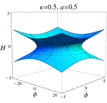
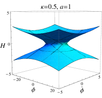
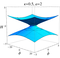
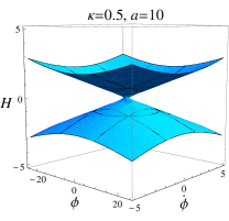
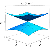
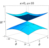
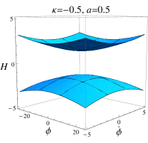
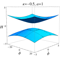
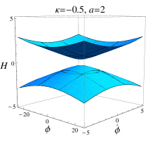
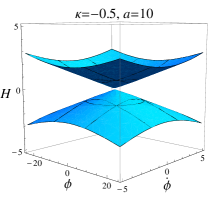
Figure 3: Plots of the Hamiltonian three-surface $C$ for $V\left(\phi\right)=m^{2}\phi^{2}/2$, in $(a,H,\phi,\dot{\phi})$ coordinates, at slices of various values of the scale factor $a$. Top row: $\kappa=0.5$, middle row: $\kappa=0$, bottom row: $\kappa=-0.5$. Units used are $M_{\mathrm{Pl}}=1$ and $m=0.2$.

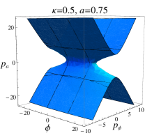
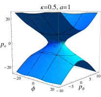
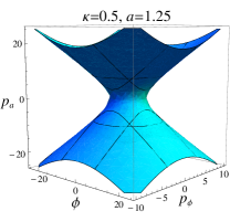
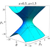
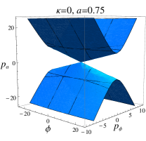
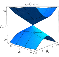
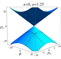
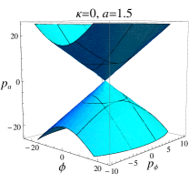
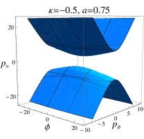
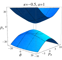
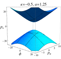
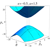
Figure 4: Plots of the Hamiltonian constraint manifold $C$ for $V\left(\phi\right)=m^{2}\phi^{2}/2$, in $(a,p_{a},\phi,p_{\phi})$ coordinates, in two-dimensional slices $C_{a}$ at various values of the scale factor $a$. Top row: $\kappa=0.5$, middle row: $\kappa=0$, bottom row: $\kappa=-0.5$. Units used are $M_{\mathrm{Pl}}=1$ and $m=0.2$.

Consider a Hamiltonian submanifold $C$ for some choice of curvature $\kappa$. Restricted to a particular value of the scale factor $a$, the Hamiltonian submanifold becomes a two-dimensional surface $C_{a}$ immersed within a three-dimensional space $\Gamma_{a}$. We can think of $C$ as being the disjoint union of the $C_{a}$. Formally speaking, $C$ is formed by the fibration of the family of manifolds $C_{a}$ over the positive real line $\mathbb{R}_{+}$ parametrized by $a$: in general, this produces a non-factorizable three-manifold within $\Gamma$, since the $C_{a}$ are often different in size and shape for different values of $a$. As one can see in Fig. 3, all the $C_{a}$ are the same if $\kappa=0$. This is due to the fact that for the choice $\kappa=0$, the Hamiltonian constraint (14) is independent of $a$ in $(a,H,\phi,\dot{\phi})$ coordinates:

$$H^{2}=\frac{1}{3}\left[\frac{1}{2}\dot{\phi}^{2}+V\left(\phi\right)\right].$$ (20)

More precisely, parametrizing $C_{a}=\Gamma_{a}\cap C$ with the other three coordinates on $\Gamma$ (excluding $a$), we find that, for $\kappa=0$, $C_{a}$ contains the same set of points, a cone in $\Gamma_{a}$, regardless of the choice of $a$. Hence, one can pick a two-manifold $C_{a_{\star}}$ for any choice of scale factor $a_{\star}$ and find that $C$ is a product space: $C=C_{a_{\star}}\times\mathbb{R}_{+}$. This is the sense in which $a$ ceases to be a dynamical variable for flat universes.

As previously, let $K\cong\mathbb{R}^{2}$ denote $\phi$-$\dot{\phi}$ space and consider the vector field invariant map $\chi:\,C\rightarrow K$ defined by $\chi(a,H,\phi,\dot{\phi})=(\phi,\dot{\phi})$, where $C$ is the Hamiltonian submanifold for a flat universe. More generally, we could let $K$ be any space isomorphic to $\phi$-$\dot{\phi}$ space and let $\chi$ be any function for which the preimage of a point in $K$ is the set of all points in $C$ with a particular value of $\phi$ and $\dot{\phi}$. It was previously shown that $\chi$ is vector field invariant with respect to the Hamiltonian flow vector $X_{\mathcal{H}}$. From Fig. 3 we can see why this is true. The Hamiltonian flow vector describes a vector field on $C$; on each manifold $C_{a}$, the $H$-, $\phi$-, and $\dot{\phi}$-components of $X_{\mathcal{H}}$ give a vector field, which we can imagine describing flow tangent to each of the slices shown in Fig. 3. The projection of the vector field from a slice $C_{a}$ down into the horizontal plane in Fig. 3 corresponds to the pushforward of the vector field from $C_{a}$ to $K$. If this vector field in $K$ is the same no matter which slice $C_{a}$ we chose, then $\chi$ is vector field invariant with respect to $X_{\mathcal{H}}$. This is manifestly true for the flat universe case, because $C$ factors as shown above. It is also clear from Fig. 3 that this is not true for $\kappa\neq 0$: the manifold $C_{a}$ changes dramatically as $a$ is varied, so the vector field that we push forward to $K$ will be different for different $a$.

At this point we may ask again: is this property of $\phi$ and $\dot{\phi}$ really distinctive? That is, does a different choice of coordinates on $\Gamma$, say $(a,p_{a},\phi,p_{\phi})$ give the same result: a map of the form $\psi$ from $(a,p_{a},\phi,p_{\phi})$ to $(\phi,p_{\phi})$ that, provided $\kappa=0$, is vector field invariant with respect to $X_{\mathcal{H}}$? We saw in Fig. 2 that this is not the case, but it is useful to consider why vector field invariance fails for $\phi$-$p_{\phi}$ space from the geometrical point of view. As we see in Fig. 4, even in the $\kappa=0$ case, the partition of the manifold $C$ into $C_{a}$ yields an inequivalent set of points in $\Gamma_{a}$ for different values of $a$ when parametrized by $(p_{a},\phi,p_{\phi})$, so that $C$ is merely a fibration of the $C_{a}$ over $\mathbb{R}_{+}$. Another way of saying this is that in $(a,p_{a},\phi,p_{\phi})$ coordinates, $C$ is non-factorizable even in the $\kappa=0$ case. Hence, drawing components of the Hamiltonian flow vector field on the partition of $C$, we see that a projection into the $\phi$-$p_{\phi}$ plane will give a vector field that is different at different values of $a$: that is, $\psi:\,(a,p_{a},\phi,p_{\phi})\rightarrow(\phi,p_{\phi})$ is not vector field invariant with respect to $X_{\mathcal{H}}$. In this way, we have shown that the property of vector field invariance that $\chi$ possesses is non-trivial and not a generic property of any map from $C$ onto a two-dimensional manifold: $\phi$ and $\dot{\phi}$ are coordinates with a special property.

IV Constructing a Measure on Effective Phase Space

We now have in hand an effective phase space $K$ for flat scalar-field cosmology, namely, $\phi$-$\dot{\phi}$ space. Its properties are defined generally through the formalism of a vector field invariant map and it contains all of the dynamical variables describing the evolution of a flat FRW universe dominated by a scalar field. However, while $K$ captures the entire dynamics of the system (every point is part of a unique trajectory), it is not naturally a symplectic manifold, the coordinates $(\phi,\dot{\phi})$ are not canonically conjugate, and there is no reason to expect the naïve measure ${\rm d}\dot{\phi}\wedge{\rm d}\phi$ to be conserved. We now ask whether these features can be corrected, by finding a measure on this effective phase space that actually is conserved.

While the Liouville measure (15) is appropriate for the full phase space $\Gamma$, we are interested now in finding a measure on the effective phase space. Taking a constructive approach, we first examine the constraint imposed by conservation of the measure under Hamiltonian evolution of trajectories, calling such a measure a “conserved measure”. We then examine the question of whether the effective phase space itself has a Lagrangian description, that is, whether the equation of motion in terms of $\phi$ and $\dot{\phi}$ alone can be derived from a Lagrangian $\mathcal{L}_{K}$ defined on $K$. If such a Lagrangian exists, it allows us to define a conjugate momentum $\pi_{\phi}\equiv\partial\mathcal{L}_{K}/\partial\dot{\phi}$. The measure $\mathrm{d}\pi_{\phi}\wedge\mathrm{d}\phi$ on $K$ is then automatically conserved under the Hamiltonian flow. We show that the converse is also true; if there is a conserved measure, there is a corresponding Lagrangian description. Finally, for the special case of an $m^{2}\phi^{2}$ potential, we examine the behavior of the measure at early and late times and prove that the measure on $K$ exists.

IV.1 Conservation under Hamiltonian flow

As shown in Ref. Carroll and Tam (2010), the GHS measure (15) diverges for flat universes ($\kappa=0$); see also Ref. Gibbons and Turok (2008). Specifically, as $\Omega_{k}$, the fraction of the critical energy density parametrized by curvature, approaches zero, $\Theta\propto\left|\Omega_{k}\right|^{-5/2}$. In this sense, as Carroll and Tam (2010) note, the flatness problem in cosmology is illusory, a consequence of implicitly assuming a flat measure on the space of FRW solutions; all universes but a set of measure zero are spatially flat, according to the GHS measure. This divergence was briefly noted by Gibbons et al. (1987). The GHS measure is only well-defined for Hamiltonian systems with an odd number of constraints (i.e., the Hamiltonian submanifold corresponds to a single constraint). However, it is important to note that the specification of a flat universe does not increase the number of constraints, since this just amounts to selecting a particular value of $\kappa$ in Eq. (14). See discussion in Sec. III.3 for details of the phase-space topology.

Given the observed (near-)flatness of our own universe Ade et al. (2013), it is well-motivated to consider the question of the measure on the subspace of $\Gamma$ corresponding to flat universes. Because of its divergent behavior for $\kappa=0$, the GHS measure cannot help us in this case. Earlier attempts to regularize the measure, for example by considering an $\epsilon$-neighborhood around the zero-curvature Hamiltonian constraint surface Carroll and Tam (2010) or by identifying universes with similar curvatures Gibbons and Turok (2008) have not proven satisfactory; see also Refs. Schiffrin and Wald (2012); Hawking and Page (1988). A different approach seems to be required. As we have seen, the scale factor $a$ becomes non-dynamical for $\kappa=0$ and the scalar coordinates $\phi$ and $\dot{\phi}$ constitute an effective phase space, by virtue of the vector field invariant mapping discussed in Sec. III. Though the GHS and Liouville measures give us no information in this subspace, we can use the principles and reasoning of the full phase-space argument to motivate the treatment of the measure question on effective phase space. As noted in Sec. II, it is conventional to implicitly assume a flat measure $\mathrm{d}\dot{\phi}\wedge\mathrm{d}\phi$ in effective phase space when making statements about attractors, number of $e$-foldings, etc. Considering the measure question in effective phase space allows us to assess the validity of this assumption.

For simplicity of notation, let the vector field $\tilde{X}_{\mathcal{H}}$ induced from the Hamiltonian evolution vector $X_{\mathcal{H}}$ under the mapping $\chi:\,C\rightarrow K\cong(\phi,\dot{\phi})$ be written in $K$ as $\mathbf{v}$. Define $x=\phi$ and $y=\dot{\phi}$. The measure on a two-dimensional space is a two-form $\boldsymbol{\sigma}$, which we can always write as

$$\boldsymbol{\sigma}=f(x,y)\mathrm{d}x\wedge\mathrm{d}y$$ (21)

for some function $f(x,y)$. We seek a measure that is conserved with evolution along $\mathbf{v}$:

$$\pounds_{\mathbf{v}}\boldsymbol{\sigma}=\pounds_{\mathbf{v}}\left[f\left(x,y\right)\mathrm{d}x\wedge\mathrm{d}y\right]=0.$$ (22)

We can compactly express the condition (22) as the vector equation

$$\nabla\cdot\left(f\mathbf{v}\right)=0.$$ (23)

Note that this is equivalent to one of the Euler equations of fluid dynamics for a steady flow, $\partial\rho/\partial t=0$, where $\rho$ is the density of the fluid and $\mathbf{v}$ its velocity field:

$$\frac{\partial\rho}{\partial t}+\nabla\cdot\left(\rho\mathbf{v}\right)=0.$$ (24)

This is simply the statement of conservation of mass. Hence, our conserved two-form can be thought of as the density of fluid in a steady-flow system. The probability of a given bundle of trajectories is conserved under Hamiltonian evolution, just as the mass of a parcel of fluid is conserved as it flows.

For a single scalar with a canonical kinetic term, the vector field $\mathbf{v}$ can be found from $X_{\mathcal{H}}$ as follows. Setting $X_{\mathcal{H}}^{(p_{\phi})}$ given in Eq. (18) equal to $\partial_{t}p_{\phi}$ [recalling from Eq. (12) that $p_{\phi}=a^{3}\dot{\phi}$], we have the Klein–Gordon equation

$$\ddot{\phi}+3H\dot{\phi}+V^{\prime}\left(\phi\right)=0.$$ (25)

With $H$ as given by the Friedmann equation (the Hamiltonian constraint) (20), we have

$$\ddot{\phi}=-\sqrt{3}\dot{\phi}\sqrt{\frac{1}{2}\dot{\phi}^{2}+V\left(\phi\right)}-V^{\prime}\left(\phi\right)=v^{\dot{\phi}}.$$ (26)

The vector field in $\phi$-$\dot{\phi}$ space is therefore

$$\mathbf{v}=\left(y,\;-\sqrt{3}y\sqrt{V\left(x\right)+\frac{1}{2}y^{2}}-V^{\prime}\left(x\right)\right).$$ (27)

IV.2 Existence of a Lagrangian

We now have an equation of motion (26) for $\phi$, obtained from the Friedmann and Klein–Gordon equations and defined by a potential $V\left(\phi\right)$. We are looking for a Lagrangian on the effective phase space $K\cong\left(x,y\right)$ from which an equivalent equation of motion can be derived. One reason for considering a Lagrangian description is that the direct approach, i.e., finding a closed-form solution to the Euler equation (23) for the vector field (27), is highly nontrivial for a typical potential.

The existence of a Lagrangian given an equation of motion is a famous question known as the inverse problem of the calculus of variations, which was finally solved by Douglas (1941) in 1941. See Santilli (1978) for further reference. Suppose we have an equation of motion in a single variable

$$\ddot{x}=F\left(x,\dot{x}\right).$$ (28)

Then Douglas’ theorem states that there exists a Lagrangian for which the Euler–Lagrange equation gives the correct equation of motion (28) if and only if there exists a function $f$ satisfying the Helmholtz condition

$$\frac{\mathrm{d}f}{\mathrm{d}t}+\frac{\partial F}{\partial\dot{x}}f=0,$$ (29)

or equivalently, with $y=\dot{x}$,

$$\frac{\partial f}{\partial t}+\frac{\partial}{\partial x}\left(\dot{x}f\right)+\frac{\partial}{\partial y}\left(Ff\right)=0.$$ (30)

For the problem at hand, defining $\phi=x$ and $\dot{\phi}=y$ as before, Eq. (26) can be written

$$F\left(x,y\right)=-\sqrt{3}y\sqrt{\frac{1}{2}y^{2}+V\left(x\right)}-V^{\prime}\left(x\right)=\ddot{x}.$$ (31)

Noting from Eq. (27) that $\mathbf{v}=\left(y,\;F\right)$, we are able to write the Helmholtz condition in the form

$$\frac{\partial f}{\partial t}+\frac{\partial}{\partial x}\left(v^{x}f\right)+\frac{\partial}{\partial y}\left(v^{y}f\right)=\frac{\partial f}{\partial t}+\nabla\cdot\left(f\mathbf{v}\right)=0.$$ (32)

This is precisely the Euler equation for fluid flow (24), with $f$ taking the place of the density. If there is a measure $f\;\mathrm{d\dot{\phi}}\wedge\mathrm{d}\phi$ on $\phi$-$\dot{\phi}$ space conserved along the Hamiltonian flow vector, then $\nabla\cdot\left(f\mathbf{v}\right)=0$. Thus, we have proven the following:

There exists a Hamiltonian-flow conserved measure on $\phi$-$\dot{\phi}$ space if and only if the equation of motion $\ddot{\phi}+\sqrt{3}\dot{\phi}\sqrt{\dot{\phi}^{2}/2+V\left(\phi\right)}+V^{\prime}\left(\phi\right)=0$ possesses a Lagrangian description in effective phase space. More specifically, there exists a time-independent measure on $\phi$-$\dot{\phi}$ space if and only if the Helmholtz condition is satisfied by a time-independent function $f(\phi,\dot{\phi})$.

In other words, a Lagrangian description of the equation of motion (31) [cf. Eq. (26)] exists if and only if the Helmholtz condition (29) is satisfied. In turn, the Helmholtz condition is satisfied if and only if there is a function $f$ satisfying the Euler equation (24) for fluid flow with the Hamiltonian vector field (27). Whether or not there is such a function is difficult to establish in general, although we will give an argument in the case of $m^{2}\phi^{2}$ potentials.

IV.3 The conjugate momentum and the measure

If the Helmholtz condition (29) is satisfied, then the equation of motion can be written in the form

$$A\left(t,\phi,\dot{\phi}\right)\ddot{\phi}+B\left(t,\phi,\dot{\phi}\right)=0,$$ (33)

where

$$\frac{\partial B}{\partial\dot{\phi}}=\left(\frac{\partial}{\partial t}+\dot{\phi}\frac{\partial}{\partial\phi}\right)A.$$ (34)

Explicitly, given $f$ satisfying Eq. (32) and with $A=f(t,\phi,\dot{\phi})$ and $B=-f(t,\phi,\dot{\phi})\,F(\phi,\dot{\phi})$, where $F$ is given in Eq. (31), it can be shown that Eq. (34) is satisfied and that Eq. (33) corresponds to the correct equation of motion (26). Then as shown in Ref. Santilli (1978), the Lagrangian can be constructed explicitly:

$$\mathcal{L}_{K}\left(t,\phi,\dot{\phi}\right)=G\left(t,\phi,\dot{\phi}\right)+C\left(t,\phi\right),$$ (35)

where

$$G\!\left(t,\!\phi,\!\dot{\phi}\right) =\!\dot{\phi}\!\int_{0}^{1}\!\!\mathrm{d}\tau^{\prime}\!\!\left[\dot{\phi}\!\int_{0}^{1}\!\!\mathrm{d}\tau A\!\!\left(t,\!\phi,\!\tau\dot{\phi}\right)\right]\!\!\left(t,\!\phi,\!\tau^{\prime}\dot{\phi}\right),$$ (36)

$$C\!\left(t,\!\phi\right) =\!\phi\int_{0}^{1}\mathrm{d}\tau\,W\left(t,\!\tau\phi\right),\;\;\;\mathrm{and}$$

$$W\!\left(t,\!\phi\right) =\!-B-\frac{\partial G}{\partial\phi}+\frac{\partial^{2}G}{\partial\dot{\phi}\partial t}+\frac{\partial G}{\partial\phi\partial\dot{\phi}}\dot{\phi}.$$

We can then extract the momentum $\pi_{\phi}$ conjugate to $\phi$ in $\phi$-$\dot{\phi}$ space via

$$\pi_{\phi}=\frac{\partial\mathcal{L}_{K}}{\partial\dot{\phi}}=\frac{\partial G}{\partial\dot{\phi}}.$$ (37)

Then the Liouville measure on $\phi$-$\dot{\phi}$ space is

$$\mathrm{d}\pi_{\phi}\wedge\mathrm{d}\phi=\frac{\partial^{2}G}{\partial\dot{\phi}^{2}}\mathrm{d}\dot{\phi}\wedge\mathrm{d}\phi.$$ (38)

With $A=f$, it can be shown from Eq. (36) that $\partial_{\dot{\phi}}^{2}G=f$ and hence

$$\mathrm{d}\pi_{\phi}\wedge\mathrm{d}\phi=f\;\mathrm{d}\dot{\phi}\wedge\mathrm{d}\phi.$$ (39)

In the previous section, we demonstrated that finding a Lagrangian producing the equation of motion on $\phi$-$\dot{\phi}$ space was the same problem as constructing a Hamiltonian-flow conserved measure on that space. The result we have proven in this section states something stronger:

The natural Liouville measure $\mathrm{d}\pi_{\phi}\wedge\mathrm{d}\phi$ on effective phase space that one obtains from the effective Lagrangian, if it exists, is the same measure that one finds by explicitly constructing a nontrivial two-form $f\,\mathrm{d}\dot{\phi}\wedge\mathrm{d}\phi$ conserved under Hamiltonian evolution.

We note that these results are applicable to any single-field $V\left(\phi\right)$ model with canonical kinetic term, or with slight generalization, to any dynamical problem in a single variable.

V The Measure on Effective Phase Space for Quadratic Potentials

It is illustrative to explicitly investigate the behavior of the measure on effective phase space for a specific model,

$$V\left(\phi\right)=\frac{1}{2}m^{2}\phi^{2}.$$ (40)

Ideally, one would like to obtain a closed-form expression for the measure; however, solving the partial differential equation explicitly proves to be prohibitive. We obtain expressions for the behavior of the measure in two limits, $H\gg m$ and $H\ll m$, which can be viewed as corresponding to early and late times. Finally, we use the Cauchy–Kowalevski theorem to prove that a unique measure obeying the constraint (23) exists, up to overall normalization.

V.1 Constraining the behavior of the measure

It is convenient at this point to reparametrize the vector field in terms of polar coordinates. Again setting $x=\phi$ and $y=\dot{\phi}$, let

$$r=\sqrt{y^{2}+m^{2}x^{2}}=\sqrt{6}H$$ (41)

and

$$\tan\theta=\frac{y}{mx}.$$ (42)

Then the vector field (27) can be written as

$$\mathbf{v}=-\sqrt{\frac{3}{2}}r^{2}\sin^{2}\theta\;\boldsymbol{\hat{\mathbf{r}}}-\left(mr+\sqrt{\frac{3}{2}}r^{2}\sin\theta\cos\theta\right)\boldsymbol{\hat{\theta}},$$ (43)

where $\mathbf{\hat{r}}=\mathbf{\hat{x}}m^{-1}\cos\theta+\mathbf{\hat{y}}\sin\theta$ and $\boldsymbol{\hat{\theta}}=-\mathbf{\hat{x}}m^{-1}\sin\theta+\mathbf{\hat{y}}\cos\theta$ are unit vectors under the appropriate scaling of axes. The constraint (23) for a time-independent measure $f$ may be expressed as an explicit partial differential equation

$$0 =-\frac{1}{r}\sqrt{\frac{3}{2}}\sin^{2}\theta\partial_{r}\left(r^{3}f\right)$$ (44)

$$\hskip 10.00002pt\hskip 10.00002pt-m\partial_{\theta}f-\sqrt{\frac{3}{2}}r\partial_{\theta}\left(f\sin\theta\cos\theta\right).$$

V.1.1 Late universe limit

The late-universe, $H\rightarrow 0$ limit corresponds to $r\rightarrow 0$. Suppose first that $f$ does not diverge in this limit. Then as $\mathbf{v}\cdot\mathbf{\hat{r}}=-\sqrt{3/2}r^{2}\sin^{2}\theta<0$ for all $r$, $\theta$, it follows that for any circular disk $R$ of radius $r_{\star}$ centered at the origin,

$$\int_{R}\!\nabla\!\cdot\!\left(f\mathbf{v}\right)\!\mathrm{d}A =\oint_{\partial R}\!\!\left(f\mathbf{v}\right)\!\cdot\!\mathbf{\hat{n}}\mathrm{d}\ell$$ (45)

$$=-\sqrt{\frac{3}{2}}\int_{0}^{2\pi}\!\!f\left(r_{\star},\theta\right)r_{\star}^{3}\sin^{2}\theta\,\mathrm{d}\theta.$$

Since the expression on the right-hand side is negative, $\nabla\cdot\left(f\mathbf{v}\right)$ is not identically zero. If, however, $f$ diverges as $r\rightarrow 0$, we must include another boundary term: effectively, the disk becomes an annulus, with the point at $r=0$ removed. In general, this does not allow us to show that $\nabla\cdot\left(f\mathbf{v}\right)\not\equiv 0$. Thus, we conclude that $f$ must diverge as $r\rightarrow 0$.

Near the origin, where $r$ is small, physically corresponds to small Hubble parameter in units of the scalar field mass, $H\ll m$. In this limit, we may take the leading order in $r$ in Eq. (44), as this will dwarf all other terms:

$$\partial_{\theta}\left(mf\right)\xrightarrow[r\rightarrow 0]{}0.$$ (46)

This means that $f$ is well-behaved in its angular coordinate near the origin: we do not have any ambiguity in defining $f$ as $r\rightarrow 0$ as would occur for, e.g., $f\rightarrow\sin\theta$. Near the origin, we have $f\rightarrow p\left(r\right)$, where $p\left(r\right)$ is the leading (i.e., most divergent) part of $f$. In general,

$$f\left(r,\theta\right)=p\left(r\right)+q\left(r,\theta\right),$$ (47)

where $q$ is subleading as $r\rightarrow 0$.

Thus, Eq. (44) implies that for small $r$,

$$0 =\sin^{2}\theta\left(r^{3}p^{\prime}+3r^{2}p\right)+\sqrt{\frac{2}{3}}mr\partial_{\theta}q$$ (48)

$$\hskip 10.00002pt\hskip 10.00002pt+r^{2}p\left(\cos^{2}\theta-\sin^{2}\theta\right),$$

as all other terms, e.g., $\partial_{r}(r^{3}q)$, are of lesser order in $r$. A solution also has the requirement that $q\left(r,\theta\right)$ be periodic in $\theta$. We obtain a solution to Eq. (48) if

$$r^{3}p^{\prime}+3r^{2}p=0$$ (49)

and

$$\sqrt{\frac{2}{3}}mr\partial_{\theta}q+r^{2}p\left(\cos^{2}\theta-\sin^{2}\theta\right)=0,$$ (50)

which imply

$$p=\frac{C}{r^{3}}$$ (51)

and

$$q=-\sqrt{\frac{3}{2}}\frac{C}{mr^{2}}\sin\theta\cos\theta.$$ (52)

Thus, there exists a solution to Eq. (44) such that as $r\rightarrow 0$,

$$f\rightarrow C\left(\frac{1}{r^{3}}-\sqrt{\frac{3}{2}}\frac{\sin\theta\cos\theta}{mr^{2}}\right).$$ (53)

As the small $r$ form (53) of the measure is divergent, with degree greater than $2$, it is not normalizable over a region containing the point $\phi=\mbox{$\dot{\phi}$}=0$. However, as we shall see in Sec. V.2, excising the origin and considering the measure on the punctured plane allows us to prove that the measure exists and is well-defined for $(\phi,\dot{\phi})\neq(0,0)$.

A question that remains is whether this solution is unique, i.e., whether a nontrivial solution to Eq. (44) must have the behavior (53) near the origin. Writing any near-origin solution as $f\left(r,\theta\right)=p\left(r\right)+q\left(r,\theta\right)$ as above and demanding that $q\left(r,\theta\right)$ be periodic in $\theta$ implies that $\partial_{\theta}q$ must also be periodic and have zero mean, i.e., $T^{-1}\int_{0}^{T}(\partial_{\theta}q)\,\mathrm{d}\theta\xrightarrow[T\rightarrow\infty]{}0$. But from Eq. (48) we have

$$\partial_{\theta}q= -\sqrt{\frac{3}{2}}\frac{1}{m}\Bigl{[}rp\left(\cos^{2}\theta-\sin^{2}\theta\right)$$ (54)

$$\hskip 10.00002pt\hskip 10.00002pt\hskip 10.00002pt\hskip 10.00002pt\hskip 10.00002pt+\sin^{2}\theta\left(r^{2}p^{\prime}+3rp\right)\Bigr{]}.$$

At fixed $r$, this expression has zero mean only if $r^{2}p^{\prime}+3rp=0$. Hence, the solution in Eqs. (51) and (52) is unique. That is, any nontrivial solution to Eq. (44) must have the form (53) as $r\rightarrow 0$.

V.1.2 Early universe limit

In the large $r$ limit, which corresponds to $H\gg m$, we take the vector field (43) at leading order in $r$:

$$\mathbf{v}\approx-\sqrt{\frac{3}{2}}r^{2}\sin^{2}\theta\;\boldsymbol{\hat{\mathbf{r}}}-\sqrt{\frac{3}{2}}r^{2}\sin\theta\cos\theta\;\boldsymbol{\hat{\theta}}.$$ (55)

Hence, the Euler constraint (23) [explicitly, Eq. (44)] requires, for large $r$, that the measure satisfy

$$\partial_{\theta}f=-r\tan\theta\partial_{r}f-\left(2\tan\theta+\cot\theta\right)f.$$ (56)

For $f$ to be periodic in $\theta$ with period $2\pi$ for fixed $r$, we must have $\partial_{\theta}f$ periodic in $\theta$ with zero mean (i.e., $\partial_{\theta}f$ oscillates about zero). This requirement is satisfied by the odd functions $\tan\theta$ and $2\tan\theta+\cot\theta$, so $\partial_{r}f$ must be periodic in $\theta$ with period $2\pi$. We therefore take $f\left(r,\theta\right)$ separable as an ansatz:

$$f\left(r,\theta\right)=R\left(r\right)\Theta\left(\theta\right).$$ (57)

Hence,

$$0=r\frac{\partial_{r}R}{R}+3+\frac{\partial_{\theta}\left(\Theta\sin\theta\cos\theta\right)}{\Theta\sin^{2}\theta}$$ (58)

which has solutions

$$R=Cr^{\gamma-3}$$ (59)

and

$$\Theta=C\csc\theta\cos^{\gamma-1}\theta,$$ (60)

where $\gamma\in\mathbb{R}$ is arbitrary. Demanding that $f$ be positive everywhere, we have the leading order behavior

$$f\rightarrow Cr^{\gamma-3}\left|\frac{\cos^{\gamma-1}\theta}{\sin\theta}\right|\;\;\;\mathrm{as}\;\;\;r\rightarrow\infty.$$ (61)

The large $r$ behavior for finite mass $m$ is a weighted sum or integral of this family of solutions, determined by matching onto the measure for intermediate values of $r$. The coefficients of the sum must be found numerically for a particular value of $m$. Note that the $r\rightarrow\infty$ behavior of $f$ given in Eq. (61) diverges near $y\rightarrow 0$. This corresponds to the apparent attractor solution plotted in Fig. 1: on large scales in effective phase space, the vector field points toward the $\phi$ axis, toward the apparent attractors near $\dot{\phi}=\pm\sqrt{2/3}m$. Any trajectory that starts out at large $r$ is driven toward one of these attractor curves, which on large scales (equivalently, for small $m$) are very near $\dot{\phi}=0$. Hence, the behavior of this solution is physically sensible. Imposing the condition $\gamma<1$ makes the radial integral over large $r$ convergent; this restriction could be viewed as physically reasonable, as evolving any universe backward must result in $H\rightarrow\infty$, i.e., the Big Bang, in finite time.

V.1.3 The measure near the apparent attractor

Comparing the $r\rightarrow 0$ behavior (53) and the $r\rightarrow\infty$ behavior (61) of the measure, we see that in both limits, $f$ diverges wherever trajectories converge in $\phi$-$\dot{\phi}$ space: for the early universe (large $r$) this occurs along the apparent attractor solution, approximated by $\dot{\phi}\approx 0$, while for small $r$ this occurs at the origin, which corresponds to reheating. Therefore, it is well-motivated to suppose that any solution to the full constraint equation $\nabla\cdot\left(f\mathbf{v}\right)=0$ diverges along the full apparent attractor (Fig. 1), i.e., the curves in $\phi$-$\dot{\phi}$ space satisfying

$$\frac{\mathrm{d}\dot{\phi}}{\mathrm{d}\phi}=-\frac{\sqrt{\frac{3}{2}}\sqrt{m^{2}\phi^{2}+\dot{\phi}^{2}}\dot{\phi}+m^{2}\phi}{\dot{\phi}}$$ (62)

with initial condition $\dot{\phi}=\pm\sqrt{2/3}m$, $\phi\rightarrow\mp\infty$. It is interesting to note the following similarity between the expressions (61) and (53) for the measure in the early and late universe. Defining $d$ as the distance to the apparent attractor in the $\phi$-$\dot{\phi}$ plane and considering successive ringdown orbits, it is possible to show that $f\sim 1/rd$ during reheating. Similarly, the $\gamma=1$ solution to Eq. (61) also corresponds to $1/rd$ in the early universe. It is not clear and appears unlikely that these attractor solutions can be written in analytical form, which would imply that there is no analytical expression for the Lagrangian or measure.

V.2 Existence of the measure for $m^{2}\phi^{2}$ potentials

A natural question to ask, given the constraint imposed on a time-independent measure on the effective phase space $K$, is whether a non-trivial solution exists, i.e., does there exist a probability distribution $f$ satisfying $\nabla\cdot\left(f\mathbf{v}\right)=0$ for $\mathbf{v}$ given in Eq. (27)? In general, the answer to this question is dependent on the potential $V\left(\phi\right)$, but in light of the results (53) and (61), we will see that we can answer the question in the affirmative for an $m^{2}\phi^{2}$ potential.

As in Eq. (44), we express the partial differential equation that $f$ must satisfy in polar coordinates in effective phase space. Define a function

$$g\left(r,\theta\right)=r^{3}\sin^{2}\theta\left[f\left(r,\theta\right)-f_{\epsilon}\right],$$ (63)

where $f_{\epsilon}\equiv f\left(r\rightarrow\epsilon\right)$ is a constant, for some small $\epsilon>0$. This expression is well-defined because, as shown in Eq. (46), we must have $f\left(r,\theta\right)\xrightarrow[r\rightarrow 0]{}f\left(r\right)$, independent of $\theta$. We are thinking of the solution for $g$ as a Cauchy problem, with initial data

$$g\left(r=\epsilon,\theta\right)=0$$ (64)

and evolution in $r$ rather than $t$.

The constraint equation (44) for $f$ becomes, in terms of $g$,

$$\partial_{r}g =\sin^{2}\theta\partial_{r}\left(r^{3}f\right)$$ (65)

$$=-\sqrt{\frac{2}{3}}mr\partial_{\theta}f-r^{2}\partial_{\theta}\left(f\sin\theta\cos\theta\right)$$

$$=-\sqrt{\frac{2}{3}}\frac{m}{r^{2}}\partial_{\theta}\left(g\csc^{2}\theta\right)-\frac{1}{r}\partial_{\theta}\left(g\cot\theta\right).$$

Defining

$$a\left(r,\theta\right)=-\sqrt{\frac{2}{3}}\frac{m}{r^{2}}\csc^{2}\theta-\frac{1}{r}\cot\theta$$ (66)

and

$$b\left(\theta,g\right)=\left(\frac{1}{r}+2\sqrt{\frac{2}{3}}\frac{m}{r^{2}}\cot\theta\right)g\csc^{2}\theta,$$ (67)

the constraint becomes

$$\partial_{r}g=a\left(r,\theta\right)\partial_{\theta}g+b\left(\theta,g\right).$$ (68)

A measure on $\phi$-$\dot{\phi}$ space exists if and only if there is a solution $g$ to the evolution equation (68) with initial data (64).

The function $a$ is analytic in the entire upper half-plane $\mathbb{R}_{+}^{2}$ ($0<\theta<\pi$, corresponding to $\dot{\phi}>0$). The function $b$ is analytic in terms of $r$ in $\mathbb{R}_{+}^{2}$ and is analytic in terms of $g$ near $g=0$. Since the upper half-plane is open, the Cauchy–Kowalevski theorem Kowalevski (1875) guarantees that there exists a unique analytic solution to the evolution equation (68) in $\mathbb{R}_{+}^{2}$. We note that the specification of the initial data (64), in setting the constant $f_{\epsilon}$, amounts to simply selecting the constant $C$ such that $f\rightarrow Cr^{-3}$ [cf. Eq. (53)] near the origin. This argument also holds separately for the lower half-plane $\mathbb{R}_{-}^{2}$ ($\pi<\theta<2\pi$, corresponding to $\dot{\phi}<0$). The divergence in $a$ and $b$ at $\dot{\phi}=0$ is a coordinate singularity if $\phi\neq 0$; the vector field is finite and trajectories are smooth as they cross the $\phi$ axis. We can impose continuity of the measure to select the same normalization in the upper and lower half-planes. The Cauchy–Kowalevski theorem thus guarantees existence and uniqueness everywhere for $r>\epsilon$. Strictly speaking, for any particular, finite $\epsilon$, there will be higher-order corrections to the form $Cr^{-3}$ of the measure (i.e., terms less divergent than $r^{-3}$), as computed in Eq. (53). However, the overall normalization $C$ remains well-defined, since we can also use the Cauchy–Kowalevski theorem to guarantee uniqueness upon evolving the measure inward for $r<\epsilon$. We can now consider a family of such Cauchy problems, for different values of $\epsilon$ but all with the same value of $C$. This family of measures is uniformly convergent as $\epsilon\rightarrow 0$, converging to the form $Cr^{-3}$ near the origin. Thus, the Cauchy–Kowalevski theorem guarantees the existence, and uniqueness up to normalization, of the measure on the entire punctured plane $\mathbb{R}^{2}\backslash\{(\phi=0,\dot{\phi}=0)\}$. In summary, we have proven the following result:

Up to normalization, there exists a unique conserved measure on the effective phase space $(\phi,\dot{\phi})$ for scalar-field cosmologies with $m^{2}\phi^{2}$ potentials, excluding the origin.

It is well-founded to conjecture that the effective phase-space measure always exists for any reasonable potential $V\left(\phi\right)$. A requisite property of the potential is that, if the the measure diverges on a set contained in a neighborhood $W$ (e.g., during reheating), there is a unique solution in an open neighborhood $U\backslash W$, cf. Eq. (53). This is equivalent to the statement that the measure on $K$ does not behave chaotically as the boundary of $U$ with $W$ is varied.

VI The Physical Meaning of Attractors

We have seen that it is possible to define a conserved measure on $K$, the effective $\phi$-$\dot{\phi}$ phase space of scalar-field cosmology in a flat universe. This was shown for $V(\phi)=m^{2}\phi^{2}/2$, and seems likely to hold for other smooth potentials in single-field models. Because Liouville’s theorem is obeyed with respect to such a measure (unlike the naïve measure ${\rm d}\dot{\phi}\wedge{\rm d}\phi$), true attractor behavior is impossible. The apparent attractor behavior familiar in cosmology is an artifact of using the $\phi$-$\dot{\phi}$ coordinates, which are not canonically conjugate. It is nevertheless worth asking whether there are other ways of thinking about attractors that are physically meaningful. In this section we suggest two possibilities.

The first possibility rests on the idea that $\phi$ and $\dot{\phi}$, while not canonically conjugate, are nevertheless the directly physically observable features of the scalar field. In this sense they define preferred coordinates in which to follow the evolution. If one accepts that notion, we can define an apparent attractor as a region in phase space for which Lyapunov exponents are highly negative along particular axes. With trajectories $\mathbf{x}\left(t\right)$ in phase space labeled by coordinates $x^{\alpha}$ indexed by $\alpha$, we define the Lyapunov exponent Lyapunov (1992, orig. 1892) along each coordinate axis,

$$\lambda_{\alpha}=\lim_{t\rightarrow\infty}\lim_{\delta x^{\alpha}\left(0\right)\rightarrow 0}\frac{1}{t}\log\frac{\left|\delta x^{\alpha}\left(t\right)\right|}{\left|\delta x^{\alpha}\left(0\right)\right|},$$ (69)

where $\delta x^{\alpha}\left(t\right)$ is the separation between two trajectories, in the $\alpha$-coordinate, at time $t$. (Note that $\lambda_{\alpha}$ is a function of position in phase space.) Then

$$\left|\delta x^{\alpha}\left(t\right)\right|\sim e^{\lambda_{\alpha}t}\left|\delta x\left(0\right)\right|.$$ (70)

By Liouville’s theorem, the sum of the Lyapunov exponents in canonically conjugate coordinates is zero and, in fact, a canonical transformation of the coordinates on phase space can be made such that all the Lyapunov exponents vanish Tseng (2013). However, in the case of the linear attractors for $m^{2}\phi^{2}$ potentials located near $\dot{\phi}=\pm\sqrt{2/3}m$, the Lyapunov exponent in the $\dot{\phi}$ direction is negative, forcing trajectories to appear (in $\phi$-$\dot{\phi}$ space) to converge (cf. Fig 1). This definition of an apparent attractor is consistent with the common motivation for using $\phi$-$\dot{\phi}$ space in the first place: the coordinates are physically intuitive and trajectories exhibit “attractor-like” behavior. In contrast, plotting in $(\phi,\pi_{\phi})$, where $\pi_{\phi}$ is the canonical momentum (37) associated with $\phi$ under the Lagrangian on effective phase space (Sec. IV.3), will cause the apparent attractor behavior to vanish. In $(\phi,\pi_{\phi})$ coordinates, bundles of trajectories will not shrink, but will instead contract along one axis while expanding along the other. While the Lyapunov exponent characterization is manifestly coordinate-dependent, it has the virtues of being intuitive and capturing the sense in which the word “attractor” is used in much of the literature, cf. Ref. Clesse et al. (2009).

Another point worth emphasizing is that our analysis here has been entirely classical. In real cosmological evolution, there will be a boundary in phase space past which a classical picture is inadequate; we expect that this would occur at least when any physical quantity (the Hubble constant, the radius of curvature, or the field energy) reached the Planck scale. If one had a true theory of cosmological initial conditions that implied a probability measure for trajectories near this boundary, that would presumably supersede the classical Liouville-type measures we have been focusing on in this paper. In the absence of such a theory, of course, it makes more sense to use such well-defined classical measures rather than to place too much emphasis on the naïve choice ${\rm d}\dot{\phi}\wedge{\rm d}\phi$.

VII Conclusions

It is common in literature on inflation (as well as quintessence models) to make use of the idea of attractor solutions. However, this notion is not well-defined for a Hamiltonian system. In this work, we have attempted to clarify the relationship between the dissipationless dynamics of scalar-field cosmology and apparent attractor behavior.

We showed that, in a universe with vanishing spatial curvature, there is a sense in which $\phi$ and $\dot{\phi}$ become effective phase-space variables. Namely, the map from the four-dimensional phase space to $\phi$-$\dot{\phi}$ space is vector field invariant under the Hamiltonian flow vector. As a result, trajectories do not cross in $\phi$-$\dot{\phi}$ space and, in this mapping, the phase space is effectively two-dimensional and we observe the appearance of attractor-like behavior. In making (coordinate-dependent) observations about “attractors”, many authors plot in $(\phi,\dot{\phi})$ coordinates, despite their noncanonicity, and suppress the other two phase-space dimensions.

We explored the existence of a conserved measure on the effective phase space. The GHS measure, while possessing many useful properties, diverges for flat universes and so can give no information about the measure on the effective phase space of $(\phi,\dot{\phi})$. Such a measure can be constructed “from scratch” by finding a two-form $\boldsymbol{\sigma}=f(\phi,\dot{\phi})\mathrm{d}\dot{\phi}\wedge\mathrm{d}\phi$ on $\phi$-$\dot{\phi}$ space that is conserved under Hamiltonian flow (that is, whose Lie derivative along the Hamiltonian flow vector vanishes). Using Douglas’ theorem and the Helmholtz condition, we proved that, for $V\left(\phi\right)$ inflation, such a measure constructed in this way exists if and only if there is a Lagrangian description of the system in the two-dimensional effective phase space. Furthermore, using this Lagrangian, one can define a momentum conjugate to $\phi$ in the effective phase space, $\pi_{\phi}=\partial\mathcal{L}_{K}/\partial\dot{\phi}$ (not to be confused with $p_{\phi}$, the momentum conjugate to $\phi$ in the full four-dimensional phase space), and use this to define a measure $\mathrm{d}\pi_{\phi}\wedge\mathrm{d}\phi$. We proved that this measure is identical to the measure $f\,\mathrm{d}\dot{\phi}\wedge\mathrm{d}\phi$ that one constructs “from scratch”; demanding conservation under Hamiltonian flow is enough to specify the measure. For the specific model of inflation with a quadratic potential, we found the behavior that the effective phase-space measure must possess in the late ($H\ll m$) and early ($H\gg m$) limits and used the Cauchy–Kowalevski theorem to prove that a unique analytic solution for the measure exists up to normalization, provided $\phi$ and $\dot{\phi}$ do not both vanish. It is reasonable to conjecture that a similar existence/uniqueness result should hold for a large class of potentials.

Finally, we discussed the meaning of apparent attractors. While the dynamics of scalar-field cosmology is conservative, evolution can nevertheless approach certain characteristics if we express it in terms of preferred variables. It can happen, for example, that the Lyapunov exponents can be negative along certain axes. By Liouville’s theorem, these more general formulations of apparent attractors are necessarily coordinate-dependent.

The idea of attractor-like behavior is central to the intuitive idea of inflationary cosmology: the development of a smooth, flat FRW universe from a large set of initial conditions. Despite the fact that this behavior cannot occur in canonical phase-space variables, it is useful to consider how the notion of an apparent attractor can best be defined to capture this intuition. This helps clarify the idea of naturalness in cosmological evolution.