First-Order Provenance Games

Abstract

We propose a new model of provenance, based on a game-theoretic approach to query evaluation. First, we study games $G$ in their own right, and ask how to explain that a position $x$ in $G$ is won, lost, or drawn. The resulting notion of game provenance is closely related to winning strategies, and excludes from provenance all “bad moves”, i.e., those which unnecessarily allow the opponent to improve the outcome of a play. In this way, the value of a position is determined by its game provenance. We then define provenance games by viewing the evaluation of a first-order query as a game between two players who argue whether a tuple is in the query answer. For $\mathcal{RA}^{+}$ queries, we show that game provenance is equivalent to the most general semiring of provenance polynomials ${\mathbb{N}[X]}$. Variants of our game yield other known semirings. However, unlike semiring provenance, game provenance also provides a “built-in” way to handle negation and thus to answer why-not questions: In (provenance) games, the reason why $x$ is not won, is the same as why $x$ is lost or drawn (the latter is possible for games with draws). Since first-order provenance games are draw-free, they yield a new provenance model that combines how- and why-not provenance.

1 Introduction

A number of provenance models have been developed in recent years that aim at explaining why and how tuples in a query result $Q(D)$ are related to tuples in the input database $D$ (see [5, 19] for recent surveys). Motivated by applications in data warehousing, Cui et al. [6] defined a notion of data lineage to trace backward which tuples in $D$ contributed to the result. Buneman et al. [4] refined and formalized new forms of why- and where-provenance, and introduced a notion of (minimal) witness basis to do so. Later, Green et al. [15] proposed a form of how-provenance through provenance semirings that emerged as an elegant, unifying framework for provenance. For $\mathcal{RA}^{+}$ (positive relational algebra) queries, provenance semirings form a hierarchy [12], with provenance polynomials $\mathbb{N}[X]$ as the most informative semiring at the top (i.e., providing the most detailed account how a result was derived), and other semirings with “coarser” provenance information below, e.g., Boolean provenance polynomials $\mathbb{B}[X]$ [12], Trio provenance [3], why-provenance [4], and lineage [6]. The key idea of the unifying framework is to annotate each tuple in the input database $D$ with an element from a semiring $K$ and then propagate $K$-annotations through query evaluation. Semiring-style provenance support has been added to practical systems, e.g., Orchestra [14] and LogicBlox [18]. However, the semiring approach does not extend easily to negation and other non-monotonic constructs, thus spawning further research [10, 13, 1, 2].

In this paper, we take a fresh look at provenance by employing games. Game theory has a long history and many applications, e.g., in logic, computer science, biology, and economics. The first formal theorem in the theory of games was published by Ernst Zermelo exactly 100 years ago [25]. In 1928, von Neumann’s paper “Zur Theorie der Gesellschaftsspiele” [21] marked the beginning of game theory as a field. In it he asks (and answers) the question of how a player should move to achieve a good outcome. We employ such “good” moves to define a natural notion of provenance for games $G$, which we call game provenance $\mathrm{\Gamma}\,({=}\,\mathrm{\Gamma}_{G})$, and which is thus closely related to winning strategies. The crux is that by considering only “good” moves while ignoring “bad” ones, one can get a game-theoretic explanation for why a position is won, lost, or drawn. By viewing query evaluation as a game, we can then apply game provenance to obtain an elegant new provenance approach, which we call provenance games.

Game Plan. In Section 2 we introduce basic concepts and terminology for games $G$ and show how to solve them using a form of backward induction. We then discuss the regular structure inherent in solved games $G^{\gamma}$ and use it to define our notion of game provenance $\mathrm{\Gamma}$. The solved positions imply a labeling of moves as “good” or “bad”, which we then use to define the game provenance $\mathrm{\Gamma}(x)$ of position $x$ as the subgraph of $G$, reachable from $x$ without “bad” moves. The value of a position is determined by its game provenance, and it captures why and how a position is won, lost, or drawn.

In Section 3 we propose to apply game provenance to first-order (FO) queries in Datalog^¬ form, by viewing the evaluation of query $Q$ on database $D$ as a game $G_{Q,D}$. By construction, our provenance games yield the standard semantics for FO queries. For positive relational queries $\mathcal{RA}^{+}$, game provenance $\mathrm{\Gamma}_{Q,D}$ is equivalent to the most general semiring of provenance polynomials ${\mathbb{N}[X]}$. Variations of the provenance game yield other semirings, e.g., ${\mathsf{Trio}(X)}$. While our provenance games are equivalent to provenance semirings for positive queries, the former also handle negation seamlessly, as complementary claims and negation are inherent in games. Provenance games can thus also answer why-not questions easily: The explanation for why $x$ is not won is the same as why $x$ is lost (or drawn, for games that are not draw-free). Since provenance games are always draw-free for first-order queries, we obtain a simple and elegant provenance model for FO that combines how-provenance and why-not provenance. In Section 4 we conclude and suggest some future work.

2 Games

We consider games as graphs $G=(V,M)$, where two players move alternately between positions $V$ along the edges (moves) $M\subseteq V\times V$. We assume that $G$ is finite, i.e., $|V|<\infty$, but game graphs can have cycles and thus may result in infinite plays. Each $v_{0}\in V$ defines a game $G^{v_{0}}=(V,M,v_{0})$ starting at position $v_{0}$.

A play $\pi$ (= $\pi_{v_{0}}$) of $G^{v_{0}}$ is a (finite or infinite) sequence of edges from $M$:

$$v_{0}\stackrel{{\scriptstyle M}}{{\to}}v_{1}\stackrel{{\scriptstyle M}}{{\to}}v_{2}\stackrel{{\scriptstyle M}}{{\to}}\cdots \pi$$ ()

i.e., where for all $i=0,1,2,\dots$ the edge $v_{i}\stackrel{{\scriptstyle M}}{{\to}}v_{i+1}$ is a move $(v_{i},v_{i+1})\in M$. A play $\pi$ is complete, either if it is infinite, or if it ends after $n=|\pi|$ moves in a sink of the game graph. The player who cannot move loses the play $\pi$, while the previous player (who made the last possible move) wins $\pi$. Thus, if $|\pi|=2k+1$, we have $\pi=$

$$v_{0}\stackrel{{\scriptstyle\mathrm{I}}}{{\to}}v_{1}\stackrel{{\scriptstyle\mathrm{II}}}{{\to}}v_{2}\stackrel{{\scriptstyle\mathrm{I}}}{{\to}}\cdots\stackrel{{\scriptstyle\mathrm{II}}}{{\to}}v_{2k}\stackrel{{\scriptstyle\mathrm{I}}}{{\to}}v_{2k+1} \mathrm{I}$$ ( moves last)

and $\pi$ is won for $\mathrm{I}$. Conversely, if $\mathrm{II}$ moves last, then $|\pi|=2k$ for some $\pi=$

$$v_{0}\stackrel{{\scriptstyle\mathrm{I}}}{{\to}}v_{1}\stackrel{{\scriptstyle\mathrm{II}}}{{\to}}v_{2}\stackrel{{\scriptstyle\mathrm{I}}}{{\to}}\cdots\stackrel{{\scriptstyle\mathrm{II}}}{{\to}}v_{2k} \mathrm{II}$$ ( moves last)

so $\pi$ is lost for $\mathrm{I}$, and $\mathrm{II}$ wins the play. A play $\pi$ of infinite length is a draw (in finite games $G$, this means that $M$ must have a cycle).

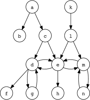
(a) What are the “good moves”, e.g., in position e? Is e won (or lost, or drawn), and if so how?

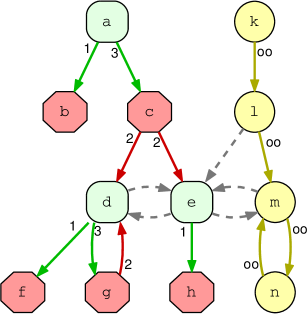
(b) The solved game reveals the answer: move $\mathtt{e}{\to}\mathtt{h}$ is winning; the moves $\mathtt{e}{\to}\mathtt{d}$ and $\mathtt{e}{\to}\mathtt{m}$ are not.

Figure 1: Position values in $G$ (left) are revealed by the solved game $G^{\gamma}=(V,M,\gamma)$ on the right: positions are won (green boxes), lost (red octagons), or drawn (yellow circles). This separates “good” moves (solid, colored arcs) from “bad” ones (dashed, gray). The length $\ell$ of a move $x{\stackrel{{\scriptstyle\ell}}{{\to}}}y$ indicates how quickly one can force a win, or how long one can delay a loss, using that move.

Example. Consider $G=(V,M)$ in Fig. 1a and a start position for player $\mathrm{I}$, say $\mathtt{e}$. In the play $\pi_{1}{=}~{}\mathtt{e}\stackrel{{\scriptstyle\mathrm{I}}}{{\to}}\mathtt{d}\stackrel{{\scriptstyle\mathrm{II}}}{{\to}}\mathtt{f}$, $\mathrm{I}$ cannot move, so $\pi_{1}$ is lost (for $\mathrm{I}$). However, in $\pi_{2}{=}~{}\mathtt{e}\stackrel{{\scriptstyle\mathrm{I}}}{{\to}}\mathtt{h}$, $\mathrm{II}$ cannot move, so $\pi_{2}$ is won (for $\mathrm{I}$). So from position $\mathtt{e}$, the best move is $\mathtt{e}{\to}\mathtt{h}$; the other moves are “bad”: $\mathtt{e}{\to}\mathtt{d}$ loses (see $\pi_{1}$), while $\mathtt{e}{\to}\mathtt{m}$ only draws (if $\mathrm{II}$ sticks to $\mathtt{m}{\to}\mathtt{n}$).

The Value of a Position: Playing Optimally. To determine the true value of $v\in V$, we are not interested in plays with bad moves, but consider instead plays where the opponents play optimally, or at least “good enough” so that the best possible outcome is guaranteed. Hence we ask: can $\mathrm{I}$ force a win from $v\in V$ (no matter what $\mathrm{II}$ does), or can $\mathrm{II}$ force $\mathrm{I}$ to lose from $v$? If neither player can force a win, $v$ is a draw and both players can avoid losing by forcing an infinite play. This is formalized using strategies.

A (pure) strategy is a partial function $S:V\to V$ with $S\subseteq M$. It prescribes which of the available moves a player will choose in a position $v$. We define $v_{0}$ to be won for player $\mathrm{I}$ in (at most) $n$ moves, if there is a strategy $S_{\mathrm{I}}$ for $\mathrm{I}$, such that for all strategies $S_{\mathrm{II}}$ of $\mathrm{II}$, there is a number $j=2k+1\leq n$ such that $v_{j}=S_{\mathrm{I}}\circ(S_{\mathrm{II}}\circ S_{\mathrm{I}})^{k}(v_{0})$ is defined, but $S_{\mathrm{II}}(v_{j})$ is not: $\mathrm{II}$ cannot move. In this case, $S_{\mathrm{I}}$ is a winning strategy for $\mathrm{I}$ at $v_{0}$. Conversely, $v_{0}$ is won for player $\mathrm{II}$ in (at most) $n$ moves, if there is a strategy $S_{\mathrm{II}}$, such that for all strategies $S_{\mathrm{I}}$, there is a number $j=2k\leq n$ such that $v_{j}=(S_{\mathrm{II}}\circ S_{\mathrm{I}})^{k}(v_{0})$ is defined, but $S_{\mathrm{I}}(v_{j})$ is not: $\mathrm{I}$ cannot move. With this, we say the value of $v_{0}$ is won (lost) if it is won for player $\mathrm{I}$ (player $\mathrm{II}$). If $v_{0}$ is neither won nor lost, its value is drawn, so neither $\mathrm{I}$ nor $\mathrm{II}$ can force a win from $v_{0}$, but both can avoid losing via an infinite play.

2.1 Solving Games: Labeling Nodes (Positions)

Let $G=(V,M)$ be the game in Figure 1a. How can we solve $G$, i.e., determine whether the value of $x\in V$ is won, lost, or drawn? We represent the value of $x$ using a node labeling $\gamma:V\to\{{{\color[rgb]{0,0.45,0}\mathsf{W}}},{{\color[rgb]{0.8,0,0}\mathsf{L}}},{{\color[rgb]{0.6,0.6,0}\mathsf{D}}}\}$ and write $G^{\gamma}=(V,M,\gamma)$ to denote a solved game.

The following Datalog^¬ query, consisting of a single rule, solves games:

$$\mathtt{win}(X)\;\mathtt{{:}-}\;\mathtt{move}(X,Y),\neg\mathtt{win}(Y) Q_{G}$$ ()

$Q_{G}$ says that position $x$ is won in $G$ if there is a move to position $y$, where $y$ is not won. For non-stratified Datalog^¬ programs like $Q_{G}$ (having recursion through negation), the three-valued well-founded model $\mathcal{W}$ [24] provides the desired answer:

Proposition 1 ($Q_{G}$ Solves Games)

Let $P\mathbin{{:}{=}}(Q_{G}\cup\mathtt{move})$ be the Datalog^¬ query $Q_{G}$ plus finitely many “$\mathtt{move}$” facts, representing a game $G=(V,M)$. For all $x\in V$:

$$\mathcal{W}_{P}(\,\mathtt{win}(x)\,)=\left\{\begin{array}[]{@{}c@{}}\mathsf{true}{}\\ \mathsf{false}{}\\ \mathsf{undef}{}\end{array}\right\}~{}~{}\Leftrightarrow~{}~{}\gamma(x)=\left\{\begin{array}[]{@{}c@{}}{\color[rgb]{0,0.45,0}{\emph{{{${\color[rgb]{0,0.45,0}\mathsf{W}}$}}}}}\\ {\color[rgb]{0.8,0,0}{\textbf{\emph{{${\color[rgb]{0.8,0,0}\mathsf{L}}$}}}}}\\ {\color[rgb]{0.6,0.6,0}{\emph{{{${\color[rgb]{0.6,0.6,0}\mathsf{D}}$}}}}}\end{array}\right\}~{}.$$

_□

When implemented via an alternating fixpoint [23], one obtains an increasing sequence of underestimates $U_{1}\subseteq U_{2}\subseteq\dots$ converging to the true atoms $U^{\omega}$ from below, and a decreasing sequence of overestimates $O_{1}\supseteq O_{2}\supseteq\dots$ converging to $O^{\omega}$, the union of true or undefined atoms from above. Any remaining atoms in the “gap” have the third truth-value ($\mathsf{undef}$). For the game query $Q_{G}$ above, $U^{\omega}$ contains the won positions $V^{{\color[rgb]{0,0.45,0}\mathsf{W}}}$; the “gap” (if any) $O^{\omega}\setminus U^{\omega}$ contains the drawn positions $V^{{\color[rgb]{0.6,0.6,0}\mathsf{D}}}$; and the atoms in the complement of $O^{\omega}$ (i.e., which are neither true nor undefined) are the lost positions $V^{{\color[rgb]{0.8,0,0}\mathsf{L}}}$.

To solve $G$ directly, consider, e.g., the three moves $\mathtt{e}{\to}\mathtt{d}$, $\mathtt{e}{\to}\mathtt{h}$, and $\mathtt{e}{\to}\mathtt{m}$ in Fig. 1a. The move $\mathtt{e}{\to}\mathtt{h}$ is clearly winning, as it forces the opponent into a sink. However, the status of the moves $\mathtt{e}{\to}\mathtt{d}$ and $\mathtt{e}{\to}\mathtt{m}$ is unclear unless the game has been solved. Fig. 1b depicts the solved game $G^{\gamma}$. The set of positions is a disjoint union $V=V^{{\color[rgb]{0,0.45,0}\mathsf{W}}}\mathbin{\dot{\cup}}V^{{\color[rgb]{0.8,0,0}\mathsf{L}}}\mathbin{\dot{\cup}}V^{{\color[rgb]{0.6,0.6,0}\mathsf{D}}}$.

To obtain $G^{\gamma}$, proceed as follows: First, find all sinks $x$, i.e., nodes for which the set of followers $\mathsf{F}(x)=\{y\mid(x,y)\in M\}$ is empty. These positions are immediately lost and colored red: $V^{{\color[rgb]{0.8,0,0}\mathsf{L}}}_{0}=\{x\in V\mid\mathsf{F}(x)=\emptyset\}$. In our example, $V^{{\color[rgb]{0.8,0,0}\mathsf{L}}}_{0}=\{\mathtt{b},\mathtt{f},\mathtt{h}\}$. We then find all nodes $x$ for which there is some $y$ with $(x,y)\in M$ such that $y\in V^{{\color[rgb]{0.8,0,0}\mathsf{L}}}_{0}$. These positions are won and colored green; here: $V^{{\color[rgb]{0,0.45,0}\mathsf{W}}}_{1}=\{\mathtt{a},\mathtt{d},\mathtt{e}\}$. We then find the unlabeled nodes $x$ for which all followers $y\in\mathsf{F}(x)$ are already won (i.e., colored green). Since the player moving from that position can only move to a position that is won for the opponent, those $x$ are also lost and added to $V^{{\color[rgb]{0.8,0,0}\mathsf{L}}}_{2}$. In our example $V^{{\color[rgb]{0.8,0,0}\mathsf{L}}}_{2}=\{\mathtt{c},\mathtt{g}\}$. We now iterate the above steps until there is no more change. One can show that $V_{1}^{{\color[rgb]{0,0.45,0}\mathsf{W}}}\subseteq V_{3}^{{\color[rgb]{0,0.45,0}\mathsf{W}}}\subseteq V_{5}^{{\color[rgb]{0,0.45,0}\mathsf{W}}}\cdots$ converges to the won positions $V^{{\color[rgb]{0,0.45,0}\mathsf{W}}}$, whereas $V_{0}^{{\color[rgb]{0.8,0,0}\mathsf{L}}}\subseteq V_{2}^{{\color[rgb]{0.8,0,0}\mathsf{L}}}\subseteq V_{4}^{{\color[rgb]{0.8,0,0}\mathsf{L}}}\cdots$ converges to the lost positions $V^{{\color[rgb]{0.8,0,0}\mathsf{L}}}$; the drawn positions are $V^{{\color[rgb]{0.6,0.6,0}\mathsf{D}}}\mathbin{{:}{=}}V\setminus(V^{{\color[rgb]{0,0.45,0}\mathsf{W}}}\cup V^{{\color[rgb]{0.8,0,0}\mathsf{L}}})$.

$V^{{\color[rgb]{0,0.45,0}\mathsf{W}}}\mathbin{{:}{=}}\emptyset$ ;

  // Initially we don’t know any won positions

$V^{{\color[rgb]{0.8,0,0}\mathsf{L}}}\mathbin{{:}{=}}\{x\in V\mid\mathsf{F}(x)=\emptyset\}$ ;

  // $\dots$ but all sinks are lost $\dots$

$\mathrm{len}(x)\mathbin{{:}{=}}0$ for all $x\in V^{{\color[rgb]{0.8,0,0}\mathsf{L}}}$ ;

  // $\dots$ immediately: their length is 0.

repeat

       for $x\in V\setminus(V^{{\color[rgb]{0,0.45,0}\mathsf{W}}}\cup V^{{\color[rgb]{0.8,0,0}\mathsf{L}}}$)  do

             $F^{{\color[rgb]{0.8,0,0}\mathsf{L}}}\mathbin{{:}{=}}\mathsf{F}(x)\cap V^{{\color[rgb]{0.8,0,0}\mathsf{L}}}$;    $F^{{\color[rgb]{0,0.45,0}\mathsf{W}}}\mathbin{{:}{=}}\mathsf{F}(x)\cap V^{{\color[rgb]{0,0.45,0}\mathsf{W}}}$ ;

             if $F^{{\color[rgb]{0.8,0,0}\mathsf{L}}}\neq\emptyset$ then

                  $V^{{\color[rgb]{0,0.45,0}\mathsf{W}}}\mathbin{{:}{=}}V^{{\color[rgb]{0,0.45,0}\mathsf{W}}}\cup\{x\}$ ;

                    // some $y\in\mathsf{F}(x)$ is lost, so $x$ is won

                   $\mathrm{len}(x)\mathbin{{:}{=}}1+\min\{\mathrm{len}(y)\mid y\in F^{{\color[rgb]{0.8,0,0}\mathsf{L}}}\}$ ;

                    // shortest win

                  

            if $\mathsf{F}(x)=F^{{\color[rgb]{0,0.45,0}\mathsf{W}}}$ then

                  $V^{{\color[rgb]{0.8,0,0}\mathsf{L}}}\mathbin{{:}{=}}V^{{\color[rgb]{0.8,0,0}\mathsf{L}}}\cup\{x\}$ ;

                    // all $y\in\mathsf{F}(x)$ are won, so $x$ is lost

                   $\mathrm{len}(x)\mathbin{{:}{=}}1+\max\{\mathrm{len}(y)\mid y\in F^{{\color[rgb]{0,0.45,0}\mathsf{W}}}\}$ ;

                    // longest delay

                  

            

      

until $V^{{\color[rgb]{0,0.45,0}\mathsf{W}}}$ and $V^{{\color[rgb]{0.8,0,0}\mathsf{L}}}$ change no more;

$V^{{\color[rgb]{0.6,0.6,0}\mathsf{D}}}\mathbin{{:}{=}}V\setminus(V^{{\color[rgb]{0,0.45,0}\mathsf{W}}}\cup V^{{\color[rgb]{0.8,0,0}\mathsf{L}}})$ ;

  // remaining positions are now draws

$\mathrm{len}(x)\mathbin{{:}{=}}\infty$ for all $x\in V^{{\color[rgb]{0.6,0.6,0}\mathsf{D}}}$ ;

  // $\dots$ and can be delayed forever

$\gamma(x)\mathbin{{:}{=}}{{\color[rgb]{0,0.45,0}\mathsf{W}}}/{{\color[rgb]{0.8,0,0}\mathsf{L}}}/{{\color[rgb]{0.6,0.6,0}\mathsf{D}}}$ for all $x\in V^{{\color[rgb]{0,0.45,0}\mathsf{W}}}/V^{{\color[rgb]{0.8,0,0}\mathsf{L}}}/V^{{\color[rgb]{0.6,0.6,0}\mathsf{D}}}$, respectively.

Algorithm 1 Solve game $G^{\gamma}=(V,M,\gamma)$

Algorithm 1 depicts the details of a simple, round-based approach to solve games. In it, we also compute the length of a position, which adds further information to a solved game $G^{\gamma}$, i.e., how quickly one can win (starting from green nodes), or how long one can delay losing (starting from red nodes). In Fig. 1, the (delay) length of $\mathtt{f}$ is 0, since $\mathtt{f}$ is a sink and no move is possible. In contrast, the (win) length of $\mathtt{d}$ is 1: the next player moving wins by moving to $\mathtt{f}$. For $\mathtt{g}$, the (delay) length is 2, since the player can move to $\mathtt{d}$, but the opponent can then move to $\mathtt{f}$. So $\mathtt{g}$ is lost in 2 moves.

Remark. As described, Algorithm 1 proceeds in rounds to determine the value of positions, i.e., in each round $i$, all newly won positions, and all newly lost positions are determined. This could be used, e.g., to simplify the computation of the length of a position ($\mathrm{len}(x)$ can be derived from the first round in which the value of $x$ becomes known). On the other hand, this is not strictly necessary: one can replace the for-loop ranging over all unlabeled nodes by a non-deterministic pick of any unlabeled node. As long as we pick nodes in a fair manner, the non-deterministic version will also converge to the correct result, while allowing more flexibility during evaluation [26].

2.2 Game Provenance: Labeling Edges (Moves)

	$y$ won (${\color[rgb]{0,0.45,0}\mathsf{W}}$)	$y$ drawn (${\color[rgb]{0.6,0.6,0}\mathsf{D}}$)	$y$ lost (${\color[rgb]{0.8,0,0}\mathsf{L}}$)
$x$ won (${\color[rgb]{0,0.45,0}\mathsf{W}}$)	bad	bad	${\color[rgb]{0,0.45,0}\mathsf{g}}$: winning
$x$ drawn (${\color[rgb]{0.6,0.6,0}\mathsf{D}}$)	bad	${\color[rgb]{0.6,0.6,0}\mathsf{y}}$: drawing	n/a
$x$ lost (${\color[rgb]{0.8,0,0}\mathsf{L}}$)	${\color[rgb]{0.8,0,0}\mathsf{r}}$: delaying	n/a	n/a

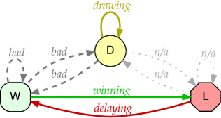
Figure 2: Depending on node labels, moves $x\to y$ are either winning (or green) (${{\color[rgb]{0,0.45,0}\mathsf{W}}}\stackrel{{\scriptstyle{{\color[rgb]{0,0.45,0}\mathsf{g}}}}}{{\leadsto}}{{\color[rgb]{0.8,0,0}\mathsf{L}}}$), delaying (or red) (${{\color[rgb]{0.8,0,0}\mathsf{L}}}\stackrel{{\scriptstyle{{\color[rgb]{0.8,0,0}\mathsf{r}}}}}{{\leadsto}}{{\color[rgb]{0,0.45,0}\mathsf{W}}}$), or drawing (or yellow) (${{\color[rgb]{0.6,0.6,0}\mathsf{D}}}\stackrel{{\scriptstyle{{\color[rgb]{0.6,0.6,0}\mathsf{y}}}}}{{\leadsto}}{{\color[rgb]{0.6,0.6,0}\mathsf{D}}}$). All other moves are either bad (allowing the opponent to improve the outcome), or non-existent (n/a): e.g., if $x$ is lost, then there are only delaying moves (i.e., ending in won positions $y$ for the opponent).

We return to our original question: why is $x\in V$ won, lost, or drawn? We would like to define a suitable notion of game provenance $\mathrm{\Gamma}(x)$ that is similar in spirit to the how-provenance devised for positive queries [15], but that works for games and explains the value (won, lost, or drawn) of $x$. Some desiderata of game provenance are immediate: First, only nodes reachable from $x$ can influence the outcome at $x$, i.e., only nodes and edges in the transitive closure $\mathsf{F}^{+}(x)$. Thus, one expects $\mathrm{\Gamma}(x)$ to depend only on $\mathsf{F}^{+}(x)$. In addition, one expects the value $\gamma(x)$ of position $x$ to be independent of “bad moves”, i.e., which give the opponent a better outcome than necessary. We use a partial edge-labeling function $\lambda$ to distinguish different types of moves.

Definition 1 (Edge Labels)

Let $G^{\gamma}=(V,M,\gamma)$ be a solved game. The edge-labeling $\lambda:V\times V\to\{{{\color[rgb]{0,0.45,0}\mathsf{g}}},{{\color[rgb]{0.8,0,0}\mathsf{r}}},{{\color[rgb]{0.6,0.6,0}\mathsf{y}}}\}$ defines a color for a subset of edges from $M$ as shown in Fig. 2. _□

In Figure 2 we use $\gamma(x)$ and $\gamma(y)$, i.e., node labels ${\color[rgb]{0,0.45,0}\mathsf{W}}$, ${\color[rgb]{0.6,0.6,0}\mathsf{D}}$, and ${\color[rgb]{0.8,0,0}\mathsf{L}}$ of moves $(x,y)\in M$ to derive an appropriate edge label. This allows us to distinguish provenance-relevant (“good”) moves (winning, drawing, or delaying), from irrelevant (bad) moves. The latter are excluded from game provenance:

Definition 2 (Game Provenance)

Let $G^{\gamma}=(V,M,\gamma)$ be a solved game. The game provenance $\mathrm{\Gamma}({=}\mathrm{\Gamma}_{G})$ is the $\lambda$-colored subgraph of $G^{\gamma}$. For $x\in V$, we define $\mathrm{\Gamma}(x)$ as the subgraph of $\mathrm{\Gamma}$, reachable via $\lambda$ edges. _□

Consider the solved game on the right in Fig. 1. Since bad (dashed) edges are excluded, the game provenance consists of two disconnected subgraphs: (i) The bipartite “red-green” subgraph, which is draw-free, i.e., every position is either won or lost, and (ii) the “yellow” subgraph, representing the drawn positions.

The figure also reveals that solved games $G^{\gamma}$ and thus game provenance $\mathrm{\Gamma}$ have a nice, regular structure. The following is immediate from the underlying game-theoretic semantics of $G$.

Theorem 1 (Provenance Structure)

Let $G^{\gamma}=(G,M,\gamma)$ be a solved game, $\mathrm{\Gamma}$ its edge-labeled provenance graph. The game provenance $\mathrm{\Gamma}$ has a regular structure:

$$\mathrm{\Gamma}(x)=\left\{\begin{array}[]{ll}M_{{{\color[rgb]{0,0.45,0}\mathsf{g}}}.({{\color[rgb]{0.8,0,0}\mathsf{r}}}.{{\color[rgb]{0,0.45,0}\mathsf{g}}})^{*}}(x)&\mbox{; if $x$ is won}\\ M_{({{\color[rgb]{0.8,0,0}\mathsf{r}}}.{{\color[rgb]{0,0.45,0}\mathsf{g}}})^{*}}(x)&\mbox{; if $x$ is lost}\\ M_{{{\color[rgb]{0.6,0.6,0}\mathsf{y}}}^{+}}(x)&\mbox{; if $x$ is drawn}\end{array}\right.$$

_□

Here, for a regular expression $R$, and a node $x\in V$, the expression $M_{R}(x)$ denotes a subset of labeled edges of $M$, i.e., for which there is a path $\pi$ in $\mathrm{\Gamma}$ whose labels match the expression $R$. As we shall see below, for positive queries, the bipartite structure of won and lost nodes nicely corresponds to the structure of provenance polynomials [19].

3 Provenance Games

The game semantics (avoiding bad moves) yields a natural model of provenance. We now apply this notion to queries expressed using non-recursive Datalog^¬ rules. Any first-order query $\varphi(\bar{x})$ on input database $D$ can be expressed as a non-recursive Datalog^¬ program $Q_{\varphi}$ with a distinguished relation $\mathtt{ans}\in\textit{idb}(Q_{\varphi})$ such that evaluating $Q_{\varphi}$ with input $D$ under the stratified semantics agrees with the result of $\varphi(\bar{x})$. In the following we use $Q(D)$ to denote the result of evaluating $Q$ on input $D$.

3.1 Query Evaluation Games

Move	Claim made by making the move
$\mathsf{A}\stackrel{{\scriptstyle\exists}}{{\leadsto}}\mathsf{R}$	“$A$ is true: it’s the head of this instance of ${R}$.”
$\mathsf{R}\leadsto\mathsf{G}$	“Positive goal $g_{k}({=}A^{\prime})$ in your rule body fails!”
$\mathsf{G}\leadsto\neg\mathsf{A}$	“No! Its negation $\neg A^{\prime}$ fails and $A^{\prime}$ is true.”
$\neg\mathsf{A}\leadsto\mathsf{A}$	“No: atom $A^{\prime}$ fails!”
$\mathsf{R}\leadsto\mathsf{N}$	“Negative goal $\neg A^{\prime}$ in the rule body fails.”
$\mathsf{N}\leadsto\mathsf{A}$	“No: $\neg A^{\prime}$ succeeds, but $A^{\prime}$ fails.”

Figure 3: Move types of the query evaluation game (left) and implicit claims made (right). Moving along an edge, a player aims to verify a claim, thereby refuting the opponent. Initially, player $\mathrm{I}$ is a verifier, trying to prove $A$, while $\mathrm{II}$ tries to spoil this attempt and refute it. Roles are swapped ($\mathrm{I}$ $\rightleftharpoons$ $\mathrm{II}$) when moving through a negated goal ($\mathsf{R}{\leadsto}\mathsf{N}{\leadsto}\mathsf{A}$).

Query evaluation of $Q(D)$ can be seen as a game between players $\mathrm{I}$ and $\mathrm{II}$ who argue whether an atom $A\in Q(D)$. The argumentation structure is stylized in Fig. 3. There are three classes of positions in the game as shown on the left of Figure 3:

• Relation nodes—depicted as circles,

• Rule nodes—depicted as rectangles, and

• Goal nodes—depicted as rectangles with rounded corners.

Both relation nodes and goal nodes can be positive or negative.

Usually, an evaluation game starts with I claiming that a ground atom $A(x)$ is true. That is she starts the game in a relation node for $A$. To substantiate her claim she moves to a rule that has $A$ as a head atom and specifies constants for the remaining existentially quantified variables in the body of the rule. Now, II tries to reject the validity of the rule by selecting a goal atom (e.g., $B$) in its body that he thinks is not satisfied (e.g., II moves to the goal node for $B$). I then moves to a negated relation node for this goal (eg, a node $\neg B$), claiming the goal is true because its negation is false. From here, II moves to the relation node $B$, questioning I’s claim that $B$ is true. The game then continues in the same way. Note that the graph on the left of in Fig. 3 is a schema-level description. When one cycle (relation$\leadsto$rule$\leadsto$goal$\leadsto$$\neg$relation$\leadsto$relation) is complete, the actual fact that is argued about has changed (e.g., from $A$ to $B$). If II selects a negated goal (e.g., $\neg C$) in the body of a rule then player I moves directly from the negated goal node to the relation node for $C$. This essentially switches the roles of I and II since now player II has to argue for a relation node $C$.

(a) ${Q_{\mathtt{neg}}}$ as a game diagram

$$\begin{array}[]{lcl}\textnormal{{Atoms} $A$,$B$, {and} $C$}\\ \mathtt{M}(f_{\mathtt{\neg{}A}}(X),f_{\mathtt{A}}(X))&\;\mathtt{{:}-}&\mathtt{d}(X).\\ \mathtt{M}(f_{\mathtt{\neg{}B}}(X,Y),f_{\mathtt{B}}(X,Y))&\;\mathtt{{:}-}&\mathtt{d}(X),\mathtt{d}(Y).\\ \mathtt{M}(f_{\mathtt{\neg{}C}}(X),f_{\mathtt{C}}(X))&\;\mathtt{{:}-}&\mathtt{d}(X).\\ \\ \textnormal{{IDB} $A$ {via rule} $r_{1}$}\\ \mathtt{M}(f_{\mathtt{A}}(X),f_{\mathtt{r_{1}}}(X,Y))&\;\mathtt{{:}-}&\mathtt{d}(X),\mathtt{d}(Y).\\ \mathtt{M}(f_{\mathtt{r_{1}}}(X,Y),f_{\mathtt{g_{1}^{1}}}(X,Y))&\;\mathtt{{:}-}&\mathtt{d}(X),\mathtt{d}(Y).\\ \mathtt{M}(f_{\mathtt{r_{1}}}(X,Y),f_{\mathtt{g_{1}^{2}}}(Y))&\;\mathtt{{:}-}&\mathtt{d}(X),\mathtt{d}(Y).\\ \mathtt{M}(f_{\mathtt{g_{1}^{1}}}(X,Y),f_{\mathtt{\neg{}B}}(X,Y))&\;\mathtt{{:}-}&\mathtt{d}(X),\mathtt{d}(Y).\\ \mathtt{M}(f_{\mathtt{g_{1}^{2}}}(X),f_{\mathtt{C}}(X))&\;\mathtt{{:}-}&\mathtt{d}(X).\\ \\ \textnormal{{EDB} $B$ {and} $C$}\\ \mathtt{M}(f_{\mathtt{B}}(X,Y),f_{\mathtt{r_{B}}}(X,Y))&\;\mathtt{{:}-}&\mathtt{B}(X,Y).\\ \mathtt{M}(f_{\mathtt{C}}(X),f_{\mathtt{r_{C}}}(X))&\;\mathtt{{:}-}&\mathtt{C}(X).\end{array}$$

(b) Rules defining the moves for ${Q_{\mathtt{neg}}}$

(c) Instantiated game $G_{Q_{\mathtt{neg}},D}$ for $D=\{B(a,b),B(b,a),C(a)\}$

(d) Solved game $G^{\gamma}_{Q_{\mathtt{neg}},D}$. Lost positions are (dark) red; won positions are (light) green. Provenance edges (good moves) are solid; bad moves are dashed. $A(a)$ (resp. $A(b)$) is true (resp. false), indicated by position value ${\color[rgb]{0,0.45,0}\mathsf{W}}$ (resp. ${\color[rgb]{0.8,0,0}\mathsf{L}}$). The game provenance $\mathrm{\Gamma}(A(a))$ explains why/how $A(a)$ is true; $\mathrm{\Gamma}(A(b))$ explains why-not $A(b)$.

Figure 4: Provenance game for the FO query ${Q_{\mathtt{neg}}}{\mathbin{{:}{=}}}~{}{\mathtt{A}(X)\;\mathtt{{:}-}\;\mathtt{B}(X,Y),\neg\mathtt{C}(Y).}$ The well-founded model of the rule $\mathtt{win}(X)\;\mathtt{{:}-}\;\mathtt{M}(X,Y),\neg\mathtt{win}(Y)$, applied to the move graph $\mathtt{M}$, solves the game.

We now demonstrate the general argumentation scheme for a concrete Datalog^¬ program ${Q_{\mathtt{neg}}}$. The program ${Q_{\mathtt{neg}}}$ consists of a single rule $r_{1}$:

$$r_{1}:\quad\mathtt{A}(X)\;\mathtt{{:}-}\;\underbrace{\mathtt{B}(X,Y)}_{\mathnormal{g_{1}}},\;\underbrace{\neg\,\mathtt{C}(Y)}_{\mathnormal{g_{2}}} {Q_{\mathtt{neg}}}$$ ()

The game diagram for ${Q_{\mathtt{neg}}}$ is shown in Fig. 4a. Player $\mathrm{I}$ starts in a relation node of type $A(X)$ with a concrete instatiation $X=x$ to prove that $\mathtt{A}(x)\in Q(D)$. In her first move, she picks the rule $r_{1}$ together with bindings for all existentially quantified variables in $r_{1}$, which is just a instatiation $y$ for $Y$ in $r_{1}$; essentially picking a ground instance $r_{1}(x,y)$ such that the variable $X$ is bound to the desired $x$. She claims the rule body is satisfied. If this is not the case, $\mathrm{II}$ can falsify the claim by selecting a goal from the body, i.e., either $g_{1}^{1}(x,y)$, thus making a counter-claim that $\mathtt{B}(x,y)$ is false, or $g_{1}^{2}(y)$, claiming instead that $C(y)$ is true. Positive case, e.g., $\mathrm{II}$ moved to $g_{1}^{1}(x,y)$. Player $\mathrm{I}$ will move from $g_{1}^{1}(x,y)$ to $\neg B(x,y)$, from which $\mathrm{II}$ will move to $B(x,y)$. In this node, there is an edge for player $\mathrm{I}$ if and only if $B(x,y)\in D$, that is if there is a trivial, bodyless rule $r_{B}(x,y)$ representing this fact. Thus, $\mathrm{I}$ wins the game if $B(x,y)\in D$ and $\mathrm{II}$ wins if $B(x,y)\not\in D$. Negative case, e.g., $\mathrm{II}$ just moved to $g_{1}^{2}(y)$. Player $\mathrm{I}$ moves to the instatiation $\mathtt{C}(y)$ of relation node $C(X)$. For this move in the diagram, variables used in the goal node are explicitely renamed to the single variable name used in the corresponding relation node. With this move, $\mathrm{II}$ loses and $\mathrm{I}$ wins if $C(y)\not\in D$; $\mathrm{II}$ wins the argument if $C(y)\in D$ by moving to the trivial rule node, forcing $\mathrm{I}$ to lose.

Construction of Evaluation Game Graph. We create a game in which the constants are also encoded within the game positions. In Fig. 4b, we provide Datalog rules that define the move relation $\mathtt{M}$ of the evaluation game $G_{{Q_{\mathtt{neg}}},D}$ for ${Q_{\mathtt{neg}}}$ with an input database $D$. Here, $\mathtt{d}$ is a relation that contains the active domain of ${Q_{\mathtt{neg}}}$ and $D$.

For each ground atom, we create a postive and a negative relation node. We use Skolem functions to create “node identifiers”. E.g., for a ground atom $\mathtt{S(a_{1},\dots,a_{n})}$ we use $f_{S}(\mathtt{a_{1},\dots,a_{n}})$ for its positive relation nodes and $f_{\neg{}S}(\mathtt{a_{1},\dots,a_{n}})$ for its negative relation node. The first three rules in Fig. 4b create an edge from the negative to the positive node.

Furthermore, we create a rule node for each rule $r_{i}$ in the ground program with a unique identifier $f_{r_{i}}(X_{1},\dots,X_{n})$ including the rule number and the assignments of variables found in the rule’s body to constants. For simplicity, we alphabetically order variables and provide the constants in this order. There is an edge from the ground head atom to the ground rule node (cf. Fig. 4b first line of middle block). For example, the Skolem function $f_{r_{1}}(a,b)$ encodes the whole rule body $r1:[B(a,b),\neg{}C(b)]$.

Then, we add moves from rule node $r_{i}$ to its goal nodes $g_{i}^{j}$. Goal nodes are identified by the rule number $i$ they occur in, their positions $j$ within the body, and the bound constants. (cf. lines 2 and 3 of middle block). From positive (negative) goal nodes, we move to negative (positive) relation nodes keeping the bound constants fixed (cf. lines 4 and 5 of middle block). Finally, for edb relations, we add an edge from the positive relation node $R(\bar{c})$ to a rule node $f_{\mathtt{r_{R}}}(\bar{c})$ iff $R(\bar{c})\in D$. This ensures that a player reaching the relation node $R(\bar{c})$ wins iff $R(\bar{c})\in D$. In Fig. 4c the game graph for ${Q_{\mathtt{neg}}}$ with input database $D=\{B(a,b),B(b,a),C(a)\}$ is shown. The solved game is shown in Fig. 4d. Here, we see that $\mathrm{I}$ has a winning strategy for e.g., $A(a)$, $B(b,a)$, and $C(a)$.

Acyclicity of FO Games. For FO queries, represented by non-recursive Datalog^¬ programs, no relation node is reachable from itself and the resulting game graph is acyclic.

Theorem 2 (FO Provenance Game)

Consider a first-order query $\varphi$ in the form of a non-recursive Datalog^¬ program ${Q_{\varphi}}$ with output relation $\mathtt{ans}$ and input database facts $D$. Let $G^{\gamma}_{Q_{\varphi},D}=(V,M,\gamma)$ be the solved game. Then:

1. $G^{\gamma}_{Q_{\varphi},D}$ is draw-free.

2. ${Q_{\varphi}}(\,\mathtt{ans}(\bar{x})\,)=\left\{\begin{array}[]{@{}c@{}}\mathsf{true}{}\\ \mathsf{false}{}\\ \end{array}\right\}\Leftrightarrow\gamma(\,f_{\mathtt{ans}}(\bar{x})\,)=\left\{\begin{array}[]{@{}c@{}}{\color[rgb]{0,0.45,0}{\emph{{{${\color[rgb]{0,0.45,0}\mathsf{W}}$}}}}}\\ {\color[rgb]{0.8,0,0}{\textbf{\emph{{${\color[rgb]{0.8,0,0}\mathsf{L}}$}}}}}\\ \end{array}\right\}$

Sketch. It is easy to see that one can associate with every non-recursive Datalog^¬ program $Q$ and input $D$ an evaluation game graph $G_{Q,D}$ together with a solved game $G^{\gamma}_{Q,D}$. Since the game graph is acyclic, the solved game will not contain any drawn positions. Further, by construction, $G^{\gamma}_{Q,D}$ models query evaluation of $Q(D)$. _□

3.2 Relationship with Provenance Polynomials – How-Provenance for $\mathcal{RA}^{+}$

Game graphs are constructed to preserve provenance information available in program and database. It turns out that for positive Datalog programs $Q$ they generate semiring provenance polynomials as defined in [15, 19] for atoms $A(\bar{x})\in Q(D)$.

Semiring Provenance Polynomials. Semiring provenance [15, 19] attaches provenance information to EDB and IDB facts. The provenance information are elements of a commutative semiring $K$. A commutative semiring is an algebraic structure with two distinct associative and commutative operations “$+$” and “$\times$”. During query evaluation, result facts are annotated with elements from $K$ that are created by combining the provenance information from input facts. For example, in the join $\mathtt{R(a,b)\;\mathtt{{:}-}\;S(a,b),T(a)}$ with $\mathtt{S(a,b)}$ being annotated with $p_{1}\in K$ and $\mathtt{T(a)}$ being annotated with $p_{2}\in K$, the result fact $\mathtt{R(a,b)}$ will be annotated with $p_{1}\times p_{2}$. Intuitively, “$\times$” is used to combine provenance information of joint use of input facts, whereas “$+$” is used for alternative use of input facts.

Depending on the conrete semiring used, different (provenance) information is propagated during query evaluation. The most informative semiring is the positive algebra provenance semiring ${\mathbb{N}[X]}$ [15, 19] whose elements are polynomials with variables from a set $X$ and coefficients from $\mathbb{N}$. The operators “$\times$” and “$+$” in ${\mathbb{N}[X]}$ are the usual addition and multiplication of polynomials. Usually, facts from the input database $D$ are annotate by variables from a set $X$. Formally, we use $\mathcal{P}^{{\mathbb{N}[X]}}$ as a function that maps a ground atom to its provenance annotation in ${\mathbb{N}[X]}$.

Obtaining Semiring Polynomials from Game Provenance. Let $Q$ be a positive query, and fix an atom $A(\bar{x})\in Q(D)$. The provenance graph $\mathrm{\Gamma}_{Q,D}(f_{\mathtt{A}}(\bar{x}))=(V,M,\gamma)$ for $A(\bar{x})$ can easily be transformed into an operator tree for a provenance polynomial. The operator tree is represented as a DAG $G^{\mathrm{\Omega}}(A(\bar{x}))$ in which common sub-expressions are re-used. $G^{\mathrm{\Omega}}(A(\bar{x}))=(V^{\prime},M^{\prime},\delta)$ has nodes $V^{\prime}$, edges $M^{\prime}$, and node labels $\delta$. For a fixed $A(\bar{x})$, the structures of $\mathrm{\Gamma}$ and $G^{\mathrm{\Omega}}$ coincide, that is $V=V^{\prime}$ and $M=M^{\prime}$. The labeling function $\delta$ maps inner nodes to either “$+$” or “$\times$”, denoting n-ary versions of the semiring operators. Leaf nodes in game provenance graphs correspond to atoms over the EDB schema. We here only assign elements from $K$ to leaf nodes of the form $f_{\mathtt{r_{R}}}(\bar{x})$. Formally, the labeling function $\delta$ is defined as follows:

$$\delta(v)=\begin{cases}\mathcal{P}^{{\mathbb{N}[X]}}(A(\bar{x}))&\textnormal{if }\;\;\mathsf{F}(v)=\emptyset\;\textnormal{ and }\;v=f_{\mathtt{r_{A}}}(\bar{x})\\ \mbox{``$\times$''}&\textnormal{if }\;\;\mathsf{F}(v)\neq\emptyset\;\textnormal{ and }\;\gamma(v)={{\color[rgb]{0.8,0,0}\mathsf{L}}}\\ \mbox{``$+$''}&\textnormal{if }\;\;\mathsf{F}(v)\neq\emptyset\;\textnormal{ and }\;\gamma(v)={{\color[rgb]{0,0.45,0}\mathsf{W}}}\\ \end{cases}$$ (1)

We use $\mathrm{\Omega}$ to denote the transformation of obtaining $G^{\mathrm{\Omega}}(A(\bar{x}))$ from $\mathrm{\Gamma}_{Q,D}(f_{\mathtt{A}}(\bar{x}))$. The provenance semiring polynomial of fact $A(\bar{x})$ is now explicit in $G^{\mathrm{\Omega}}(A(\bar{x}))$. An inner node “$+$” (or “$\times$”) with $n$ children represents an $n$-ary version of $+$ (or $\times$) from the semiring. Since the semiring operators are associative and commutative, their $n$-ary versions are well-defined.

Proposition 2

For positive $Q$, and $A(\bar{x})\in Q(D)$, all leaves in $\mathrm{\Gamma}_{Q,D}(A(\bar{x}))$ are of type $f_{\mathtt{r_{B}}}(X,Y)$; thus the labeling described above is complete.

Sketch. For positive programs, positive relation nodes are reachable from other positive relation nodes over a path of length four as shown on the left side of Fig. 3. For an atom $A(\bar{x})\in Q(D)$, all reachable rule nodes are lost and all reachable goal nodes are won. _□

(a) Input database $D$

hop		node $n$	$\delta(n)$
a	a	$f_{\mathtt{r_{hop}}}(a,a)$	$p$
a	b	$f_{\mathtt{r_{hop}}}(a,b)$	$q$
b	a	$f_{\mathtt{r_{hop}}}(b,a)$	$r$
b	c	$f_{\mathtt{r_{hop}}}(b,c)$	$s$

(b) Labels $\delta$ for leaf nodes of $\mathrm{\Gamma}_{Q_{\mathtt{3Hop}},D}$.

3hop		node $n$	$\mathcal{P}^{{\mathbb{N}[X]}}_{Q_{\mathtt{3Hop}},D}(n)$
a	a	$f_{\mathtt{3Hop}}(a,a)$	$p^{3}+2pqr$

(c) ${{\mathbb{N}[X]}}$-Provenance of $f_{\mathtt{3Hop}}(a,a)$.

(d) $\mathrm{\Gamma}(\,f_{\mathtt{3Hop}}(a,a)\,)$

(e) DAG $G^{\mathrm{\Omega}}=\mathrm{\Omega}\circ\mathrm{\Gamma}(f_{\mathtt{3Hop}}(a,a)).\quad\;$ Interpreting $G^{\mathrm{\Omega}}$ yields $p^{3}+2pqr$.

Figure 5: Input graph for program ${Q_{\mathtt{3Hop}}}$ in (a) using edge labeling according to (b). Game provenance $\mathrm{\Gamma}_{Q_{\mathtt{3Hop}},D}$ for the query $\mathtt{3Hop(a,a)}$ on input database of (a) is shown in (d). When labeling leaf nodes according to (b), lost inner nodes by “$\times$”, and won inner nodes by “$+$” then the operator DAG $G^{\mathrm{\Omega}}$ shown in (e) is created. This DAG represents the semiring-provenance polynomial for the query $\mathtt{3Hop(a,a)}$ shown in (c) and [19].

The following theorem relates semiring provenance polynomials to the provenance expressions we obtain in $G^{\mathrm{\Omega}}$:

Theorem 3

Let $\mathrm{\Gamma}_{Q,D}$ be the game provenance of an $\mathcal{RA}^{+}$ query $Q$ (in the form of a positive, non-recursive Datalog program) over database $D$. Then $\mathrm{\Gamma}_{Q,D}$ represents the provenance polynomials ${\mathbb{N}[X]}$ as follows: for all $A(\bar{x})\in Q(D)$,

$$\mathrm{\Omega}\circ\mathrm{\Gamma}_{Q,D}(\,f_{\mathtt{A}}(\bar{x})\,)\equiv\mathcal{P}^{\mathbb{N}[X]}_{Q,D}(\,A(\bar{x})\,).$$

Sketch. Our game graph construction is an extension of the graph presented in Section 4.2 of [19]. Rule nodes correspond to the join nodes presented in [19]. Named goal nodes can be seen as labels on the edges between (goal) tuple nodes and join nodes and allow us to identify at which position a tuple was used in the body. For a detailed proof, please refer to Appendix 0.A. _□

Example $\mathtt{\mathbf{3hop}}$ from [19].   Consider the $\mathtt{3Hop}$ query ${Q_{\mathtt{3Hop}}}$ used in Figure 7 of [19]:

$$r_{1}:\quad\mathtt{3Hop}(X,Y)\,\mathtt{{:}-}\,\mathtt{hop}(X,Z_{1}),\mathtt{hop}(Z_{1},Z_{2}),\mathtt{hop}(Z_{2},Y).$$

The query uses an input database consisting of a single binary EDB relation $\mathtt{hop}$ representing a directed graph. It asks for pairs of nodes that are reachable via exactly three edges(=hops). An input database $D$ and $\mathcal{P}^{{\mathbb{N}[X]}}_{Q_{\mathtt{3Hop}},D}$ annotations of ${Q_{\mathtt{3Hop}}}$ are shown in Fig. 5b. Figure 5d shows the game provenance $\mathrm{\Gamma}(f_{\mathtt{3Hop}}(a,a))$ of fact $\mathtt{3Hop(a,a)}$. Positive won relation nodes indicate the existence of the corresponding fact in ${Q_{3Hop}}(D)$. To obtain the provenance polynomial of fact $f_{\mathtt{3Hop}}(a,a)$, we apply $\mathrm{\Omega}$ to $\mathrm{\Gamma}(f_{\mathtt{3Hop}}(a,a))$ as shown in Fig. 5e: we replace inner won nodes by “$\times$”, inner lost nodes by “$+$”, and leaf nodes by their respective annotations from $K$ as given in Fig. 5b and [19]. The so relabeled graph encodes the provenance equation

$$\mathrm{\Omega}\circ\mathrm{\Gamma}_{Q_{\mathtt{3Hop}},D}(f_{\mathtt{3Hop}}(a,a))=(p\times p\times p)+(p\times q\times r)+(p\times q\times r)=p^{3}+2pqr$$

which is equivalent to the annotation of provenance semiring polynomials as shown in Fig. 5c and [19].

3.3 Why-Not Game Provenance for $\mathcal{RA}^{+}$

Figure 6: Why-not provenance for $\mathtt{3Hop(c,a)}$ using provenance games.

Game provenance also yields meaningful explanations for why-not questions. Consider for example the query ${Q_{\mathtt{3Hop}}}$ and its input database $D$. The atom $\mathtt{3Hop}(c,a)$ is not in ${Q_{\mathtt{3Hop}}}(D)$ and we want to get an explanation why. Figure 6 shows the game provenance $\mathrm{\Gamma}_{Q_{\mathtt{3Hop}},D}(f_{\mathtt{\neg{}3Hop}}(c,a))$ of the missing fact $\mathtt{3Hop(c,a)}$. The lost relation node $\mathtt{3Hop}(c,a)$ indicates that player I will lose the argument that tries to show that $\mathtt{3Hop}(c,a)\in{Q_{3Hop}}(D)$. The game provenance explains why: Any ground instantiation of rule $r_{1}$ will be winning node for player II. Consider, e.g., moving to $r_{1}(c,a,a,a)$ which represents the rule instantiation for $X/{}c,Y/{}a,Z_{1}/{}a,Z_{2}/{}a$. Player II wins the game here by questioning that the first goal $g_{1}^{1}(c,a)$ is satisfied. And indeed, player I will move from $g_{1}^{1}(c,a)$ to $\neg\mathtt{hop}(c,a)$; II to $\mathtt{hop}(c,a)$. Now, I loses the game since $\mathtt{hop}(c,a)\not\in D$ and thus there is no move out of $\mathtt{hop}(c,a)$. We also see that another rule instantiation $X/{}c,Y/{}a,Z_{1}/{}a,Z_{2}/{}b$ fails for the same reason: the missing $\mathtt{hop}(c,a)$. The instantiation $X/{}c,Y/{}a,Z_{1}/{}b,Z_{2}/{}a$ fails because $\mathtt{hop}(c,b)$ is not in the input. Other instantiations, such as $X/{}c,Y/{}a,Z_{1}/{}c,Z_{2}/{}b$, fail because two facts are missing from the input, here $\mathtt{hop}(c,b)$ and $\mathtt{hop}(c,c)$.

It is no coincidence that all leaf nodes represent missing EDB facts for why-not provenance in positive non-recursive Datalog programs:

Proposition 3

Let $Q$ be a non-recursive Datalog program, $D$ a database, $\mathrm{\Gamma}(f_{\mathtt{A}}(\bar{x}))$ the game provenance for facts $A(\bar{x})\not\in Q(D)$. All leaves of $\mathrm{\Gamma}(f_{\mathtt{A}}(\bar{x}))$ have type $f_{\mathtt{R}}(\bar{y})$ and represent ground EDB atoms $R(\bar{y})$ that are missing from the input. _□

The above proposition illustrates that for positive queries, the ultimate reason for failure to derive outputs are missing inputs, represented by the leaves in provenance games.

As defined, game provenance is sensitive to the active domain of query and input database, which can lead to interesting effects. Consider the following query variant $Q^{\prime}_{\mathtt{neg}}\mathbin{{:}{=}}{Q_{\mathtt{neg}}}\cup\{\mathtt{C}(y)\;\mathtt{{:}-}\;\mathtt{E}(y,z)\}$ with input $D=\{\mathtt{B}(a,a)\}$. Here, game provenance shows that $\mathtt{A}(a)$ depends on the presence of $\mathtt{B}(a,a)$ as well as on the absence of $\mathtt{E}(a,a)$. The game provenance graph does not mention that the absence, e.g., of $\mathtt{E}(a,b)$ is important as well—simply because $b$ is not in the active domain.

3.4 Game Provenance for First-Order Queries

In this section, we demonstrate examples for provenance games in the presence of negation within the query. When constructing game graphs for Datalog^¬ queries with negated goals, we obtain graphs in which there exists a path of length three between positive relation nodes. This switches roles between player I and II. In other words, to explain why a negated subgoal is satisfied, an argument like in the why-not case is used. In general, this leads to provenance graphs that contain leaf nodes of both kinds: $f_{\mathtt{C}}(\bar{x})$ representing missing facts $\mathtt{R}(\bar{x})\not\in D$ and $f_{\mathtt{r_{R}}}(\bar{x})$ representing input facts $\mathtt{R}(\bar{x})\in D$.

In the following, we provide examples based on the ${Q_{\mathtt{neg}}}$ query (cf. Fig. 4) with input database $D=\left\{B(a,b),B(b,a),C(a)\right\}$.

(a) Game provenance graph $\mathrm{\Gamma}(f_{\mathtt{A}}(a))$ for $A(a)\in{Q_{\mathtt{neg}}}(D)$.

(b) Game provenance graph $\mathrm{\Gamma}(f_{\mathtt{\neg{}A}}(b))$ for $A(b)\not\in{Q_{\mathtt{neg}}}(D)$

Figure 7: Provenance graphs for ${Q_{\mathtt{neg}}}$ with database $D=\{B(a,b),B(b,a),C(a)\}$. Both why and why-not graphs might contain leaf nodes representing existent and missing input facts.

Why Provenance. Figure 7a shows the provenance graph for the output fact $A(a)$. One can see that $A(a)$ could be derived via rule $r_{1}$ with the bindings $X/{}a,Y/{}b$. The positive goal succeeds due to the existence of the EDB fact $B(a,b)$. The negative goal $g_{1}^{2}$ succeeds due to the missing fact $C(b)$ from the input $D$.

Why-Not Provenance. Figure 7b shows the provenance graph for $A(b)$ which is not part of ${Q_{\mathtt{neg}}}(D)$. We can see that a player starting in $\neg A(b)$ will win the argument since $A(b)$ cannot be shown. Both attempts to derive $A(b)$ fail. With $X/{}b,Y/{}a$ the second goal $\neg C(a)$ is not satisfied since $C(a)\in D$. With $X/{}b,Y/{}b$ the first goal $B(b,b)$ fails since $B(b,b)\not\in D$.

3.5 Evaluation Game Graph Variants

In the graph construction for provenance games, the definition of the Skolem functions is critical to capture provenance equivalent to ${\mathbb{N}[X]}$ povenance polynomials. Recall that the Skolem function for rule node identifiers, e.g., $f_{\mathtt{r_{1}}}(X,Y)$, depend on the rule (here $\mathtt{r}_{1}$) as well as the constants assigned to body variables. Skolem functions of goal node identifiers, e.g., $f_{\mathtt{g_{1}^{2}}}(X,Y)$, depend on the rule they belong to (here 1), the exact position in the rule body at which that goal oocurs (here 2), and values of the bound variables.

By changing the definition of one or more Skolem functions, more compact but also less informative provenance can be encoded. We here only describe a simple variant that will create ${\mathsf{Trio}(X)}$ [3] style provenance instead of ${\mathbb{N}[X]}$ provenance polynomials for $\mathcal{RA}^{+}$ queries. When changing the Skolem function of goal node identifiers by removing the positional argument for the goal, goals that appear at different positions in the body of a rule collapse into a single node. This construction yields a modified operator graph. In particular, using the same fact multiple times jointly in a rule will be recorded only as a single use—as it is the case in ${\mathsf{Trio}(X)}$ provenance polynomials.

The game graph $\mathrm{\Gamma}_{Q_{\mathtt{3Hop}},D}^{\mathsf{Trio}(X)}\left(f_{\mathtt{3Hop}}(a,a)\right)$ and the corresponding operator graph are shown in Fig. 8. Reading out the polynomial results in the Trio-provenance-polynomial $p+2pqr$ for the input fact annotations given in Fig. 5b.

(a) $\mathrm{\Gamma}_{Q_{\mathtt{3Hop}},D}^{\mathsf{Trio}(X)}$ for $\mathtt{3Hop(a,a)}$

(b) $\mathrm{\Omega}\circ\mathrm{\Gamma}_{Q_{\mathtt{3Hop}},D}^{\mathsf{Trio}(X)}$ for $\mathtt{3Hop(a,a)}$

Figure 8: Creating ${\mathsf{Trio}(X)}$ style provenance game variants for ${Q_{3Hop}}$ by dropping positional identifiers in the Skolem function for goal nodes. The operator tree on the right reads $p+2pqr$.

4 Conclusions

In this paper, we first tried to answer the question: What is the provenance of answers to the game query $Q_{G}$? This non-stratified query consists of a single rule:

$$\mathtt{win}(\bar{X})\;\mathtt{{:}-}\;\mathtt{move}(\bar{X},\bar{Y}),\neg\mathtt{win}(\bar{Y}) Q_{G}$$ ()

To answer the question, we have proposed a natural and intuitive notion of game provenance, which is derived from basic game-theoretic properties of solved games: The value and provenance of a position $x$ depends only on a certain subgraph $\mathrm{\Gamma}(x)$ of “good” moves, reachable from $x$, but is independent of “bad” moves. $\mathrm{\Gamma}(x)$ has an elegant regular structure, i.e., alternating winning and delaying moves for positions that are won or lost, and drawing moves for positions that are neither.

Since $Q_{G}$ is a normal form for fixpoint logic [20, 8, 9], all fixpoint queries (and thus all first-order queries FO) can be expressed as win-move games. Inspired by the reduction of query evaluation to games in [8], we then sought to answer the question: Can we use game provenance and apply it to query evaluation games, thus hopefully obtaining a useful provenance model for FO queries? It turns out, we can: First-order queries, expressed as non-recursive Datalog^¬ programs, can be evaluated using a simple and elegant game that resembles the well-known SLD resolution. For positive queries our game provenance coincides with semiring provenance. Moreover, game provenance (unlike semiring provenance) naturally extends to full first-order queries with negation. In particular, a simple form of why-not provenance results from our use of a game-theoretic semantics for querying.

Acknowledgments. Work supported in part by NSF awards IIS-1118088, DBI-1147273, and a gift from LogicBlox, Inc.

Appendix 0.A Proof of Theorem 3

Proof

The evaluation of the transformed game graph $\mathrm{\Omega}\circ\mathrm{\Gamma}_{Q,D}(\,f_{\mathtt{R}}(\bar{x})\,)$ is structurally equivalent to the evaluation of provenance semiring polynomials of the annotated $Q(D)$:

EDB Facts: Using provenance semirings, a fact $\mathtt{R}(\bar{x})$ has the annotation $\mathcal{P}^{\mathbb{N}[X]}_{Q,D}(\,R(\bar{x})\,)$. The evaluation of provenance polynomials using provenance games starts at the positive relation node $f_{\mathtt{R}}(\bar{x})$. Since $R(\bar{x})\in Q(D)$ and by definition of the game graph this relation node has one reachable node $\mathsf{F}(f_{\mathtt{R}}(\bar{x}))=\{f_{\mathtt{r_{R}}}(\bar{x})\}$: $\mathrm{\Omega}\circ\mathrm{\Gamma}_{Q,D}(f_{\mathtt{R}}(\bar{x}))=\mathrm{\Omega}\circ\mathrm{\Gamma}_{Q,D}(f_{\mathtt{r_{R}}}(\bar{x}))$. The node $f_{\mathtt{r_{R}}}(\bar{x})$ is a leaf node, so the evaluation $\mathrm{\Omega}$ returns its label $L(f_{\mathtt{r_{R}}}(\bar{x}))=\mathcal{P}^{\mathbb{N}[X]}_{Q,D}(R(\bar{x}))$ and we have:

$$\mathrm{\Omega}\circ\mathrm{\Gamma}_{Q,D}(f_{\mathtt{R}}(\bar{x}))=L(f_{\mathtt{r_{R}}}(\bar{x}))=\mathcal{P}^{\mathbb{N}[X]}_{Q,D}(R(\bar{x})).$$

Union: Let $Q(D):=\{r_{1}\colon U(\bar{x})\leftarrow R_{1}(\bar{x}).\,\,r_{2}\colon U(\bar{x})\leftarrow R_{2}(\bar{x}).\}$ When evaluating $Q(D)$, the provenance semiring polynomial for fact $U(\bar{x})\in Q(D)$ is: $\mathcal{P}^{\mathbb{N}[X]}_{Q,D}(U(\bar{x}))=\mathcal{P}^{\mathbb{N}[X]}_{Q,D}(R_{1}(\bar{x}))+\mathcal{P}^{\mathbb{N}[X]}_{Q,D}(R_{2}(\bar{x}))$. The evaluation of provenance polynomials for $U(\bar{x})\in Q(D)$ using provenance games starts at the positive relation node $f_{\mathtt{U}}(\bar{x})$. By definition of the game graph for $Q(D)$, $\mathsf{F}(f_{\mathtt{U}}(\bar{x}))=\{f_{\mathtt{r_{1}}}(\bar{x}),f_{\mathtt{r_{2}}}(\bar{x})\}$ and since $\gamma(f_{\mathtt{U}}(\bar{x}))={{\color[rgb]{0,0.45,0}\mathsf{W}}}$ we combine both terms with $L(f_{\mathtt{U}}(\bar{x}))=$“$+$”:

$$\begin{array}[]{rcl}\mathrm{\Omega}\circ\mathrm{\Gamma}_{Q,D}(f_{\mathtt{U}}(\bar{x}))&=&\mathrm{\Omega}\circ\mathrm{\Gamma}_{Q,D}(f_{\mathtt{r_{1}}}(\bar{x}))+\mathrm{\Omega}\circ\mathrm{\Gamma}_{Q,D}(f_{\mathtt{r_{2}}}(\bar{x}))\\ \end{array}$$

Each rule node in $\mathrm{\Gamma}_{Q,D}$ has exactly one outgoing edge to a goal node. Since the program is positive, each goal node has exactly one following negated relation node. Those negated relation nodes in turn have exactly one corresponding positive relation node. As shown above for EDB facts, for positive programs and a head node $U(\bar{x})\in Q(D)$, positive relation nodes lead to the corresponding provenance annotations:

$$\begin{array}[]{rcl}\mathrm{\Omega}\circ\mathrm{\Gamma}_{Q,D}(f_{\mathtt{U}}(\bar{x}))&=&\mathrm{\Omega}\circ\mathrm{\Gamma}_{Q,D}(f_{\mathtt{g^{1}_{1}}}(\bar{x}))+\mathrm{\Omega}\circ\mathrm{\Gamma}_{Q,D}(f_{\mathtt{g^{1}_{2}}}(\bar{x}))\\ &=&\mathrm{\Omega}\circ\mathrm{\Gamma}_{Q,D}(f_{\mathtt{\neg R_{1}}}(\bar{x}))+\mathrm{\Omega}\circ\mathrm{\Gamma}_{Q,D}(f_{\mathtt{\neg R_{2}}}(\bar{x}))\\ &=&\mathrm{\Omega}\circ\mathrm{\Gamma}_{Q,D}(f_{\mathtt{R_{1}}}(\bar{x}))+\mathrm{\Omega}\circ\mathrm{\Gamma}_{Q,D}(f_{\mathtt{R_{2}}}(\bar{x}))\\ &=&\mathcal{P}^{\mathbb{N}[X]}_{Q,D}(R_{1}(\bar{x}))+\mathcal{P}^{\mathbb{N}[X]}_{Q,D}(R_{2}(\bar{x}))\\ \end{array}$$

Join: Let $Q(D):=\{r_{1}\colon J(\bar{x})\leftarrow R_{1}(\bar{x}),R_{2}(\bar{x}).\}$ When evaluating $Q(D)$ for a $J(\bar{x})\in Q(D)$ using provenance semiring annotations we get: $\mathcal{P}^{\mathbb{N}[X]}_{Q,D}(J(\bar{x}))=\mathcal{P}^{\mathbb{N}[X]}_{Q,D}(R_{1}(\bar{x}))\times\mathcal{P}^{\mathbb{N}[X]}_{Q,D}(R_{2}(\bar{x}))$. The evaluation of provenance polynomials for $J(\bar{x})\in Q(D)$ using provenance games starts at the positive relation node $f_{\mathtt{J}}(\bar{x})$. By definition of the game graph for $Q(D)$, $f_{\mathtt{J}}(\bar{x})$ connects to exactly one rule node: $\mathsf{F}(f_{\mathtt{J}}(\bar{x}))=\{f_{\mathtt{r_{1}}}(\bar{x})\}$. This rule node in turn leads to two goal nodes $\mathsf{F}(f_{\mathtt{r_{1}}}(\bar{x}))=\{f_{\mathtt{g^{1}_{1}}}(\bar{x}),f_{\mathtt{g^{2}_{1}}}(\bar{x})\}$, which we combine with $L(f_{\mathtt{r_{1}}}(\bar{x}))=$“$\times$”, since $\gamma(f_{\mathtt{r_{1}}}(\bar{x}))={{\color[rgb]{0.8,0,0}\mathsf{L}}}$:

$$\begin{array}[]{rcl}\mathrm{\Omega}\circ\mathrm{\Gamma}_{Q,D}(f_{\mathtt{J}}(\bar{x}))&=&\mathrm{\Omega}\circ\mathrm{\Gamma}_{Q,D}(f_{\mathtt{r_{1}}}(\bar{x}))\\ &=&\mathrm{\Omega}\circ\mathrm{\Gamma}_{Q,D}(f_{\mathtt{g^{1}_{1}}}(\bar{x}))\times\mathrm{\Omega}\circ\mathrm{\Gamma}_{Q,D}(f_{\mathtt{g^{2}_{1}}}(\bar{x}))\\ \end{array}$$

Since the program is positive, each goal node has exactly one following negated relation node. Those negated relation nodes in turn have exactly one corresponding positive relation node. As shown above for EDB facts and for positive programs with a head node $J(\bar{x})\in Q(D)$, positive relation nodes lead to the corresponding provenance semiring annotations:

$$\begin{array}[]{rcl}\mathrm{\Omega}\circ\mathrm{\Gamma}_{Q,D}(f_{\mathtt{J}}(\bar{x}))&=&\mathrm{\Omega}\circ\mathrm{\Gamma}_{Q,D}(f_{\mathtt{\neg R_{1}}}(\bar{x}))\times\mathrm{\Omega}\circ\mathrm{\Gamma}_{Q,D}(f_{\mathtt{\neg R_{2}}}(\bar{x}))\\ &=&\mathrm{\Omega}\circ\mathrm{\Gamma}_{Q,D}(f_{\mathtt{R_{1}}}(\bar{x}))\times\mathrm{\Omega}\circ\mathrm{\Gamma}_{Q,D}(f_{\mathtt{R_{2}}}(\bar{x}))\\ &=&\mathcal{P}^{\mathbb{N}[X]}_{Q,D}(R_{1}(\bar{x}))\times\mathcal{P}^{\mathbb{N}[X]}_{Q,D}(R_{2}(\bar{x}))\\ \end{array}$$

_■■

References

- [1] Amsterdamer, Y., Deutch, D., Tannen, V.: Provenance for aggregate queries. In: PODS. pp. 153–164. ACM (2011)
- [2] Amsterdamer, Y., Deutch, D., Tannen, V.: On the limitations of provenance for queries with difference. In: Workshop on Theory and Practice of Provenance (TaPP). Heraklion, Crete (2011)
- [3] Benjelloun, O., Sarma, A., Halevy, A., Widom, J.: Uldbs: Databases with uncertainty and lineage. In: VLDB. pp. 953–964 (2006)
- [4] Buneman, P., Khanna, S., Tan, W.C.: Why and where: A characterization of data provenance. In: ICDT. pp. 316–330. Springer (2001)
- [5] Cheney, J., Chiticariu, L., Tan, W.: Provenance in databases: Why, how, and where. Foundations and Trends in Databases 1(4), 379–474 (2009)
- [6] Cui, Y., Widom, J., Wiener, J.: Tracing the lineage of view data in a warehousing environment. ACM Transactions on Database Systems (TODS) 25(2), 179–227 (2000)
- [7] Flum, J.: Games, kernels, and antitone operations. Order 17(1), 61–73 (2000)
- [8] Flum, J., Kubierschky, M., Ludäscher, B.: Total and partial well-founded datalog coincide. In: ICDT. pp. 113–124 (1997)
- [9] Flum, J., Kubierschky, M., Ludäscher, B.: Games and total datalog queries. Theoretical Computer Science 239(2), 257–276 (2000)
- [10] Geerts, F., Poggi, A.: On database query languages for k-relations. Journal of Applied Logic 8(2), 173–185 (2010)
- [11] Grädel, E.: Back and forth between logic and games. In: Lectures in Game Theory for Computer Scientists, chap. 4, pp. 99–145. Cambridge University Press (2011)
- [12] Green, T.: Containment of conjunctive queries on annotated relations. Theory of Computing Systems 49(2), 429–459 (2011)
- [13] Green, T., Ives, Z., Tannen, V.: Reconcilable differences. Theory of Computing Systems 49(2), 460–488 (2011)
- [14] Green, T., Karvounarakis, G., Ives, Z., Tannen, V.: Update exchange with mappings and provenance. In: VLDB. pp. 675–686 (2007)
- [15] Green, T., Karvounarakis, G., Tannen, V.: Provenance semirings. In: PODS. pp. 31–40 (2007)
- [16] Hintikka, J.: The Principles of Mathematics Revisited. Cambridge University Press (1996)
- [17] Hodges, W.: Logic and games. In: Zalta, E.N. (ed.) The Stanford Encyclopedia of Philosophy. http://plato.stanford.edu/entries/logic-games/ (March 2013)
- [18] Huang, S., Green, T., Loo, B.: Datalog and emerging applications: an interactive tutorial. In: SIGMOD. pp. 1213–1216 (2011)
- [19] Karvounarakis, G., Green, T.J.: Semiring-annotated data: queries and provenance. SIGMOD Record 41(3), 5–14 (2012)
- [20] Kubierschky, M.: Remisfreie Spiele, Fixpunktlogiken und Normalformen. Master’s thesis, Universität Freiburg, Germany (1995)
- [21] v. Neumann, J.: Zur Theorie der Gesellschaftsspiele. Mathematische Annalen 100, 295–320 (1928)
- [22] Schwalbe, U., Walker, P.: Zermelo and the early history of game theory. Games and Economic Behavior 34(1), 123–137 (2001)
- [23] Van Gelder, A.: The alternating fixpoint of logic programs with negation. Journal of Computer and System Sciences 47(1), 185–221 (1993)
- [24] Van Gelder, A., Ross, K., Schlipf, J.: The well-founded semantics for general logic programs. Journal of the ACM (JACM) 38(3), 619–649 (1991)
- [25] Zermelo, E.: Über eine Anwendung der Mengenlehre auf die Theorie des Schachspiels. In: Fifth Intl. Congress of Mathematicians. vol. 2, pp. 501–504. Cambridge University Press (1913)
- [26] Zinn, D., Green, T.J., Ludäscher, B.: Win-move is coordination-free (sometimes). In: Intl. Conf. on Database Theory (ICDT). pp. 99–113 (2012)