Occupation Probabilities and Fluctuations in the Asymmetric Simple Inclusion Process

Abstract

The Asymmetric Simple Inclusion Process (ASIP), a lattice-gas model of unidirectional transport and aggregation, was recently proposed as an ‘inclusion’ counterpart of the Asymmetric Simple Exclusion Process (ASEP). In this paper we present an exact closed-form expression for the probability that a given number of particles occupies a given set of consecutive lattice sites. Our results are expressed in terms of the entries of Catalan’s trapezoids — number arrays which generalize Catalan’s numbers and Catalan’s triangle. We further prove that the ASIP is asymptotically governed by: (i) an inverse square root law of occupation; (ii) a square root law of fluctuation; and (iii) a Rayleigh law for the distribution of inter-exit times. The universality of these results is discussed.

I Introduction

The Asymmetric Simple Inclusion Process (ASIP) is a unidirectional lattice-gas flow model which was recently introduced ASIP-1 ; Grosskinsky as an ‘inclusion’ counterpart of the Asymmetric Simple Exclusion Process (ASEP) Derrida1 ; Derrida2 ; Golinelli . In both processes, random events cause particles to hop uni-directionally, from site to site, along a one-dimensional lattice. In the ASEP particles are subject to exclusion interactions that keep them singled apart, whereas in the ASIP particles are subject to inclusion interactions that coalesce them into inseparable particle clusters. The ASIP links together the ASEP with the Tandem Jackson Network (TJN) Jackson1 ; Jackson2 ; Fundamentals of Queueing Networks — a fundamental service model in queueing theory. From a queueing perspective, the ASIP’s ‘gluing’ of particles into inseparable particle-clusters manifests unlimited ‘batch service’ Neuts ; Kaspi ; van der Wal1 ; van der Wal2 ; van der Wal3 and the model can thus be understood as a TJN with this additional property. The ASIP is briefly described as follows. Particles enter a lattice with rate $\lambda$ at its leftmost site, and hop from one site to the next in clusters. In each hopping event the entire particle content of a site translocates as one to the next site and immediately coalesces with the particle content therein. The clusters continue to hop and coalesce with other clusters until they finally exit the lattice from its rightmost site.

Even the simplest ASIPs — homogeneous ASIPs, in which the hopping rates do not depend on the position along the lattice — were shown to display an intriguing showcase of complexity, including power law occupations statistics, diverse forms of self-similarity, and a rich limiting behavior ASIP-2 ; ASIP-3 . However, several of the aforementioned ‘complexity results’ relied only on Monte-Carlo studies, as an exact expression for the joint stationary probability distribution of particle occupations is not known. Obtaining an exact, closed form, solution of the model is undoubtedly difficult, as coalescence introduces strong correlations between the occupations of different lattice sites. In Ref. ASIP-1 , an iterative scheme for the computation of the probability generating function (PGF) of this steady-state distribution was presented. And yet, the PGF turns out to be analytically tractable only for very small ASIPs — a fact that is manifest in the rapid growth in its complexity as a function of lattice size ASIP-1 . Homogenous ASIPs were nevertheless proven optimal with respect to various measures of efficiency ASIP-1 thus further indicating their special importance.

The main goal of this paper is to present an exact closed-form expression for the probability that a given number of particles occupies a given set of consecutive lattice sites on an homogeneous ASIP lattice. These probabilities, which we term the incremental load probabilities (to be defined precisely below), are marginals of the joint occupation distribution. Progress can be made with their analysis by using the empty-interval method, a method which has proven useful in the study of aggregation in closed systems Kinetic View ; Coalescence Process . The calculation of these probabilities in our open system is based on a combinatorial analysis of the incremental load and on the solution of a boundary value problem that governs its distribution. This approach yields exact, closed form, results expressed in terms of the entries of Catalan’s trapezoids Catalan Trapezoid — number arrays which generalize Catalan’s numbers and Catalan’s triangle Catalan ; Catalan's_triangle1 ; Catalan's_triangle2 ; Catalan's_triangle3 .

The incremental load probabilities provide valuable information on the ASIP steady state, and furnish an analytical proof for the numerical results obtained in ASIP-2 . In particular, we prove that: (i) the probability that the $k^{th}$ lattice site is non-empty decays like $1/\sqrt{k}$; (ii) the variance of the occupancy of the $k^{th}$ lattice site grows like $\sqrt{k}$; and (iii) the ASIP’s outflow is governed by Rayleigh-distributed inter-exit times. Thus, in this paper we present a substantial advance towards the exact solution of the ASIP model.

Before presenting the exact expression for the incremental load probabilities, we follow a complementary approach which is based on mapping the original problem onto its diffusion limit counterpart. This approach shows that the incremental load probabilities in lattice segments that are far away downstream have asymptotic scaling forms which we compute. Some of these scaling forms were previously found in Ref. Jain using an alternative discrete approach. Here we present a “real-space” analysis performed in a continuum limit. Our analysis yields physical insight into the behavior of the model and allows us to derive some new asymptotic scaling forms. More importantly, the diffusion-limit approach reveals that the asymptotics of the incremental load probabilities are universal, in the sense that they do not depend on the details of the process which feeds particles into the ASIP lattice.

The paper is organized as follows. Section II reviews the ASIP, as well as the motivation for introducing this model. The main results of this paper are summarized in section III where we also introduce the notion of incremental load. In section IV the ASIP is described as a coagulation model and the empty-interval method is adapted to its analysis. In section V a continuum diffusion limit is carried out and asymptotic results are obtained; various implications of these results are discussed in section VI. Section VII further deepens the probabilistic analysis of the incremental load, and the associated boundary-value problem. In this section we obtain expressions for the incremental load which may be efficiently computed even for inhomogeneous ASIPs. In section VIII we return to homogeneous systems, for which we solve the boundary value problem and obtain a set of exact, closed form, results. Section IX concludes the paper with an overview and future outlook.

A note about notation: Throughout the paper $\mathbf{\left\langle\xi\right\rangle}$ and $\sigma^{2}\left(\xi\right)$ will denote, respectively, the mathematical expectation and variance of a real-valued random variable $\xi$.

II The ASIP model

In this section we briefly review the ASIP. This process was introduced and explored in ASIP-1 ; ASIP-2 ; ASIP-3 and is described as follows. Consider a one-dimensional lattice of $n$ sites indexed $k=1,\cdots,n$. Each site is followed by a gate — labeled by the site’s index — which controls the site’s outflow. Particles arrive at the first site ($k=1)$ following a Poisson process $\Pi_{0}$ with rate $\lambda$, the openings of gate $k$ are timed according to a Poisson process $\Pi_{k}$ with rate $\mu_{k}$ ($k=1,\cdots,n$), and the $n+1$ Poisson processes are mutually independent. Note that from this definition it follows that the times between particle arrivals are independent and exponentially distributed with mean $1/\lambda$, and that the times between the openings of gate $k$ are independent and exponentially distributed with mean $1/\mu_{k}$ ($k=1,\cdots,n$). A key feature of the ASIP is its ‘batch service’ property: at an opening of gate $k$ all particles present at site $k$ transit simultaneously, and in one batch (one cluster), to site $k+1$ — thus joining particles that may already be present at site $k+1$ ($k=1,\cdots,n-1$). At an opening of the last gate ($k=n$) all particles present at site $n$ exit the lattice simultaneously.

Denoting the number of particles present in site $k$ ($k=1,\cdots,n$) by $X_{k}$, the ASIP’s dynamics can be schematically summarized as follows: (i) first site ($k=1$):

$$X_{1},X_{2},\cdots\xrightarrow{\lambda}X_{1}+1,X_{2},\cdots\,;$$ (1)

(ii) interior sites $(1<k\leq n-1)$:

$$\cdots,X_{k-1},X_{k},X_{k+1},\cdots\xrightarrow{\mu_{k}}\cdots,X_{k-1},0,X_{k+1}+X_{k},\cdots\,;$$ (2)

(iii) last site ($k=n$):

$$\cdots,X_{n-1},X_{n}\xrightarrow{\mu_{n}}\,\cdots,X_{n-1},0\,.$$ (3)

Throughout most of the paper we focus on homogeneous ASIPs. In this subclass of ASIPs, the rates $\{\mu_{k}\}$ — which are, in general, different — are identical: $\mu_{1}=\cdots=\mu_{n}$.

As was briefly mentioned above, the ASIP is related to several prominent models both in statistical physics and in queueing theory. We now review these models and discuss their connection to the ASIP.

II.0.1 Coagulation-Aggregation

The ASIP can be viewed as a model of coagulation and aggregation. Such reaction-diffusion models have been extensively studied since the pioneering work of Smoluchowski Smoluchowski . Yet still, unresolved issues and intriguing new facets cause them to raise interest even today Sokolov ; Lindenberg . Two of the simplest models of this kind are the coalescence-diffusion model

$$\cdots AA\cdots \xrightarrow{1}\,\cdots 0A\cdots\;,$$

$$\cdots A0\cdots \xrightarrow{1}\,\cdots 0A\cdots\;,$$ (4)

where $A$ represents an occupied site and $0$ represents an empty site, and the aggregation-diffusion model

$$\cdots A_{l}A_{l^{\prime}}\cdots \xrightarrow{1}\,\cdots 0A_{l+l^{\prime}}\cdots\;,$$

$$\cdots A_{l}0\cdots \xrightarrow{1}\,\cdots 0A_{l}\cdots\;,$$ (5)

where $A_{l}$ represents a site occupied by $l>0$ particles, and $0$ represents an empty site Kinetic View . In both Eqs. (4) and (5) the rates — with no loss of generality — are set to be one.

The studies dedicated to the models described in Eqs. (4) and (5) were, by and large, carried out in a one-dimensional ring topology. Under these conditions many statistical properties can be calculated exactly using the empty-interval method Kinetic View ; Coalescence Process , which we shall address in section IV. The ASIP, with homogeneous unit rates $\{\mu_{1}=\cdots=\mu_{n}=1\}$, can be viewed as a generalization of aggregation-diffusion models to an open system. Indeed, the bulk ASIP dynamics of Eq. (2) is identical to the dynamics of Eq. (5). Similarly, when one disregards the number of particles occupying each site ($X_{k}$) and focuses only on whether sites are occupied or not ($X_{k}>0$ or $X_{k}=0$), the ASIP dynamics turns into an open-boundary version of Eq. (4). Previous studies of open-boundary aggregation models have been carried out in Derrida3 ; Jain . The results presented herein can be viewed as extensions and generalizations of these works.

II.0.2 Asymmetric Simple Exclusion Process

The ASIP is an exactly solvable ‘inclusion’ counterpart of the Asymmetric Simple Exclusion Process (ASEP) — a fundamental model in non-equilibrium statistical physics Derrida1 ; Derrida2 ; Golinelli . While both models share the aforementioned sites-gates lattice structure, the dynamics of the ASEP is governed by exclusion interactions which do not allow sites to be occupied by more than a single particle at a time. To pinpoint the difference between the models consider the two following characteristic capacities: (i) site capacity $c_{site}$ — the number of particles that can simultaneously occupy a given site, and (ii) gate capacity $c_{gate}$ — the number of particles that can be simultaneously transferred through a given gate when it opens. In the the ASIP $c_{site}=\infty$ and $c_{gate}=\infty$ while in the ASEP $c_{site}=1$ and $c_{gate}=1$. Despite its simple one-dimensional structure and dynamics, the ASEP displays a complex and intricate behavior Derrida1 ; Derrida2 ; Golinelli ; Blythe .

The ASEP has a long history having first appeared in the literature as a model of bio-polymerization MacDonald and of stochastic transport phenomena in general Spitzer . Over the years, the ASEP and its variants were used to study a wide range of physical phenomena: transport across membranes Heckmann , transport of macromolecules through thin vessels Levitt , hopping conductivity in solid electrolytes Richards , reptation of polymer in a gel Widom , traffic flow Schreckenberg , gene translation Shaw ; Reuveni , surface growth Halpin ; Krug , sequence alignment Bundschuh , molecular motors Klumpp and the directed motion of tracer particles in the presence of dynamical backgrounds Oshanin1 ; Oshanin2 ; Oshanin3 ; Monasterio .

II.0.3 Tandem Jackson Network

Queueing theory is the scientific field focused on the modeling and analysis of queues Fundamentals of Queueing Theory . The ‘traditional’ applications of queueing theory are common and widespread in telecommunication Telecommunications1 ; Telecommunications2 ; Telecommunications3 , traffic engineering Traffic Engineering , and performance evaluation performance1 ; performance2 ; performance3 . More recently, some ‘non-traditional’ applications of queueing theory have attracted interest — examples including: human dynamics human behavior1 ; human behavior2 ; human behavior3 ; human behavior4 , gene expression gene expression1 ; gene expression2 ; Arazi1 ; Arazi2 , intracellular transport microtubule , and non-equilibrium statistical physics Kafri ; Sandpiles ; Arita1 ; Arita2 ; Arita3 ; Chernyak1 ; Chernyak2 . The ASIP links together the ASEP with the Tandem Jackson Network (TJN) Jackson1 ; Jackson2 ; Fundamentals of Queueing Networks — a fundamental service model in queueing theory which represents a sequential array of Markovian “single server queues” Fundamentals of Queueing Theory . In terms of the aforementioned site-capacity and gate-capacity, the TJN is characterized by: $c_{site}=\infty$ and $c_{gate}=1$. Namely, each site can accommodate an unlimited number of particles, and at each gate-opening only one particle can pass through the gate. From a queueing perspective, the ASIP’s ‘gluing’ of particles into inseparable particle-clusters manifests unlimited ‘batch service’. Thus, the ASIP can be viewed as a TJN with the additional property of unlimited batch service Neuts ; Kaspi ; van der Wal1 ; van der Wal2 ; van der Wal3 .

III A summary of key results

In this section we present a short summary of the key results established in this paper. Some of the results proven herein were previously observed in numerical simulations ASIP-2 . In the present work we derive them analytically and considerably generalize them. In what follows we consider a homogeneous ASIP with $\mu_{1}=\cdots=\mu_{n}=\mu$, and set $X_{k}$ to be a random variable which represents the fluctuating number of particles present in site $k$ in the steady state. We open this section with a series of asymptotic (large $k$) results for the distribution and moments of $X_{k}$. The asymptotic results presented herein all stem from the main result of this paper — an exact derivation of the steady-state distribution of the ASIP’s incremental load — with which we conclude this section.

Occupation probabilities. In ASIP-2 Monte Carlo simulations concluded that the probability that site $k$ is occupied, $\Pr(X_{k}>0)$, decays like $1/\sqrt{k}$ (as $k\rightarrow\infty$). Here we analytically prove that

$$\Pr(X_{k}>0)=1-\Pr(X_{k}=0)\simeq\frac{1}{\sqrt{\pi k}}\text{ ,}$$ (6)

where “$\simeq$” denotes asymptotic equivalence to leading order in $k$. We further obtain a scaling form for the probability that site $k$ is occupied by $1\ll l\ll k$ particles:

$$\Pr(X_{k}=l)\simeq\frac{\mu}{\lambda k}\phi\left(\frac{\mu l}{\lambda\sqrt{k}}\right)\,,$$ (7)

where

$$\phi(u)=\frac{1}{\sqrt{4\pi}}ue^{-u^{2}/4}.$$ (8)

We note that the result of Eq. (6) — contrary to the result of Eq. (7) — is universal in the sense that it does not depend on the arrival rate $\lambda$. In fact, we show that this result is universal in a wider sense, and that Eq. (6) holds for any particle arrival process (not necessarily Poissonian). A similar, although slightly weaker, universality holds for the result in Eqs. (7)–(8): while the scaling variable $u$ depends on the arrival rate, the scaling function (8) does not depend on the details of the arrival process. The extent to which this claim is correct is discussed, along with other universality related issues, in section V.

Conditional mean occupancy. In ASIP-1 it was shown that in homogeneous ASIPs the mean occupancy of site $k$ at steady state is given by

$$\left\langle X_{k}\right\rangle=\lambda/\mu$$ (9)

($k=1,\cdots,n$). Thus, combining the general result of Eq. (9) with the result of Eq. (6) we obtain that the conditional mean occupancy of site $k$, conditioned on the information that the site is not empty, is given by

$$\langle X_{k}|X_{k}>0\rangle\simeq\frac{\lambda}{\mu}\sqrt{\pi k}\text{ .}$$ (10)

The power-law asymptotics of Eqs. (6) and (10) imply that the stationary occupation of ‘downstream’ sites (large $k$) exhibits large fluctuations. On the one hand, a downstream site is rarely occupied: $\Pr(X_{k}>0)\simeq 1/\sqrt{\pi k}$. On the other hand, when a downstream site is occupied then its conditional mean is dramatically larger than its mean — the former being of order $O(\sqrt{k})$, while the latter being of order $O\left(1\right)$.

Fluctuations. A square root law of fluctuation, in which the variance in the occupancy of site $k$ grows like $\sqrt{k}$, was numerically observed in ASIP-2 . Here we prove that

$$\sigma^{2}(X_{k})\simeq\frac{4\lambda^{2}}{\mu^{2}}\sqrt{\frac{k}{\pi}}\text{ .}$$ (11)

Equation (11) is obtained by substituting Eq. (7) into the second moment $\langle X_{k}^{2}\rangle=\overset{\infty}{\underset{l=1}{\sum}}l^{2}\Pr(X_{k}=l)$, approximating the second moment by a corresponding integral, and noting that $\sigma^{2}(X_{k})\simeq\langle X_{k}^{2}\rangle$ (as the mean $\langle X_{k}\rangle$ is constant in $k$).

Inter-exit times. Consider the times at which particle clusters exit site $k$, and let $T_{k}$ denote the time elapsing between two such consecutive exit events at steady state. Here we prove that the probability density of the scaled inter-exit time $T_{k}/\sqrt{\pi k}$ is asymptotically governed by the Rayleigh distribution

$$P_{T_{k}/\sqrt{\pi k}}(t)\simeq\frac{\pi t}{2}\exp\left(-\pi t^{2}/4\right)$$ (12)

$(t>0)$, as previously anticipated by Monte-Carlo simulations ASIP-2 .

Incremental load. The ASIP’s overall load is the total number of particles present in the lattice at steady state. The steady state distribution of the overall load was comprehensively analyzed in ASIP-1 . Generalizing the concept of the overall load we consider a ‘lattice interval’, contained within the ASIP lattice, which starts at site $k$ and consists out of $m$ consecutive sites: $\{k,k+1,\cdots,k+m-1\}$ ($k,m=1,2,3,\cdots$). The ASIP’s incremental load corresponding to this lattice interval at steady state is given by

$$L\left(k,m\right)=\sum_{i=k}^{k+m-1}X_{i}\text{ .}$$ (13)

Clearly, the number of particles occupying site $k$, $L(k,1)$, and the overall load, $L(1,n)$, are both special cases of the incremental load $L(k,m)$. The main result of this paper is an exact closed-form expression for the distribution of the incremental load

$$P_{l}(k,m)\equiv\text{Pr}\big{(}L(k,m)=l\big{)}\,,$$ (14)

($l=0,1,2,\cdots$). This expression, presented in Eq. (70), is given in terms of the entries of Catalan’s trapezoids Catalan Trapezoid .

IV The ASIP as a coagulation model

As discussed in Section II, coagulation models similar to the ASIP have been analyzed successfully using the empty-interval method and its generalization to non-empty intervals. In this method, one studies the steady state distribution of the incremental load defined in Eq. (13), and the time evolution of its associated time-dependent counterpart

$$L\left(t;k,m\right)=\sum_{i=k}^{k+m-1}X_{i}(t)\text{ ,}$$ (15)

where $X_{i}(t)$ denotes the number of particles present in site $i$ at time $t$ ($t\geq 0$). In this section we review the method and show how it is applied to the analysis of the ASIP.

We begin with the probability that the lattice interval $\{k,k+1,\cdots,k+m-1\}$ is empty at time $t$:

$$P_{0}(t;k,m)\equiv\text{Pr}\bigl{(}L(t;k,m)=0\bigr{)}.$$ (16)

The empty-interval method is based on the fact that it is possible to write a closed-form evolution equation for the probabilities $P_{0}(t;k,m)$ as follows.

Consider a homogeneous ASIP. By rescaling time, the homogeneous gate opening rate and the particle arrival rate can be normalized to $\mu\rightarrow 1$ and $\lambda\rightarrow\lambda/\mu$ correspondingly. Accordingly, from this point onward we will assume, without loss of generality, that $\mu=1$ and that $\lambda$ is measured in units of the gate opening rate. For $k>1$ and $m>1$, the probability $P_{0}(t;k,m)$ evolves according to the equation

$$\begin{array}[]{l}\frac{\partial}{\partial t}P_{0}(t;k,m)=\left[P_{0}(t;k,m-1)-P_{0}(t;k,m)\right]\\ \\ -\bigl{[}P_{0}(t;k,m)-P_{0}(t;k-1,m+1)\bigr{]}\,.\\ \text{ }\end{array}$$ (17)

The term $P_{0}(t;k,m-1)-P_{0}(t;k,m)$ appearing on the right-hand side of Eq. (17) manifests the probability that sites $\{k,k+1,\cdots,k+m-2\}$ are empty and site $k+m-1$ is occupied, in which case the particle cluster at site $k+m-1$ might hop (with rate 1) to site $k+m$ and thus leave the interval $\{k,\cdots,k+m-1\}$ empty, as illustrated in Figure 1. Similarly, the term $P_{0}(t;k,m)-P_{0}(t;k-1,m+1)$ appearing on the right-hand side of Eq. (17) manifests the probability that sites $\{k,k+1,\cdots,k+m-1\}$ are empty and site $k-1$ is occupied, in which case the particle cluster at site $k-1$ might hop to site $k$ (with rate 1), thus rendering the interval $\{k,k+1,\cdots,k+m-1\}$ non-empty as illustrated in Figure 2.

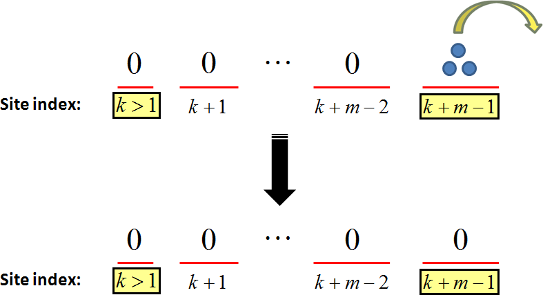
Figure 1: (color online). The non-empty interval $\{k,\ldots,k+m-1\}$ becomes empty if, and only if, all interval sites other than site $k+m-1$ are empty and the particles that occupy site $k+m-1$ hop to site $k+m$.

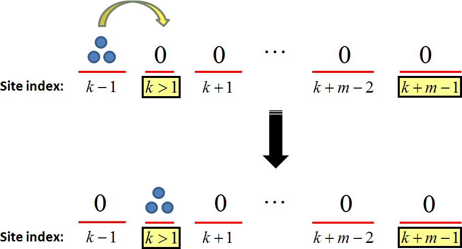
Figure 2: (color online). The empty interval $\{k,\ldots,k+m-1\}$ becomes non-empty if, and only if, site $k-1$ is occupied and the particles that occupy it hop to site $k$.

Eq. (17) remains valid for $m=1$ and $k>1$ provided that we impose the boundary condition

$$P_{0}(t;k,0)\equiv 1\,,$$ (18)

i.e., degenerate intervals (which contain no sites) are by convention always empty. For $k=1$ and $m\geq 1$ the evolution is given by

$$\frac{\partial}{\partial t}P_{0}(t;1,m)=\left[P_{0}(t;1,m-1)-P_{0}(t;1,m)\right]-\lambda P_{0}(t;1,m)\,.$$ (19)

The term $P_{0}(t;1,m-1)-P_{0}(t;1,m)$ appearing on the right-hand side of Eq. (19) manifests the probability that sites $\{1,2,\cdots,m-1\}$ are empty and site $m$ is occupied, in which case the particle cluster at site $m$ might hop (with rate 1) to site $m+1$ and thus leave the interval $\{1,\cdots,m\}$ empty. Also, $P_{0}(t;1,m)$ is the probability that the interval $\{1,\cdots,m\}$ is empty, in which case a particle might arrive to site $1$ (with rate $\lambda$), thus rendering the interval $\{1,\cdots,m\}$ non-empty.

The empty-interval method can be generalized to capture the evolution of the probability $P_{l}(t;k,m)$ that there are exactly $l$ particles at sites $\{k,k+1,\cdots,k+m-1\}$ at time $t$ Coalescence Process ; Kinetic View :

$$P_{l}(t;k,m)\equiv\text{Pr}\bigl{(}L(t;k,m)=l).$$ (20)

The empty-interval probabilities $P_{0}(t;k,m)$ are hence a special case of $P_{l}(t;k,m)$ with $l=0$. The counterparts of Eqs. (17)–(19) are as follows (see Appendices A and B for the derivations). For $k>1$ and $m>1$ the evolution is given by

$$\begin{array}[]{l}\frac{\partial}{\partial t}P_{l}(t;k,m)=\\ \\ +\Bigl{[}P_{l}(t;k,m-1)-2P_{l}(t;k,m)+P_{l}(t;k,m+1)\Bigr{]}\\ \\ -\Bigl{[}P_{l}(t;k,m+1)-P_{l}(t;k-1,m+1)\Bigr{]}\,.\\ \text{ }\end{array}$$ (21)

Equation (21) remains valid for $m=1$ and $k>1$ provided that we impose the boundary condition

$$P_{l}(t;k,0)=\delta_{l,0}\,.$$ (22)

where $\delta_{l,0}$ is the Kronecker delta symbol. Note that, remarkably, Eqs. (21) for $P_{l}(t;k,m)$ do not couple different values of $l$. A coupling enters only through the boundary condition $P_{l}(t;1,m)$ ($m\geq 1$) whose time evolution is given by

$$\begin{array}[]{l}\frac{\partial}{\partial t}P_{l}(t;1,m)=\\ \\ +\Bigl{[}P_{l}(t;1,m-1)-P_{l}(t;1,m)\Bigr{]}\\ \\ -\lambda\Bigl{[}P_{l}(t;1,m)-P_{l-1}(t;1,m)\Bigr{]}\,.\\ \text{ }\end{array}$$ (23)

Note that setting $l=0$ in Eqs. (21)–(23), while taking into account that the probability to observe a negative number of particles is zero by definition, indeed yields Eqs. (17)–(19).

V Continuum limits of the steady-state equations

The main result of this paper is an exact expression for the steady-state solution of Eqs. (17)–(23). Before presenting and deriving this exact solution (see Sections VII and VIII) we provide in the current section a derivation of the asymptotic scaling forms that this solution attains for large values of $k$, i.e., for lattice intervals located far away downstream. As discussed above, some of the asymptotic results presented in this section have been obtained before in Jain using Laplace transform methods. Here we present an alternative “real-space” derivation, which yields new physical insight into the solutions and highlights their universal nature.

The asymptotic analysis of Eqs. (17)–(23) is based on the following continuum-limit assumption: if the steady state probability $P_{l}(k,m)$ changes slowly as a function of the variables $k$ and $m$, then this discrete function may be approximated by one which is continuous both in $k$ and $m$. Thus, one can expand to leading order all terms in the equation around $P_{l}(k,m)$. In this continuum limit, the discrete Laplacian in the first square brackets of Eq. (21) approximately equals a continuous Laplacian, and similarly the second square brackets is approximately $\frac{\partial}{\partial k}P_{l}(k,m)$. Therefore, in the steady-state, where the left-hand side of Eq. (21) vanishes, one finds that $P_{l}(k,m)$ satisfies a diffusion equation where the site number $k$ plays the role of time:

$$\frac{\partial}{\partial k}P_{l}(k,m)=\frac{\partial^{2}}{\partial m^{2}}P_{l}(k,m)\,.$$ (24)

This continuum approximation will be shown a-posteriori to be valid when $k\gg m$.

Equation (24) should be solved with the appropriate boundary conditions in “space” (i.e., in $m$) and “time” (i.e., in $k$). The spatial ($m=0$) boundary condition of Eq. (24) is given in Eq. (22), $P_{l}(k,0)=\delta_{l,0}$. The temporal ($k=1$) initial condition is the steady state solution of Eq. (23), which was found to be ASIP-1 :

$$P_{l}(1,m)=\binom{l+m-1}{l}\biggl{(}\frac{1}{1+\lambda}\biggr{)}^{m}\biggl{(}\frac{\lambda}{1+\lambda}\biggr{)}^{l}\,.$$ (25)

Before proceeding with the study of Eq. (24), let us discuss its relation with the behavior of an ASIP on a ring. Unlike the open boundary ASIP on which we focus, on a ring the steady-state behavior of the model is trivial: a single occupied site circulates throughout the system uni-directionally. The relaxation to this steady-state, however, has an interesting scaling form which has been studied extensively in the context of coagulation models (4)–(5). In particular, it is known that in a spatially homogeneous ring, the probability to find $l$ particles in an interval of $m$ sites evolves (in a continuum limit) according to the diffusion equation (24) with $k$ replaced by time. In other words, as one progresses from left to right along a stationary open-boundary ASIP, the probability to see empty or occupied intervals changes (in space) just like the temporal evolution of the corresponding probability on a ring. This mapping between the two problems provides an interesting physical picture: it suggests that the open-boundary ASIP can be thought of as a sort of a “conveyor belt”, along which the coagulation reaction proceeds. A single steady-state snapshot of the open-boundary ASIP is, in this sense, similar to the entire temporal evolution of the coagulation model on a ring.

It is well known that the diffusion equation on an infinite line has, at times which are large compared with (the square of) the spatial extent of the initial condition, a scaling form of a spreading Gaussian. Having arrived at the diffusion equation (24), it is not too surprising that a similar scaling solution is found for it at large $k$. This solution, however, is not Gaussian, due to the boundary condition (22) which is either a source at the origin when $l=0$ or a sink when $l\geq 1$. In Subsections V.1 and V.2 below, we separately describe and derive the scaling solutions for these two cases. A third, somewhat more subtle, scaling solution is found when considering the joint limit of $l\sim\sqrt{k}\gg 1$. In this case, $k$ is not large enough in comparison with the spatial extent of the “initial condition” (25) in order for the usual scaling of the diffusion equation to apply. Nonetheless, $P_{l}(k,m)$ is found to have a universal scaling form in the variable $l/\sqrt{k}$. This scaling form is discussed in Subsection V.3. The universality of the obtained scaling forms and the conditions under which the continuum approximation is valid are discussed in Subsection V.4.

V.1 The case of $l=0$

As with the usual (probability conserving) diffusion in its late stages, the large $k$ solution of Eq. (24) is given by a scaling form. This form can be found by substituting the ansatz

$$P_{l}(k,m)=k^{-\beta}f\left(\frac{m}{\sqrt{k}}\right)$$ (26)

in Eq. (24), yielding the ordinary differential equation

$$f^{\prime\prime}(u)+\frac{u}{2}f^{\prime}(u)+\beta f(u)=0$$ (27)

for the scaling function $f(u)$, where $u=m/\sqrt{k}$ is the corresponding scaling variable.

In the case of $l=0$ (i.e., the probability to see empty intervals), the boundary condition $P_{0}(k,0)=1$ implies that $\beta=0$ and $f(0)=1$. The solution of Eq. (27) with this boundary condition is given by $f(u)=1+C\,\textrm{erf}(u/2)$ where $C$ is an integration constant, and $\textrm{erf}(x)\equiv 2/\sqrt{\pi}\int_{0}^{x}\exp(-y^{2})dy$ is the error function. For large $u$ this solution approaches $1+C$. Since $\underset{m\to\infty}{\lim}P_{0}(k,m)\to 0$ (i.e., there is a vanishing probability that all sites from $k$ onwards are empty), the constant $C$ must equal $-1$, yielding the scaling solution $f(u)=\textrm{erfc}(u/2)$, i.e.,

$$P_{0}(k,m)\simeq\textrm{erfc}\Bigl{(}\frac{m}{2\sqrt{k}}\Bigr{)},\qquad(m\ll k)$$ (28)

where erfc is the complementary error function defined as $\textrm{erfc}(x)\equiv 1-\textrm{erf}(x)$. Here and in the next two Subsections we indicate in brackets the limiting regime in which the obtained scaling solutions are valid. These are explained below in Subsection V.4.

V.2 The case of $1\leq l\ll\sqrt{k}$

When $l\geq 1$, Eq. (24) should be solved under the absorbing boundary condition $P_{l}(k,0)=0$, which by use of Eq. (26) implies that $f(0)=0$. The corresponding solution of Eq. (27) is

$$f(u)=C\,u\,_{1}F_{1}(\beta+1/2;3/2;-u^{2}/4),$$ (29)

where $C$ is once again an integration constant and ${}_{1}F_{1}(a;b;z)$ is the Kummer hypergeometric function. The values of $\beta$ and $C$ can be determined by using the fact that the quantity $\Lambda=\int_{0}^{\infty}mP_{l}(k,m)dm$ is conserved by the diffusion equation (24) with an absorbing boundary condition, i.e., it can be shown that $d\Lambda/dk=0$ Barenblatt . The discrete counterpart of this conservation law, which results from Eq. (21), states that

$$\Lambda_{l}\equiv\sum_{m=1}^{\infty}(m-1)P_{l}(k,m)$$ (30)

is independent of $k$ in the steady state. For the scaling solution given by the combination of Eqs. (26) and (29), $\Lambda_{l}\simeq k^{1-\beta}\int uf(u)du=k^{1-\beta}\sqrt{4\pi}C,$ and we therefore find that $\beta=1$, for which $f(u)=Cu\exp(-u^{2}/4)$ Abramowitz , and $C=\Lambda_{l}/\sqrt{4\pi}$, i.e.,

$$P_{l}(k,m)\simeq\frac{\Lambda_{l}m}{\sqrt{4\pi}k^{3/2}}e^{-\frac{m^{2}}{4k}}\quad\;(1\leq l\ll\sqrt{k};\,m\ll k).$$ (31)

The value of $\Lambda_{l}$ is found from the initial condition (25) to be

$$\Lambda_{l}=\sum_{m=1}^{\infty}(m-1)P_{l}(1,m)=(l+1)/\lambda^{2}.$$ (32)

To see this, note that up to a multiplication by $\lambda^{-1}$, Eq. (25) is the probability mass function of a sum of $l+1$ independent geometric random variables with mean $\lambda^{-1}$.

Note that the scaling form (31) is valid only in the asymptotic regime when the diffusive length $\sqrt{k}$ is much larger than the spatial spread of the initial condition, which in our case is of the same order of $\Lambda_{l}$. In other words, for any fixed $l\geq 1$, Eq. (31) is a good approximation at “times” where $\sqrt{k}\gg l$. In the next Subsection we examine what happens at “times” $\sqrt{k}\sim l$ which are not large enough for the initial condition to be washed out by the diffusion.

V.3 The case of $l\sim\sqrt{k}$

When $l\sim\sqrt{k}$ and $k$ is not large enough for the diffusion to reach its asymptotic scaling regime, there seems to be no a-priori reason to expect a scaling solution to Eq. (24). However, a closer inspection of the initial condition (25) reveals that such a scaling solution does exist and, surprisingly, is also universal. We now derive this scaling solution; its universality is discussed in the next Subsection.

The key observation now is that the dependence on the number of particles $l$ enters only through the initial condition of Eq. (25), which in the limit we study, and as a function of $m$, is narrowly centered around $m\simeq l/\lambda$. This once again follows from the fact that the initial condition of Eq. (25) is proportional to the probability mass function of a sum of $l+1$ independent geometric random variables with mean $\lambda^{-1}$. Therefore, according to the central limit theorem, the distribution of this sum can be approximated, when $l\to\infty$, by a Gaussian distribution whose mean is given by $\langle m\rangle=(l+1)/\lambda\simeq l/\lambda$. Recalling that the standard deviation scales as $\sqrt{l}$, and is therefore negligible with respect to the mean, we can further approximate the Gaussian probability density function by a Dirac $\delta$ function, i.e.,

$$P_{l}(1,m)\simeq\lambda^{-1}\,\delta(m-l/\lambda).$$ (33)

The solution of the diffusion equation (24) with an absorbing boundary at the origin and the initial condition (33) is found (e.g., by the method of images Images ) to be

$$\begin{array}[]{l}P_{l}(k,m)\simeq\frac{1}{\sqrt{4\pi\lambda^{2}k}}\Bigl{[}e^{-\frac{(m-l/\lambda)^{2}}{4k}}-e^{-\frac{(m+l/\lambda)^{2}}{4k}}\Bigr{]}\\ \text{ }\end{array}\\ (1\ll l\ll k;\,m\ll k).$$ (34)

Equation (34) is a joint scaling solution in the scaling variables $m/\sqrt{k}$ and $l/\sqrt{k}$. If one is further interested in the limit of $m\ll l$, one may expand and obtain to leading order a “thermal dipole”

$$P_{l}(k,m)\simeq\frac{ml}{\sqrt{4\pi}\lambda^{2}k^{3/2}}e^{-\frac{l^{2}}{4\lambda^{2}k}}\qquad(m\ll l\ll k).$$ (35)

Note that, as explained below, Eqs. (34) and (35) are valid not only at the scale of $l\sim\sqrt{k}$, but in fact for all $1\ll l\ll k$.

V.4 Remarks on the scaling solutions

In this Subsection we remark on the limits of validity of the scaling solutions obtained above, and discuss their universality.

The validity of the scaling solutions obtained in the previous sections relies on the continuum approximation of the exact (discrete) Eq. (21) by the continuous Eq. (24). A straightforward calculation shows that the solutions (28), (31), (34), and (35) satisfy

$$P_{l}(k,m+1)-P_{l}(k-1,m+1)=\frac{\partial}{\partial k}P_{l}(k,m)\biggl{[}1+O\Bigl{(}\frac{m}{k},\frac{l}{k}\Bigr{)}\biggr{]}.$$ (36)

and similarly for the discrete $m$-Laplacian. Therefore, the continuum approximation is valid as long as ${m,l\ll k}$. Note in particular that the continuum limit does not require $m$ to be large, and thus the results are valid even for $m=1$.

An important feature of the scaling solutions (28), (31), (34), and (35) is their universality with respect to the details of the how particles arrive at the first site: while the arrival process dictates the distribution of $L(1,m)$, i.e., the initial condition $P_{l}(1,m)$, the scaling solutions are rather insensitive to it. In other words, one may say that the arrival process which feeds particles into the ASIP “conveyor belt” does not affect the load statistics far away downstream. As discussed shortly, universality breaks down for some exotic initial conditions with fat tails, but is otherwise expected to hold for a rather large class of arrival processes.

For the scaling solutions (28) and (31), the origin of universality is easily understood from the diffusion picture of Eq. (24): it is well known that solutions of the diffusion equation converge at late times to scaling functions that are independent of the initial condition (as long as the tail of the initial condition decay rapidly enough) Barenblatt . We now note that $P_{0}(1,m)\leq P_{0}(2,m-1)\leq 1/2^{m-1}$ for any arrival process, as can be clearly seen by considering a limiting scenario in which the arrival process is such that the first site is always occupied. Hence, the initial condition $P_{0}(1,m)$ decays (at least) exponentially fast in $m$ and the pathological case of heavy tails is excluded. As a result, Eq. (28) is not only independent of $\lambda$ in the case of Poissonian arrivals but also completely insensitive to nature of the arrival process altogether.

Equation (31) is also universal, except for the prefactor $\Lambda_{l}$ given by Eq. (32). This prefactor (and only it) depends on the details of the arrival process, and is thus non universal. However, when $l\gg 1$ and for initial conditions which can be approximated by Eq. (33) (see discussion shortly), the prefactor attains the universal form $\Lambda_{l}\simeq l/\lambda^{2}$. This form still “remembers” the mean arrival rate $\lambda$, but is otherwise independent of the arrival process. Its dependence on $\lambda$ is both mathematically unavoidable, due to the conservation of $\Lambda_{l}$, and physically reasonable, as the mean number of particles per site in Eq. (9) depends on $\lambda$. The universality of Eq. (31) breaks down for fat-tailed $P_{l}(1,m)$ for which $\Lambda_{l}$ diverges.

The universality of Eqs. (34) and (35) has a somewhat more subtle origin. As explained above, these scaling forms are valid even though $k$ is not large enough to “wash out” the initial condition $P_{l}(1,m)$. Rather, they emerge exactly when the diffusive length $\sqrt{k}$ is of the order of the initial length scale $\sum_{m}mP_{l}(1,m)\sim l$. The validity of these scaling functions rests on the approximation in Eq. (33), which itself is a result of the central limit theorem. Therefore, the scaling forms (34) and (35) hold whenever the arrival process is such that $L(1,m)$ lends itself to one of the many extensions and generalizations of the central limit theorem. This universality is demonstrated by a specific exactly-solvable example in Appendix C.

The scaling forms (34) and (35) will hold even when the central limit theorem breaks down, and as long as the standard deviation in $L(1,m)$ is negligible with respect to its mean in the limit of $m\rightarrow\infty$. When this is the case, the distribution of $L(1,m)$ is sharply peaked around its mean thus asserting the existence of an approximation of the type appearing in Eq. (33). The basin of attraction for this type of behavior is very large. Indeed, for a general arrival process, Little’s law Wolff asserts that $\left\langle L(1,m)\right\rangle=\bar{\lambda}m$, where $\bar{\lambda}$ is the effective arrival rate (long term average of the number of particles arriving per unit time) and $m$ is the average time a particle spends in the system. On the other hand, fluctuations in $L(1,m)$ are only caused by arrivals to the first site and departures from the last site. And so, given the universality of Eq. (28), if the typical fluctuation due to an arrival event is finite and when $m$ is large, fluctuations in $L(1,m)$ will be dominated by departure events. Hence, the standard deviation in $L(1,m)$ will be of order $\sqrt{m}$ and, most importantly, negligible with respect to the mean.

VI Implications of the inter-particle distribution function

In this section we use the results of Section V to derive the scaling properties of the ASIP which were presented in Section III.

Occupation probabilities. We begin by examining the probability that a site is occupied. Substituting $m=1$ in Eq. (28) and expanding to first order in $k$, we recover Eq. (6). The occupation-number distribution of a single site, $P_{l}(k,1)$, is found by substituting $m=1$ in Eq. (35). Recalling that we have rescaled time such the $\mu=1$, we recover the scaling form reported in Eqs. (7) and (8). In fact, combining (31) with (35) we may write a uniform approximation which is asymptotically exact for all $l\geq 1$ in the limit of $k\gg 1$:

$$P_{l}(k,1)\simeq\frac{\Lambda_{l}}{\sqrt{4\pi}k^{3/2}}e^{-\frac{l^{2}}{4\lambda^{2}k}},$$ (37)

where $\Lambda_{l}$ is given in (32). An interesting picture emerges from the above-mentioned results. Downstream sites with $k\gg 1$ are mostly empty. However, conditioned on being occupied, their occupation is typically of the order of $\sqrt{k}$ [see Eq. (10)], and in fact its distribution has the scaling form of Eq. (37). Below, in Section VIII, we derive an exact expression for this occupation probability which is correct even for small $k$.

Inter-particle distance probability. Another quantity of interest is the inter-particle distance probability $Q(k,m)$, which is defined as the conditional probability that the next occupied site after site $k$ is site $k+m$ given that site $k$ itself is occupied. The scaling solutions found in Section V allow us to calculate $Q(k,m)$. To do so, we first examine the unconditional probability $\left(1-P_{0}(k,1)\right)Q(k,m)$ that sites $k$ and $k+m$ are both occupied and the $m-1$ sites in between the two are empty. This probability is given by

$$\begin{array}[]{l}\left(1-P_{0}(k,1)\right)Q(k,m)=P_{0}(k+1,m-1)\\ \\ -\left[P_{0}(k+1,m)-P_{0}(k,m+1)\right]\\ \\ -\left[P_{0}(k,m)-P_{0}(k,m+1)\right]-P_{0}(k,m+1).\\ \text{ }\end{array}$$ (38)

The first term in Eq. (38) is the probability that sites $\{k+1,\cdots,k+m-1\}$ are empty. From this probability one must subtract: (i) the probability that these sites are empty, site $k$ is occupied and site $k+m$ is empty (the second term, in square brackets); (ii) the probability that these sites are empty, site $k$ is empty and site $k+m$ is occupied (the third term, in square brackets); (iii) the probability that all $m+1$ sites from $k$ to $k+m$ are empty (the last term). Rearranging and passing, as before, to a continuum limit yields

$$\begin{array}[]{l}\left(1-P_{0}(k,1)\right)Q(k,m)=\\ \\ +\left[P_{0}(k,m+1)-2P_{0}(k,m)+P_{0}(k,m-1)\right]\\ \\ -\left[P_{0}(k+1,m)-P_{0}(k,m)-P_{0}(k+1,m-1)+P_{0}(k,m-1)\right]\\ \\ \simeq\left(\frac{\partial^{2}}{\partial m^{2}}-\frac{\partial}{\partial m\partial k}\right)P_{0}(k,m)|_{k,m}\,.\\ \text{ }\end{array}$$ (39)

Substituting Eq. (28) we see that the $\partial^{2}/\partial m^{2}$ term dominates in the large $k$ limit, and we obtain

$$Q(k,m)\simeq\frac{f^{\prime\prime}(u)}{k\left(1-P_{0}(k,1)\right)}=\frac{ue^{-u^{2}/4}}{2\sqrt{k}},$$ (40)

where once again $f(u)=\textrm{erfc}(u/2)$ and $u=m/\sqrt{k}$.

Inter-exit times. For an ASIP in steady state let the random variable $T_{k}$ denote the time elapsing between two consecutive time epochs at which particles exit site $k$. Equation (40) allows us to evaluate the typical order of magnitude of $T_{k}$ in the limit of $k\gg 1$. Indeed, given that site $k$ is occupied, it will take (on average) a single time unit for particles to hop out of it — resulting in a first exit event. On the other hand, we know that $Q(k-m,m)$ is the probability that $k-m$ is the nearest occupied site in the upstream direction. The average distance to the nearest occupied site is hence

$$\begin{array}[]{l}\sum_{m=1}^{k-1}mQ(k-m,m)\simeq\\ \\ \sqrt{k}\overset{\sqrt{k}}{\underset{0}{\int}}\frac{u^{2}e^{-u^{2}/4\left(1-u/\sqrt{k}\right)}}{2\sqrt{1-u/\sqrt{k}}}du\simeq\sqrt{\pi k}\,.\\ \text{ }\end{array}$$ (41)

Thus, $1+\sqrt{\pi k}$ sites on average are to be traversed at an average ‘speed’ of one site per unit time for the second exit event to occur. When $k$ is large, $T_{k}$ is clearly dominated by this traversal time. The error incurred by neglecting the time awaited till the occurrence of the first exit event is negligible and we may safely conclude that $\left\langle T_{k}\right\rangle/\sqrt{\pi k}\simeq 1$.

We can further go on and compute the asymptotic distribution of the inter-exit time. To see how, note that in the limit of $k\gg 1$, the reasoning given above asserts that the probability density of the random variable $T_{k}$ may be approximated by

$$P{}_{T_{k}}(t)\simeq\sum_{m=1}^{k-1}\frac{t^{m}e^{-t}}{m!}Q(k-m,m)$$ (42)

where $t^{m}e^{-t}/m!$ is the probability density for the traversal time of $m+1$ sites. In Appendix D we show that the sum in (42) can be evaluated using a saddle point approximation to yield Eq. (12).

VII Incremental Load Analysis

The analysis conducted so far was based on a continuum limit approximation of Eq. (21) at steady state. Using this approach we were able to analyze homogenous ASIPs and obtain an asymptotic solution for the probabilities $P_{l}(k,m)$ in the limit $k\gg m,l$. We now set forth to obtain an exact solution for this problem. In order to demonstrate the general applicability of the approach described hereinafter we develop it in the context of general ASIPs (not necessarily homogeneous). Setting off from the stochastic law of motion of the incremental load, we go on to derive the boundary value problem which governs its steady state distribution. An algorithm for the solution of this problem is presented along with iterative schemes for the computation of occupation probabilities and factorial moments. In the next section we return to the case of homogeneous ASIPs.

VII.1 The Incremental Load

In this section we revisit the notion of incremental load, which generalizes the notion of overall load. In what follows we consider an infinite lattice with countably many sites, and analyze the ASIP’s incremental load in detail. We consider the lattice interval starting at site $k$ and consisting of $m$ sites — $\{k,k+1,\cdots,k+m-1\}$ ($k,m=1,2,3,\cdots$) — and remind the reader that the ASIP’s incremental loads $L\left(k,m\right)$ and $L\left(t;k,m\right)$ are given by Eqs. (13) and (15), respectively.

Throughout this section we shall employ the natural boundary conditions $L\left(t;k,0\right)=0$ and $L\left(k,0\right)=0$. The Probability Generating Functions (PGFs) of the incremental loads $L\left(k,m\right)$ and $L\left(t;k,m\right)$ are given, respectively, by

$$G\left(z;k,m\right)=\left\langle z^{L\left(k,m\right)}\right\rangle\,,$$ (43)

and

$$G\left(t,z;k,m\right)=\left\langle z^{L\left(t;k,m\right)}\right\rangle\,,$$ (44)

($\left|z\right|\leq 1$). Note that the boundary conditions $L\left(t;k,0\right)=0$ and $L\left(k,0\right)=0$ imply, respectively, the following PGF boundary conditions:

$$G\left(z;k,0\right)=1\text{ \ and \ }G\left(t,z;k,0\right)=1.$$ (45)

VII.2 The Case of $k=1$

In this Subsection we analyze the special case of lattice intervals initiating at the first lattice site $k=1$. This special case yields the overall load which was analyzed in ASIP-1 via the ASIP’s multidimensional PGF. Here we analyze this special case via the method of incremental loads. This serves to illustrate the method which will later be used to derive new results for $k>1$.

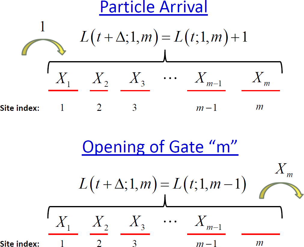
Figure 3: (color online). During the time interval $\left(t,t+\triangle\right)$, the incremental load $L\left(t;1,m\right)$ can change either due to the arrival of a particle to the first site, or due to the opening of gate $m$.

Consider the lattice interval starting at site $1$ and consisting of $m$ sites, and observe its incremental load at times $t$ and $t^{\prime}=t+\Delta$ (where $\Delta\rightarrow 0$). During the time interval $\left(t,t^{\prime}\right)$ exactly two events, illustrated in Figure 3, can change the incremental load. One event is the arrival of a particle to the lattice — in which case the arriving particle enters the first site and hence $L\left(t^{\prime};1,m\right)=L\left(t;1,m\right)+1$; this event occurs with probability $\lambda\Delta+o(\Delta)$. The other event is the opening of gate $m$ — in which case all particles present in site $m$ transit to site $m+1$ and hence $L\left(t^{\prime};1,m\right)=L\left(t;1,m-1\right)$; this event occurs with probability $\mu_{m}\Delta+o(\Delta)$. Note that the boundary condition $L\left(t;1,0\right)=0$ indeed fits in naturally. If neither of these two events take place — a scenario occurring with probability $1-\left(\lambda+\mu_{m}\right)\Delta+o(\Delta)$ — then the incremental load is left unchanged: $L\left(t^{\prime};1,m\right)=L\left(t;1,m\right)$. Thus, the stochastic connection between the incremental loads $L\left(t;1,m\right)$ and $L\left(t^{\prime};1,m\right)$ is given by

$$\begin{array}[]{l}L\left(t^{\prime};1,m\right)=\\ \text{ }\\ \left\{\begin{array}[]{lll}L\left(t;1,m\right)+1&&\text{w.p. \ }\lambda\Delta+o(\Delta)\text{ ,}\\ &\text{ \ }\\ L\left(t;1,m-1\right)&&\text{w.p. \ }\mu_{m}\Delta+o(\Delta)\text{ ,}\\ &\text{ \ }\\ L\left(t;1,m\right)&&\text{w.p. \ }1-\left(\lambda+\mu_{m}\right)\Delta+o(\Delta)\text{ , }\end{array}\right.\end{array}$$ (46)

and we note that “w.p.” is used here as a short hand for the term “with probability”.

Shifting from the incremental loads $L\left(t;1,m\right)$ and $L\left(t^{\prime};1,m\right)$ to their respective PGFs, Eq. (46) yields the following PGF dynamics

$$\begin{array}[]{l}\frac{\partial}{\partial t}G\left(t,z;1,m\right)=\\ \text{ }\\ \left[\lambda\left(z-1\right)-\mu_{m}\right]G\left(t,z;1,m\right)+\mu_{m}G\left(t,z;1,m-1\right)\text{ .}\end{array}$$ (47)

The derivation of Eq. (47) is given in Appendix E. At steady state the time-dependence vanishes, and the differential equation (47) reduces to the steady-state equation

$$G\left(z;1,m\right)=\frac{\mu_{m}}{\mu_{m}+\lambda\left(1-z\right)}G\left(z;1,m-1\right)\text{ .}$$ (48)

A straightforward iterative solution of Eq. (48), using the PGF boundary condition $G\left(z;1,0\right)=1$, yields the following explicit form for the PGF of the incremental load at steady state

$$G\left(z;1,m\right)=\prod_{i=1}^{m}\frac{1}{1+\frac{\lambda}{\mu_{i}}\left(1-z\right)}\,.\text{ }$$ (49)

Note that the terms $\lambda/\mu_{i}$ appearing in Eq. (49) are the ratios of the particles’ inflow rate to the gates’ opening rates, as well as the mean occupancies at steady state ($\lambda/\mu_{i}=\left\langle X_{i}\right\rangle$) ASIP-1 .

Eq. (49) has several important implications. Firstly, Eq. (49) implies that at steady state the overall load $L\left(1,1\right)$ of a single-site ASIP ($n=1$) follows a geometric distribution. Indeed, setting $m=1$ in Eq. (49) yields the PGF of the following geometric probability distribution: $\Pr\left(L\left(1,1\right)=l\right)=(1-p_{1})^{l}p_{1}$ ($l=0,1,2\cdots$), where $p_{1}=\mu_{1}/\left(\mu_{1}+\lambda\right)$. Secondly, the product-form structure of Eq. (49) implies that at steady state the overall load $L\left(1,m\right)$ admits the stochastic representation

$$L(1,m)=\sum_{i=1}^{m}G_{i}\text{ ,}$$ (50)

where $\left\{G_{1},\cdots,G_{m}\right\}$ is a sequence of independent geometrically-distributed random variables: $\Pr\left(G_{i}=l\right)=(1-p_{i})^{l}p_{i}$ ($l=0,1,2,\cdots$), with $p_{i}=\mu_{i}/\left(\mu_{i}+\lambda\right)$ ($i=1,\cdots,m$). The overall load $L\left(1,m\right)$ is hence equal, in law, to the sum of the overall loads of $m$ independent single-site ASIPs with respective parameters $\left(\lambda,\mu_{1}\right),\cdots,\left(\lambda,\mu_{m}\right)$. Thus, the distribution of the overall load $L\left(1,m\right)$ is given by

$$\begin{array}[]{l}P_{l}(1,m)=\Pr\left(L\left(1,m\right)=l\right)=\\ \text{ }\\ \underset{l_{1},\cdots,l_{m}}{\sum}\left(\overset{m}{\underset{i=1}{\prod}}p_{i}(1-p_{i})^{l_{i}}\right)\delta\left(l-\sum_{i}l_{i}\right)\,,\end{array}$$ (51)

where the Dirac $\delta$ function guarantees that $\sum_{i}l_{i}=l$. Thirdly, setting $z=0$ in Eq. (49) (or $l=0$ in Eq. (51)) yields the probability that the lattice interval $\left\{1,\cdots,m\right\}$ is empty

$$P_{0}(1,m)=\Pr\left(L\left(1,m\right)=0\right)=\prod_{i=1}^{m}\frac{\mu_{i}}{\mu_{i}+\lambda}\text{ .}$$ (52)

VII.3 The Case $k>1$

In this Subsection we analyze the general case of lattice intervals initiating at an arbitrary lattice site $k>1$. While the special case $k=1$ could be analyzed via the ASIP’s joint PGF, an analogous analysis of the general case $k>1$ via this method is prohibitively hard. However, as we shall now demonstrate, the analysis of the general case $k>1$ is well attainable following an approach parallel to the one applied in the previous Subsection.

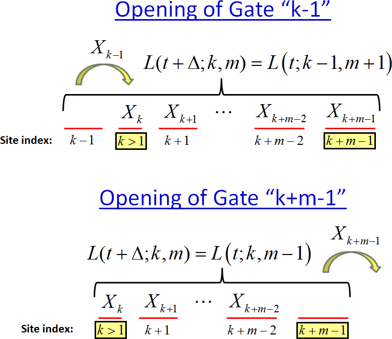
Figure 4: (color online). During the time interval $\left(t,t+\triangle\right)$, the incremental load $L\left(t;k,m\right)$ can change either due to the opening of gate $k-1$ or due to the opening of gate $k+m-1$.

Consider the lattice interval starting at site $k$ ($k>1$) and consisting of $m$ sites, and observe its incremental load at times $t$ and $t^{\prime}=t+\Delta$ (where $\Delta\rightarrow 0$). During the time interval $\left(t,t^{\prime}\right)$ exactly two events, illustrated in Figure 4, can change the incremental load. One event is the opening of gate $k-1$ — in which case all particles present in site $k-1$ transit to site $k$ and hence $L\left(t^{\prime};k,m\right)=L\left(t;k-1,m+1\right)$; this event occurs with probability $\mu_{k-1}\Delta+o(\Delta)$. The other event is the opening of gate $k+m-1$ — in which case all particles present in site $k+m-1$ transit to site $k+m$ and hence $L\left(t^{\prime};k,m\right)=L\left(t;k,m-1\right)$; this event occurs with probability $\mu_{k+m-1}\Delta+o(\Delta)$. As noted in Subsection VII.2, the boundary condition $L\left(t;k,0\right)=0$ fits in naturally. If neither of these two events take place — a scenario occurring with probability $1-\left(\mu_{k-1}+\mu_{k+m-1}\right)\Delta+o(\Delta)$ — then the incremental load is left unchanged: $L\left(t^{\prime};k,m\right)=L\left(t;k,m\right)$. Thus, the stochastic connection between the incremental loads $L\left(t;k,m\right)$ and $L\left(t^{\prime};k,m\right)$ is given by

$$\begin{array}[]{l}L\left(t^{\prime};k,m\right)=\\ \text{ }\\ \left\{\begin{array}[]{ll}L\left(t;k-1,m+1\right)&\text{w.p. \ }\mu_{k-1}\Delta\text{ ,}\\ \\ L\left(t;k,m-1\right)&\text{w.p. \ }\mu_{k+m-1}\Delta\text{ ,}\\ \\ L\left(t;k,m\right)&\text{w.p. \ }1-\left(\mu_{k-1}+\mu_{k+m-1}\right)\Delta\text{ .}\end{array}\right.\end{array}$$ (53)

Shifting from the incremental loads $L\left(t;k,m\right)$ and $L\left(t^{\prime};k,m\right)$ to their respective PGFs, Eq. (53) yields the following PGF dynamics

$$\begin{array}[]{l}\frac{\partial}{\partial t}G\left(t,z;k,m\right)=-\left(\mu_{k-1}+\mu_{k+m-1}\right)G\left(t,z;k,m\right)\\ \\ \text{ }\\ +\mu_{k-1}G\left(t,z;k-1,m+1\right)+\mu_{k+m-1}G\left(t,z;k,m-1\right)\,\,.\end{array}$$ (54)

The derivation of Eq. (54) is given in Appendix F. At steady state the time-dependence vanishes, and the differential equation (54) reduces to the steady-state equation

$$\begin{array}[]{l}G\left(z;k,m\right)=\frac{\mu_{k+m-1}}{\mu_{k-1}+\mu_{k+m-1}}G\left(z;k,m-1\right)\\ \text{ }\\ +\frac{\mu_{k-1}}{\mu_{k-1}+\mu_{k+m-1}}G\left(z;k-1,m+1\right)\text{ .}\end{array}$$ (55)

For any fixed $z$, Eq. (55) defines a two-dimensional boundary value problem for $G\left(z;k,m\right)$. The problem and an algorithm for its solution are illustrated in Figure 5.

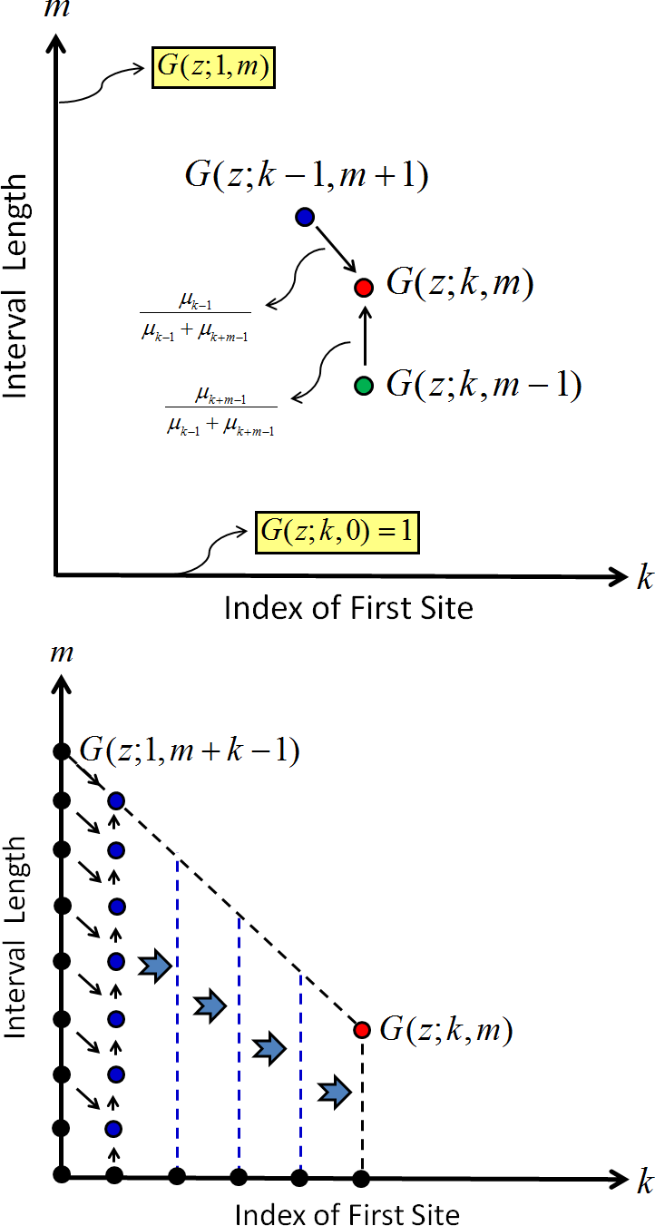
Figure 5: (color online). Top Panel: Equation (55) defines a boundary value problem for $G\left(z;k,m\right)$. The PGF $G\left(z;k,m\right)$ is determined by a weighted average of its southern and northwestern neighbors in the positive quadrant of the $(k,m)$ plane. The boundary PGFs $G\left(z;k,0\right)$ and $G\left(z;1,m\right)$ are given by Eqs. (45) and (49) respectively. Bottom Panel: A three step algorithm can be used in order to solve the boundary value problem for the PGF $G\left(z;k,m\right)$: (i) start at the left boundary and solve for the column that stands to its right; (ii) treat the newly solved column as the new left boundary and iterate; (iii) stop at the $k^{th}$ column and obtain the desired solution.

Equation (55) can also be used to establish an explicit iterative scheme for the computation of the PGF $G\left(z;k,m\right)$ in terms of the PGFs $\left\{G\left(z,k-1,i\right)\right\}_{i=2,...,m+1}$. Specifically:

$$\begin{array}[]{l}G\left(z;k,m\right)=\Pi\left(k,m\right)\\ \text{ }\\ +\Pi\left(k,m\right)\sum_{i=1}^{m}\frac{\mu_{k-1}}{\mu_{k-1}+\mu_{k+i-1}}\frac{G\left(z;k-1,i+1\right)}{\Pi\left(k,i\right)}\text{ ,}\end{array}$$ (56)

where

$$\Pi\left(k,m\right)=\prod_{j=1}^{m}\frac{\mu_{k+j-1}}{\mu_{k-1}+\mu_{k+j-1}}\text{ ,}$$ (57)

and where the boundary condition $G\left(z;1,m\right)$ is given by Eq. (49). The derivation of Eq. (56) is given in Appendix G.

VII.4 Occupation Probabilities and Factorial Moments

Based on the incremental-load results established hitherto, in this Subsection we derive recursive equations for the occupation probabilities and the factorial moments of the incremental loads. We begin with the occupation probabilities, and then turn to the factorial moments.

In terms of the PGF $G\left(z;k,m\right)$ the steady state probability of finding exactly $l$ particles ($l=0,1,2,\cdots)$ in the interval $\left\{k,k+1,\cdots,k+m-1\right\}$ is given by

$$P_{l}\left(k,m\right)=\frac{1}{l!}\left.\frac{d^{l}}{dz^{l}}G\left(z;k,m\right)\right|_{z=0}\,,$$ (58)

with $P_{0}\left(k,m\right)=G\left(0;k,m\right)$. Taking the $l^{th}$ derivative of Eq. (56) with respect to the variable $z$, setting $z=0$ and dividing by $l!$, Eq. (58) yields the following recursion for the occupation probabilities

$$\begin{array}[]{l}\mathrm{P_{\mathit{l}}(\mathit{k,m})}=\Pi\left(k,m\right)\delta_{l,0}\\ \\ \text{ }\\ +\Pi\left(k,m\right)\sum_{i=1}^{m}\frac{\mu_{k-1}}{\mu_{k-1}+\mu_{k+i-1}}\frac{\mathrm{P_{\mathit{l}}(\mathit{k-1,i+1})}}{\Pi\left(k,i\right)}\text{\thinspace.}\end{array}$$ (59)

Equation (59), together with the boundary condition in Eq. (51), establishes an explicit iterative scheme for the computation of the occupation probabilities $\mathrm{P_{\mathit{l}}(\mathit{k,m})}$ in terms of the occupation probabilities $\left\{\mathrm{P_{\mathit{l}}(\mathit{k-\mathrm{1},\mathrm{i}})}\right\}_{i=2,\cdots,m+1}$.

Analogously, one can further derive recursive equations for the factorial moments of the incremental load $L\left(k,m\right)$. In terms of the PGF $G\left(z;k,m\right)$, the factorial moments $M_{l}\left(k,m\right)$ $(l=1,2,3,\cdots)$ are given by

$$M_{l}\left(k,m\right)\equiv\left\langle\overset{l-1}{\underset{i=0}{\prod}}\left(L\left(k,m\right)-i\right)\right\rangle=\left.\frac{d^{l}}{dz^{l}}G\left(z;k,m\right)\right|_{z=1}\,.$$ (60)

Hence, taking the $l^{th}$ derivative of Eq. (56) with respect to the variable $z$ and setting $z=1$, Eq. (60) yields the following recursive equation for the factorial moments

$$\begin{array}[]{l}M_{l}\left(k,m\right)=\\ \text{ }\\ \Pi\left(k,m\right)\sum_{i=1}^{m}\frac{\mu_{k-1}}{\mu_{k-1}+\mu_{k+i-1}}\frac{M_{l}\left(k-1,i+1\right)}{\Pi\left(k,i\right)}\text{ .}\end{array}$$ (61)

Equation (61), together with the boundary condition

$$M_{l}\left(1,m\right)=\left.\frac{d^{l}}{dz^{l}}\prod_{i=1}^{m}\frac{1}{1+\frac{\lambda}{\mu_{i}}\left(1-z\right)}\right|_{z=1}\text{ }$$ (62)

establishes an explicit iterative scheme for the computation of the factorial moments $M_{l}\left(k,m\right)$ in terms of the factorial moments $\left\{M_{l}\left(k-1,i\right)\right\}_{i=2,\cdots,m+1}$.

VIII Incremental Load: Exact Results

In this section we return to the analysis of homogeneous ASIPs and provide exact results for the occupation probabilities and the factorial moments of the incremental load $L(k,m)$. These results are given in terms of the Catalan trapezoid — a generalization of the well known Catalan numbers which appear in many combinatorial settings Catalan . We start in Subsection VIII.1 with a prelude on the Catalan numbers and their extensions, as these numbers will prove instrumental in our analysis. Then, in Subsection VIII.2 we present exact results for incremental load probabilities and factorial moments. We conclude in Subsection VIII.3 in which we provide a derivation of the results presented in VIII.2 along with exact results for the probability generating function of the incremental load.

VIII.1 The Catalan Numbers

Named after the French-Belgian mathematician Eugène Charles Catalan, these numbers arise in various problems in combinatorics. For concreteness we shall henceforth address the Catalan numbers in the following context. Consider a string of numbers composed out of $n$ $(+1)$’s and $n$ $(-1)$’s, arranged in a row from left to right, such that the sum over every initial substring is non-negative. What is the total number of different such strings? The solution to this combinatorial problem is given by the $n^{th}$ Catalan number Catalan :

$$C(n)=\left(\begin{array}[]{c}2n\\ n\end{array}\right)-\left(\begin{array}[]{c}2n\\ n-1\end{array}\right)$$ (63)

$(n=1,2,3,...)$, with $C(0)=1$ by definition. Specifically, the first Catalan numbers are given by $\{1,1,2,5,14,42,132,429,...\}$.

One can generalize the combinatorial problem mentioned above by considering a string of $n$ $(+1)$’s and $k$ $(-1)$’s. In this case, the number of different strings for which the sum over every initial substring is non-negative is given by

$$C(n,k)=\begin{cases}1&\,\,\,k=0\\ \\ \left(\begin{array}[]{c}n+k\\ k\end{array}\right)-\left(\begin{array}[]{c}n+k\\ k-1\end{array}\right)&\,\,\,1\leq k\leq n\\ \\ 0&\,\,\,k>n\end{cases}$$ (64)

$(n=0,1,2,\cdots;k=0,1,2,\cdots)$.

The numbers $C(n,k)$ are referred to — in combinatorial mathematics — as the entries of Catalan’s triangle Catalan ; Catalan's_triangle1 ; Catalan's_triangle2 ; Catalan's_triangle3 . These numbers facilitate the solution to Bertrand’s ballot problem: “In an election where candidate A receives $n$ votes and candidate $B$ receives $k$ votes, what is the probability that $A$ will not trail behind $B$ throughout the entire count of votes?”. Indeed, the answer to Bertrand’s problem is given by the ratio $C(n,k)/\left(\begin{array}[]{c}n+k\\ k\end{array}\right)$.

Catalan’s triangle, illustrated in Table I, has the following iterative construction. By definition, all entries that are positioned on the left boundary of the triangle $(k=0)$ are given by the boundary condition $C(n,0)=1$; in Table I, these entries are highlighted in bold. Entries positioned to the right of the main diagonal $k=n$ are zero; in Table I, these entries are indicated by empty squares. All the other entries of Catalan’s triangle follow the recursion

$$C(n,k)=C(n-1,k)+C(n,k-1)\,,$$ (65)

i.e., each entry is a sum of the entry above it and the entry to its left; in Table I, a specific example, $20+7=27$, is highlighted in magenta. Entries on the diagonal of Catalan’s triangle $(k=n)$ are the Catalan numbers: $C(n,n)=C(n)$; in Table I these entries are highlighted in blue.

$n/k$	0	1	2	3	4	5	6	7
0	1
1	1	1
2	1	2	2
3	1	3	5	5
4	1	4	9	14	14
5	1	5	14	28	42	42
6	1	6	20	48	90	132	132
7	1	7	27	75	165	297	429	429

Table 1: (color online). Some entries of Catalan’s triangle. Entries on the left boundary are highlighted in bold. Null entries positioned to the right of the diagonal $k=n$ are indicated by empty squares. All other entries follow the recursive rule given in Eq. (65). A specific example, $20+7=27$, is highlighted in magenta. The entries on the diagonal of Catalan’s triangle, highlighted in blue, are the Catalan numbers. The second and third diagonals, highlighted in green and red respectively, coincide with the main diagonals of Catalan’s trapezoids of order $m=2$ and $m=3$.

The combinatorial meaning of Eq. (65) and its validity for $1\leq k\leq n$ become immediately clear after conducting a binary partition of all admissible strings according to their last digit $+1$ or $-1$. Indeed, since $k\leq n$ the sum over a string of $n$ $(+1)$’s and $k$ $(-1)$’s is non-negative. Moreover, if the string ends with $+1$ there are exactly $C(n-1,k)$ ways to choose the order of the first $n-1$ $(+1)$’s and $k$ $(-1)$’s such that the sum over every initial substring is non negative. Similarly, if the string ends with a $-1$ there are exactly $C(n,k-1)$ ways to choose the order of the first $n$ $(+1)$’s and $k-1$ $(-1)$’s such that the sum over every initial substring is non negative. Thus, Eq. (65) readily follows.

Further generalizing the combinatorial problem discussed so far we now consider the number of different strings of $n$ $(+1)$’s and $k$ $(-1)$’s for which the sum over every initial substring is larger than, or equal to, a threshold level $1-m$ $(m=1,2,3,\cdots)$. In Catalan Trapezoid it is shown that this number is given by

$$C_{m}(n,k)=\begin{cases}\left(\begin{array}[]{c}n+k\\ k\end{array}\right)&\,\,\,0\leq k<m\\ \\ \left(\begin{array}[]{c}n+k\\ k\end{array}\right)-\left(\begin{array}[]{c}n+k\\ k-m\end{array}\right)&\,\,\,m\leq k\leq n+m-1\\ \\ 0&\,\,\,k>n+m-1\end{cases}$$ (66)

$(n=0,1,2,\cdots;k=0,1,2,\cdots;m=1,2,3,\cdots)$. Note that $C_{1}(n,k)=C(n,k)$ by definition. Indeed, setting $m=1$ in Eq. (66) yields Eq. (64). More generally it can be said that the numbers appearing in Eq. (66) generalize Catalan’s triangle to form a countable family of trapezoid arrays. Fixing the value of the index $m$, we henceforth refer to $C_{m}(n,k)$ as the entries of the Catalan’s trapezoid of order $m$. Catalan’s trapezoid of order $m=2$ and of order $m=3$ are given in Table II.

The iterative construction Catalan’s trapezoids is similar to that of Catalan’s triangle. All elements on the left boundary $(k=0)$ of the trapezoid are given by the boundary condition $C_{m}(n,0)=1$, all elements on the upper boundary of the trapezoid $(n=0;0\leq k\leq m-1)$ are given by the boundary condition $C_{m}(0,k)=1$ and all elements positioned to the right of the diagonal $k=n+m-1$ are set to be zero. The rest of the elements in the trapezoid follow a recursive rule similar to the one given in Eq. (65), albeit replacing the numbers $C(n,k)$ by the numbers $C_{m}(n,k)$:

$$C_{m}(n,k)=C_{m}(n-1,k)+C_{m}(n,k-1)\,,$$ (67)

i.e., each entry is a sum of the entry above it and the entry to its left. Finally we note an important identity that will come in handy later on:

$$C_{m}(n,n+m-1)=C_{1}(n+m-1,n)\,.$$ (68)

That is, the main diagonal of Catlan’s trapezoid of order $m$ coincides with the $m^{th}$ diagonal of Catlan’s triangle. This identity is easily verified by use of Eqs. (64) and (66).

$n/k$	0	1	2	3	4	5	6	7	8
0	1	1
1	1	2	2
2	1	3	5	5
3	1	4	9	14	14
4	1	5	14	28	42	42
5	1	6	20	48	90	132	132
6	1	7	27	75	165	297	429	429
7	1	8	35	110	275	572	1001	1430	1430

$n/k$	0	1	2	3	4	5	6	7	8	9
0	1	1	1
1	1	2	3	3
2	1	3	6	9	9
3	1	4	10	19	28	28
4	1	5	15	34	62	90	90
5	1	6	21	55	117	207	297	297
6	1	7	28	83	200	407	704	1001	1001
7	1	8	36	119	319	726	1430	2431	3432	3432

Table 2: (color online). Some entries of Catalan’s trapezoid of order $m=2$ (top) and $m=3$ (bottom). Entries on the left and upper boundaries are highlighted in bold. Null entries positioned to the right of the diagonal $k=n+m-1$ are indicated by empty squares. All other entries follow the recursive rule given in Eq. (67). Two specific examples, $429+572=1001$ and $117+83=200$, are highlighted in magenta. The main diagonals of Catalan’s trapezoids of order $m=2$ and $m=3$, highlighted in green and red respectively, coincide with the second and third diagonals of Catlan’s triangle (highlighted, in Table I, in green and red respectively).

VIII.2 Occupation Probabilities and Factorial Moments

We are now in a position to present exact steady-state results for both the occupation probabilities and the factorial moments of the incremental load in the homogenous ASIP. In what follows we return to the convention by which $\mu=1$ and $\lambda$ is measured in units of the gate opening rate. The results presented herein will be expressed in terms of the entries of Catalan’s trapezoids $C_{m}(n,k)$. Detailed proofs are given in the following Subsection.

We start with the incremental load $L\left(1,m\right)$. Substituting $p_{i}\rightarrow 1/(1+\lambda)$ in Eq. (51) we obtain the probabilities $P_{l}(1,m)$ given by Eq. (25). Similarly, substituting $\lambda/\mu_{i}\rightarrow\lambda$ in Eq. (62) we obtain the corresponding factorial moments

$$M_{l}\left(1,m\right)=\frac{(m+l-1)!}{(m-1)!}\lambda^{l}\,.\text{ }$$ (69)

We now turn to the incremental load $L(k,m)$, with $k>1$. In what follows we show that the occupation probabilities $P_{l}\left(k,m\right)$ ($l=0,1,2,\cdots)$ are given by

$$\begin{array}[]{l}\mathrm{P_{\mathit{l}}(\mathit{k,m})}=\delta_{l,0}\overset{k}{\underset{j=2}{\sum}}\frac{C_{1}(k+m-j-1,k-j)}{2^{2k+m-2j}}\\ \\ \text{ }\\ +\sum_{j=2}^{k+m-1}\frac{C_{m}(k-2,m+k-1-j)P_{l}(1,j)}{2^{2k+m-2-j}}\,.\end{array}$$ (70)

and that the factorial moments $M_{l}\left(k,m\right)$ ($l=1,2,\cdots)$ are given by

$$\begin{array}[]{l}M_{l}\left(k,m\right)=\sum_{j=2}^{k+m-1}\frac{C_{m}(k-2,m+k-1-j)M_{l}\left(1,j\right)}{2^{2k+m-2-j}}\,.\\ \text{ }\end{array}$$ (71)

We note that the sums in Eqs. (70–71) contain a finite number of explicitly known summands and can thus be used for exact and efficient calculation of $P_{l}\left(k,m\right)$ and $M_{l}\left(k,m\right)$. Moreover, in the case of single-site lattice intervals ($m=1)$ the sums in Eqs. (70–71) can be computed (given Eqs. (25) and (69), and by use of any standard computer algebra software) to be expressed in terms of standard functions. Specifically, the probability distribution and the factorial moments of the random variable $X_{k}$ are given by

$$\begin{array}[]{l}\mathrm{P_{\mathit{l}}(\mathit{k,\mathrm{1}})}=\delta_{l,0}\left(1-\frac{\Gamma(k-1/2)}{\sqrt{\pi}\Gamma(k)}\right)\\ \\ \text{ }\\ +\frac{(1+l)\Gamma(k-3/2)\lambda^{l}}{2\sqrt{\pi}\Gamma(k)(1+\lambda)^{2+l}}\times{}_{2}F_{1}\left(2-k,2+l,4-2k;\frac{2}{1+\lambda}\right)\,,\end{array}$$ (72)

and

$$\begin{array}[]{l}M_{l}\left(k,1\right)=\frac{2^{l}\lambda^{l}\Gamma(1+l/2)\Gamma(k+l/2-1/2)}{\sqrt{\pi}\Gamma(k)}\,,\\ \text{ }\end{array}$$ (73)

where $\Gamma(x)$ and ${}_{2}F_{1}\left(a,b,c;x\right)$ are the Gamma function and hypergeometric function, respectively. For large $k$, an asymptotic analysis of the exact expressions (70) and (72), yields the asymptotic results of Section V. The details of this asymptotic analysis are sketched in Appendix H.

VIII.3 The probability generating function

In this Subsection we derive an expression for the probability generating function $G\left(z;k,m\right)$ and prove the validity of Eqs. (70) and (71). Substituting $\lambda/\mu_{i}\rightarrow\lambda$ in Eq. (49) we see that the probability generating function of the incremental load $L\left(1,m\right)$ is given by

$$G\left(z;1,m\right)=\left(\frac{1}{1+\lambda\left(1-z\right)}\right)^{m}\,.\text{ }$$ (74)

We now turn to derive an expression for $G\left(z;k,m\right)$ in the case of $k>1$. Our derivation is based on an insightful probabilistic interpenetration of the boundary value problem that appears in Eq. (55). An alternative derivation which is algebraic in nature is given in Appendix I.

The first step in our derivation is to note that Eq. (55) is linear with respect to the PGFs that compose it. It follows that $G\left(z;k,m\right)$ can be expressed as a weighted sum over known boundary PGFs of the type $G\left(z;1,m\right)$ and $G\left(z;k,0\right)$. Iterating Eq. (55) in an attempt to find the contribution of a specific boundary PGF to the unknown PGF $G\left(z;k,m\right)$, we consider a path in the first quadrant of the $(k,m)$ plane that: (i) is composed out of steps in the south ($\downarrow$) and northwest ($\nwarrow$) directions only; (ii) connects the point $(k,m)$ with a specific boundary point $(k^{\prime},m^{\prime})$ whose position is associated with the last two arguments of the boundary PGF whose contribution we are trying to assess; (iii) does not pass through any other boundary point. A path that complies with the above-mentioned conditions will henceforth be named a legitimate path.

The number of northwest steps in a legitimate path is given by $k-k^{\prime}$, the number of south steps is given by $k-k^{\prime}+m-m^{\prime}$ and the total number of steps is given by $2k-2k^{\prime}+m-m^{\prime}$. Since we are dealing with a homogeneous ASIP, Eq. (55) asserts that each step in the path contributes a multiplicative factor of exactly $1/2$. The contribution due to a single legitimate path connecting the points $(k,m)$ and $(k^{\prime},m^{\prime})$ is hence $\left(1/2\right)^{2k-2k^{\prime}+m-m^{\prime}}G\left(z;k^{\prime},m^{\prime}\right)$. Taking into account all possible legitimate paths and summing over all boundary points we have

$$\begin{array}[]{l}G\left(z;k,m\right)=\underset{(k^{\prime},m^{\prime})\in boundary}{\sum}\left[\#(k,m,k^{\prime},m^{\prime})\right.\\ \text{ }\\ \left.\left(1/2\right)^{2k-2k^{\prime}+m-m^{\prime}}G\left(z;k^{\prime},m^{\prime}\right)\right]\,,\end{array}$$ (75)

where $\#(k,m,k^{\prime},m^{\prime})$ is the number of legitimate paths that start at $(k,m)$ and end at $(k^{\prime},m^{\prime})$. The idea behind Eq. (75) is illustrated in Figure 6.

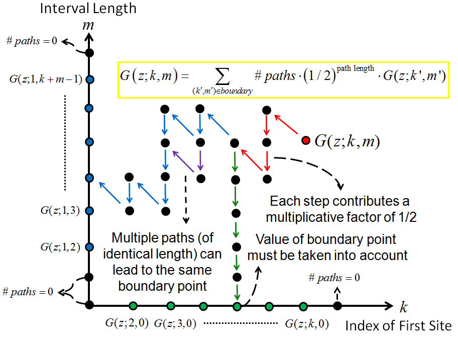
Figure 6: (color online). Expressing $G\left(z;k,m\right)$ as a weighted sum over known boundary functions. All boundary functions must be properly weighted and taken into account. The weight of each boundary function is given by the number of legitimate paths leading to it, multiplied by $1/2$ raised to the power of the path length. Paths are made out of south ($\downarrow$) and northwest ($\nwarrow$) steps only and must not pass through another boundary function except the one lying at the end of the path. Some boundary functions can be reached via several different paths while others cannot be reached at all (the latter are discarded in the computation of the sum).

In order to proceed we consider a random walker that chooses, with equal probability at each step, between a south ($\downarrow$) and northwest step ($\nwarrow$). Assume that the random walker starts its walk at the point $(k,m)$ and let $P_{\text{hit}}^{k,m}(k^{\prime},m^{\prime})$ be the probability that the random walker hits the boundary point $(k^{\prime},m^{\prime})$ before it hits any other boundary point. From this definition it readily follows that

$$P_{\text{hit}}^{k,m}(k^{\prime},m^{\prime})=\#(k,m,k^{\prime},m^{\prime})\cdot\left(1/2\right)^{2k-2k^{\prime}+m-m^{\prime}}\,.$$ (76)

We will now show that

$$P_{\text{hit}}^{k,m}(j,0)=\left(\frac{1}{2}\right)^{2k+m-2j}C_{1}(k+m-j-1,k-j)$$ (77)

($m=1,2,\cdots$;$k=2,3,\cdots$;$j=2,3,\cdots,k$), and that

$$P_{\text{hit}}^{k,m}(1,j)=\left(\frac{1}{2}\right)^{2k+m-2-j}C_{m}(k-2,m+k-1-j)\text{ }$$ (78)

($m=1,2,\cdots$;$k=2,3,\cdots$;$j=2,3,\cdots,k+m-1$).

In every legitimate path connecting the point $(k,m)$ with the point $(j,0)$ ($j=2,3,\cdots,k$) the last step is always directed to the south. The remaining steps — $k-j$ northwest and $k-j+m-1$ south — must be ordered into a path that connects the point $(k,m)$ to the point $(j,1)$ without hitting the south boundary first. Similarly, in every legitimate path connecting the point $(k,m)$ with the point $(1,j)$ ($j=2,3,\cdots,k+m-1$) the last step is always directed to the northwest. The remaining steps — $k-2$ northwest and $k-1+m-j$ south — must be ordered into a path that connects the point $(k,m)$ to the point $(2,j-1)$ without hitting the south boundary first. Recalling the combinatorial interpretation of $C_{m}(n,k)$ one can easily convince himself that $\#(k,m,j,0)=C_{m}(k-j,k-j+m-1)$ and $\#(k,m,1,j)=C_{m}(k-2,k-1+m-j)$. Equation (78) now follows immediately from Eq. (76). Equation (77) follows from Eq. (76) by use of the “diagonal identity” $C_{m}(k-j,k+m-j-1)=C_{1}(k+m-j-1,k-j)$.

The PGF of the incremental load $L(k,m)$ can now be obtained by substituting Eq. (76) into Eq. (75), omitting terms for which $\#(k,m,k^{\prime},m^{\prime})=0$, and utilizing Eqs. (77)-(78) to get

$$\begin{array}[]{l}G\left(z;k,m\right)=\overset{k}{\underset{j=2}{\sum}}G\left(z;j,0\right)\cdot P_{\text{hit}}^{k,m}(j,0)\\ \text{ }\\ +\sum_{j=2}^{k+m-1}G\left(z;1,j\right)\cdot P_{\text{hit}}^{k,m}(1,j)\,.\text{ }\end{array}$$ (79)

Taking the $l^{th}$ derivative of Eq. (79) with respect to the variable $z$ and setting $z=1$, Eq. (71) follows by use of Eq. (60) and the fact that $G\left(z;j,0\right)=P_{0}(j,0)=1$. Substituting Eqs. (77)-(78) into Eq. (79) we conclude that

$$\begin{array}[]{l}G\left(z;k,m\right)=\overset{k}{\underset{j=2}{\sum}}G\left(z;j,0\right)\left(\frac{1}{2}\right)^{2k+m-2j}C_{1}(k+m-j-1,k-j)\\ \\ \text{ }\\ +\sum_{j=2}^{k+m-1}G\left(z;1,j\right)\left(\frac{1}{2}\right)^{2k+m-2-j}C_{m}(k-2,m+k-1-j)\,.\end{array}$$ (80)

The occupation probabilities in Eq. (70) can then be read off from Eq. (80) after substituting $G\left(z;j,0\right)=1$ and $G\left(z;1,j\right)=\overset{\infty}{\underset{l=0}{\sum}}P_{l}(1,j)z^{l}$ .

IX Conclusion

In this paper we studied incremental load probabilities in the ASIP model, analyzed their asymptotic behavior and discussed their implications. Introducing the notion of incremental load, and analyzing it via two complementary approaches — a continuum diffusion-limit approach, and an exact probabilistic-combinatorial approach — we analytically derived expressions for the occupation probabilities of the ASIP’s lattice intervals, their corresponding factorial moments, and for the probability distribution of the ASIP’s inter-exit time. Spanning both exact results and asymptotic behaviors, the analysis presented herein joins the recently published ASIP-3 to provide the most comprehensive description of the ASIP’s steady-state statistics to date.

Our work is yet another step towards a more profound understanding of the ASIP’s complex dynamical behavior, and is part of a long term goal — the elucidation of the ASIP’s steady state distribution in full detail. As an intermediate step, it is natural to turn to the study of correlations between the occupations of several disjoint intervals. The empty interval method was employed in the study of correlations for ASIPs on a ring Coalescence Process , and may thus also prove useful for open boundary ASIPs. This question is especially interesting in light of the picture discussed above of an open ASIP as a ‘conveyor belt’: if a single snapshot of an open boundary ASIP is similar to the temporal evolution of the ASIP on a ring, it would be interesting to examine the relation between two-point correlation functions in the former and two-time correlation functions in the latter.

Other interesting questions remain open, many of which are related to the concept of universality. To this end, it would be very interesting to examine the robustness, and inevitable collapse, of the results presented herein with respect to a large range of perturbations. For example, it would be interesting to further consider the effect of non-homogeneous hopping rates on cluster formation and delineate the conditions under which non-homogeneity is asymptotically averaged out. While some progress in this direction has already been made ASIP-3 , much still remains to be done. Modifying the ASIP a bit, one may ask how does a dependence of the hopping rate on cluster size affect the observed statistics? Another question is what happens when particles arrive to sites other than the first? Finally, the analysis of a generalized ASIP in which hopping times are non-exponential would be both interesting and undoubtedly extremely challenging as it will inevitably require different methods than the ones applied herein.

Appendix A Derivation of Eq. (21)

In this Appendix we present the derivation of Eq. (21). To do so, we define two auxiliary probability functions

$$\begin{array}[]{l}\hat{P}_{l}^{\text{left}}(t;k,m)\equiv\text{Pr}\Bigl{(}L(t;k,m)=l\text{ and $X_{k-1}(t)=0$}\Bigr{)}\\ \\ \hat{P}_{l}^{\text{right}}(t;k,m)\equiv\text{Pr}\Bigl{(}L(t;k,m)=l\text{ and }X_{k+m}(t)=0\Bigr{)}.\\ \text{ }\end{array}$$ (81)

These are the probabilities that sites $\{k,\cdots,k+m-1\}$ are occupied by $l$ particles, and the site immediately to their left/right is empty. Next, note that the probability that sites $\{k-1,\cdots,k+m-1\}$ support $l$ particles and site $k-1$ is not empty is exactly ${P_{l}(t;k-1,m+1)}-\hat{P}_{l}^{\text{left}}(t;k,m)$. Similarly, the probability that sites $\{k,\cdots,k+m-2\}$ support $l$ particles and site $k+m-1$ is not empty is exactly $P_{l}(t;k,m-1)-\hat{P}_{l}^{\text{right}}(t;k,m-1)$. Although the auxiliary probabilities are needed in order to write down the equation of motion for $P_{l}(t;k,m)$,

$$\begin{array}[]{l}\frac{\partial}{\partial t}P_{l}(t;k,m)=\Bigl{(}P_{l}(t;k-1,m+1)-\hat{P}_{l}^{\text{left}}(t;k,m)\Bigr{)}\\ \\ +\Bigl{(}P_{l}(t;k,m-1)-\hat{P}_{l}^{\text{right}}(t;k,m-1)\Bigr{)}\\ \\ -\Bigl{(}P_{l}(t;k,m)-\hat{P}_{l}^{\text{left}}(t;k,m)\Bigr{)}\\ \\ -\Bigl{(}P_{l}(t;k,m)-\hat{P}_{l}^{\text{right}}(t;k,m-1)\Bigr{)}\,,\\ \text{ }\end{array}$$ (82)

they cancel out in Eq. (82) and Eq. (21) readily follows.

Appendix B Derivation of Eq. (23)

The derivation of Eq. (23) is similar to the derivation of Eq. (21) albeit replacing terms corresponding to the entry of particles into the interval from the left (first and third lines of the right hand side of Eq. (82)) with terms corresponding to the arrival of a particle to the first site. The resulting equation is

$$\begin{array}[]{l}\frac{\partial}{\partial t}P_{l}(t;1,m)=\lambda P_{l-1}(t;1,m)-\lambda P_{l}(t;1,m)\\ \\ +\Bigl{(}P_{l}(t;1,m-1)-\hat{P}_{l}^{\text{right}}(t;1,m-1)\Bigr{)}\\ \\ -\Bigl{(}P_{l}(t;1,m)-\hat{P}_{l}^{\text{right}}(t;1,m-1)\Bigr{)}\,.\\ \text{ }\end{array}$$ (83)

Once again, the auxiliary probabilities cancel out, yielding Eq. (23).

Appendix C Universality of Eqs. (34) and (35): an explicit example

In this Appendix we demonstrate how the asymptotic scaling forms (34) and (35) emerge for an explicit example of an ASIP with a generalized arrival process. As explained in Section V.4, the universality is a result of the central limit theorem for the distribution of $L(1,k)$, which leads to Eq. (33). The scaling forms are obtained by showing, for the specific example considered below, that the central limit theorem applies. We also present a formal argument that heuristically explains why the central limit theorem is expected to apply for a much larger class of arrival processes.

Consider an ASIP in which particles may enter the first site not only one by one, but also in batches of $n=2,3,4,\ldots$ particles. The arrival of a batch of $n$ particles is assumed to be a Poisson process with rate $\lambda_{n}$. The occupation of the first site thus increases according to the rule

$$X_{1},X_{2},\cdots\xrightarrow{\lambda_{n}}X_{1}+n,X_{2},\cdots\,$$ (84)

[this is a generalization of Eq. (1)], and otherwise the ASIP dynamics remains unchanged. The goal of the current calculation is to find the initial condition $P_{l}(1,m)$ that is generated by this arrival process, and to analyze the conditions under which the central limit theorem leads to the approximation (33).

The equation equivalent to (23) for this generalized ASIP is

$$\begin{array}[]{l}\frac{\partial}{\partial t}P_{l}(t;1,m)=\Bigl{[}P_{l}(t;1,m-1)-P_{l}(t;1,m)\Bigr{]}\\ \\ -\sum_{n=1}^{\infty}\lambda_{n}\Bigl{[}P_{l}(t;1,m)-P_{l-n}(t;1,m)\Bigr{]}.\\ \text{ }\end{array}$$ (85)

Multiplying by $z^{l}$ and summing over $l$ leads, in the steady state, to

$$\begin{array}[]{l}G(z;1,m-1)-G(z;1,m)=\\ \\ {}[f_{\lambda}(1)-f_{\lambda}(z)]G(z;1,m),\\ \text{ }\end{array}$$ (86)

where $f_{\lambda}(z)$ is the generating function for $\lambda_{n}$:

$$f_{\lambda}(z)\equiv\sum_{n=1}^{\infty}\lambda_{n}z^{n}.$$ (87)

Iterating (86) and using $G(z;1,0)=1$ yields

$$G(z;1,m)=[1+f_{\lambda}(1)-f_{\lambda}(z)]^{-m}.$$ (88)

One observes that the distribution of $L(1,m)$ has a product form and is equal to the distribution of a sum of i.i.d. random variable whose generating function is

$$g(z)\equiv[1+f_{\lambda}(1)-f_{\lambda}(z)]^{-1},$$ (89)

compare with Eq. (74). The central limit theorem for this sum applies when the mean and variance of these i.i.d. variables is finite, i.e., when $g^{\prime}(1),g^{\prime\prime}(1)<\infty$. It is easy to verify that $g^{\prime}(1)=f^{\prime}(1)$ and $g^{\prime\prime}(1)=2f^{\prime\prime}(1)+[f^{\prime}(1)]^{2}$. Thus, as long as $\sum_{n}n^{2}\lambda_{n}<\infty$, one obtains for $m\gg 1$

$$P_{l}(1,m)\sim\delta(l-m\langle\lambda\rangle)=\langle\lambda\rangle^{-1}\delta(m-l/\langle\lambda\rangle),$$ (90)

where we have defined $\langle\lambda\rangle\equiv\sum_{n}n\lambda_{n}$.

Let us now motivate in a heuristic fashion why the central limit theorem is expected to hold for a much larger class of arrival processes. Assume that the arrival process is such that Eq. (86) is replaced by

$$G(z;1,m-1)-G(z;1,m)=\mathcal{A}(z)G(z;1,m),$$ (91)

where $\mathcal{A}(z)$ is a formal notation for the operator associated with the arrival process. The formal solution of this equation is $G(z;1,m)=[1+\mathcal{A}(z)]^{-m}$ [compare with Eq. (88)]. If the operator $[1+\mathcal{A}(z)]^{-1}$ is characterized by a non-vanishing spectral gap, i.e., there is a finite difference between its largest and second-largest eigenvalues, then when $m\to\infty$ one has asymptotically $G(z;1,m)\sim g_{\max}(z)^{m}$, where $g_{\max}(z)$ denotes the largest eigenvalue of $[1+\mathcal{A}(z)]^{-1}$ for some fixed value of $z$. If, in addition, $g_{\max}(z)$ is the PGF of a random variable with finite variance, a central limit theorem holds for $L(1,m)$ and an approximation of the form (33) is valid.

Appendix D Saddle point evaluation of Eq. (42)

In this section we show how Eq. (12) follows by applying a saddle point approximation (also known as Laplace’s method) to the sum in Eq. (42) in the limit $k\to\infty$. The first step is to apply Stirling’s approximation to the probability density of the traversal time

$$\frac{t^{m}e^{-t}}{m!}\simeq\frac{e^{-t+m\log(t/m)+m}}{\sqrt{2\pi m}}\,.$$ (92)

Next, we substitute Eqs. (92) and (40) into Eq. (42) to obtain

$$P{}_{T_{k}}(t)\simeq\sum_{m=1}^{k-1}\frac{e^{-t+m\log(t/m)+m}}{\sqrt{2\pi m}}\frac{me^{-m^{2}/4(k-m)}}{2(k-m)}\,.$$ (93)

Setting $u=m/\sqrt{k}$ we rewrite (93) as

$$P{}_{T_{k}}(t)\simeq\sum_{u}\frac{e^{-t+u\sqrt{k}\log(t/u\sqrt{k})+u\sqrt{k}}}{\sqrt{2\pi u\sqrt{k}}}\frac{ue^{-u^{2}/4\left(1-u/\sqrt{k}\right)}}{2(\sqrt{k}-u)}\,,$$ (94)

where the sum runs over values $u=k^{-1/2},2k^{-1/2},\cdots,k^{1/2}-k^{-1/2}$. We now observe that

$$P_{T_{k}}(\sqrt{k}t)\simeq\sum_{u}\frac{k^{1/4}u^{1/2}}{\sqrt{8\pi}(k-\sqrt{k}u)}e^{\sqrt{k}f(u)}$$ (95)

with

$$f(u)\equiv u\log(t/u)+u-t-u^{2}/(4\sqrt{k}-4u)\,.$$ (96)

For large $k$, the sum in Eq. (95) may be approximated by an integral, which can be evaluated using a saddle point approximation. We thus search for a saddle point $u^{*}$ for which $f^{\prime}(u*)=0$ and find it to be

$$u^{*}=t-t^{2}/2\sqrt{k}+O(k^{-1})\,,$$ (97)

($u^{*}$ is computed to leading in $k$ such that $\underset{k\rightarrow\infty}{\lim}\sqrt{k}f^{\prime}(u^{*})=0$). Evaluating the integral approximation of the sum in Eq. (95) to leading order, we find

$$\begin{array}[]{l}P_{T_{k}}(\sqrt{k}t)\simeq\int_{0}^{\sqrt{k}}\frac{k^{3/4}u^{1/2}}{\sqrt{8\pi}(k-\sqrt{k}u)}e^{\sqrt{k}f(u)}du\\ \\ =\frac{te^{-t^{2}/4}}{2\sqrt{k}}+O(k^{-1})\,.\\ \text{ }\end{array}$$ (98)

We now observe that the probability density function of the normalized inter-exit time $T_{k}/\sqrt{\pi k}$ is related to the probability density function of $T_{k}$ in the following way

$$P_{T_{k}/\sqrt{\pi k}}(t)=\sqrt{\pi k}P_{T_{k}}(\sqrt{\pi k}t)\,.$$ (99)

Equation (12) follows immediately.

Appendix E Derivation of Eq. (47)

Conditioning on the occupancy vector $\mathbf{X}(t)$ and utilizing the Markovian dynamics of Eq. (46) we have

$$\begin{array}[]{l}\left\langle z^{L\left(t^{\prime};1,m\right)}\right\rangle=\left\langle\left\langle z^{L\left(t^{\prime};1,m\right)}|\mathbf{X}(t)\right\rangle\right\rangle\\ \text{ }\\ =\left\{\begin{array}[]{l}(\lambda\Delta)\left\langle z^{L\left(t;1,m\right)+1}\right\rangle\\ +\\ (\mu_{m}\Delta)\left\langle z^{L\left(t;1,m-1\right)}\right\rangle\\ +\\ \left(1-\left(\lambda+\mu_{m}\right)\Delta\right)\left\langle z^{L\left(t;1,m\right)}\right\rangle\\ +\\ o(\Delta)\,\,.\end{array}\right.\end{array}$$ (100)

Equation (47) is obtained after rearranging terms in Eq. (100), dividing by $\Delta$, taking $\Delta\rightarrow 0$ and using the PGF notation of Eq. (43).

Appendix F Derivation of Eq. (54)

Conditioning on the occupancy vector $\mathbf{X}(t)$ and utilizing the Markovian dynamics of Eq. (53) we have

$$\begin{array}[]{l}\left\langle z^{L\left(t^{\prime};k,m\right)}\right\rangle=\left\langle\left\langle z^{L\left(t^{\prime};k,m\right)}|\mathbf{X}(t)\right\rangle\right\rangle\\ \text{ }\\ =\left\{\begin{array}[]{l}(\mu_{k-1}\Delta)\left\langle z^{L\left(t;k-1,m+1\right)}\right\rangle\\ +\\ (\mu_{k+m-1}\Delta)\left\langle z^{L\left(t;k,m-1\right)}\right\rangle\\ +\\ \left(1-(\mu_{k-1}+\mu_{k+m-1})\Delta\right)\left\langle z^{L\left(t;k,l\right)}\right\rangle\\ +\\ o(\Delta)\,\,.\end{array}\right.\end{array}$$ (101)

Equation (54) is obtained after rearranging terms in Eq. (101), dividing by $\Delta$, taking $\Delta\rightarrow 0$ and using the PGF notation of Eq. (43).

Appendix G Derivation of Eq. (56)

We prove Eq. (56) by showing that the probability generating function $G\left(z;k,m\right)$ it defines satisfies Eq. (55). To this end we apply mathematical induction on the index $k$. We start by showing that Eq. (56) holds for $k=2$ and an arbitrary value of $m$. Indeed, for $k=2$ Eq. (56) reads

$$\begin{array}[]{l}G\left(z;2,m\right)=\Pi\left(2,m\right)\\ \\ \text{ }\\ +\Pi\left(2,m\right)\sum_{j=1}^{m}\frac{\mu_{1}}{\mu_{1}+\mu_{1+j}}\frac{G\left(z;1,j+1\right)}{\Pi\left(2,j\right)}\,.\text{ }\end{array}$$ (102)

Substituting Eq. (102) into Eq. (55) and utilizing Eq. (49) we have

$$\begin{array}[]{l}\Pi\left(2,m\right)\left(1+\sum_{j=1}^{m}\frac{\mu_{1}}{\mu_{1}+\mu_{1+j}}\frac{\prod_{i=1}^{j+1}\frac{\mu_{i}}{\mu_{i}+\lambda\left(1-z\right)}}{\Pi\left(2,j\right)}\right)\overset{?}{=}\\ \\ +\frac{\mu_{1+m}}{\mu_{1}+\mu_{1+m}}\Pi\left(2,m-1\right)\left(1+\sum_{j=1}^{m-1}\frac{\mu_{1}}{\mu_{1}+\mu_{1+j}}\frac{\prod_{i=1}^{j+1}\frac{\mu_{i}}{\mu_{i}+\lambda\left(1-z\right)}}{\Pi\left(2,j\right)}\right)\\ \\ \text{ }\\ +\frac{\mu_{1}}{\mu_{1}+\mu_{1+m}}\prod_{j=1}^{m+1}\frac{\mu_{j}}{\mu_{j}+\lambda\left(1-z\right)}\,.\end{array}$$ (103)

Canceling matching terms on both sides of Eq. (103) gives the trivial identity $0=0$ and proves our claim.

We finish the proof by showing that if Eq. (56) holds for $k\geq 2$ it holds for $k+1$ as well. Indeed, replacing $k$ by $k+1$ in Eqs. (55-56) we substitute Eq. (56) into Eq. (55) and obtain

$$\begin{array}[]{l}\Pi\left(k+1,m\right)\left(1+\sum_{j=1}^{m}\frac{\mu_{k}}{\mu_{k}+\mu_{k+j}}\frac{G\left(z;k,j+1\right)}{\Pi\left(k+1,j\right)}\right)\overset{?}{=}\\ \text{ }\\ \\ +\frac{\mu_{k+m}\Pi\left(k+1,m-1\right)}{\mu_{k}+\mu_{k+m}}\left(1+\sum_{j=1}^{m-1}\frac{\mu_{k}}{\mu_{k}+\mu_{k+j}}\frac{G\left(z;k,j+1\right)}{\Pi\left(k+1,j\right)}\right)\\ \\ +\frac{\mu_{k}\Pi\left(k,m+1\right)}{\mu_{k}+\mu_{k+m}}\left(1+\sum_{j=1}^{m+1}\frac{\mu_{k-1}}{\mu_{k-1}+\mu_{k+j-1}}\frac{G\left(z;k-1,j+1\right)}{\Pi\left(k,j\right)}\right)\,.\end{array}$$ (104)

Canceling matching terms on both sides gives

$$\begin{array}[]{l}G\left(z;k,m+1\right)=\\ \text{ }\\ \\ \Pi\left(k,m+1\right)\left(1+\sum_{j=1}^{m+1}\frac{\mu_{k-1}}{\mu_{k-1}+\mu_{k+j-1}}\frac{G\left(z;k-1,j+1\right)}{\Pi\left(k,j\right)}\right)\end{array}$$ (105)

which coincides with Eq. (56) for $G\left(z;k,m+1\right)$ and concludes our proof.

Appendix H Asymptotic analysis of Equation (70)

In this Appendix we sketch the asymptotic analysis of the exact expression for the occupation probabilities (70) and show how the results of Section V, and in particular Eqs. (6), (31)–(32), and (35) can be obtained from it. We concentrate here solely on the case of $m=1$; the calculation for other values of $m$ is similar but somewhat more lengthy.

For the case $m=1,$ the sum in (70) can be rewritten, by substituting the definition (66) and the “initial condition” (25), as

$$P_{0}(k,1)=\sum_{i=0}^{k-2}\binom{2i+1}{i}\frac{1}{2i+1}2^{-(2i+1)}+\\ +\sum_{i=0}^{k-2}\binom{k-1+i}{i}\frac{k-1-i}{k-1+i}2^{-(k-1+i)}(1+\lambda)^{-(k-i)}$$ (106)

for $l=0,$ while for $l\geq 1$ it has the form

$$P_{l}(k,1)=S(2,k),$$ (107)

where we define

$$S(j_{1},j_{2})\equiv \Bigl{(}\frac{\lambda}{1+\lambda}\Bigr{)}^{l}\sum_{j=j_{1}}^{j_{2}}\frac{j-1}{2k-j-1}\binom{2k-j-1}{k-1}\times$$ (108)

$$\times\binom{l+j-1}{l}2^{-(2k-j-1)}(1+\lambda)^{-j}.$$

To obtain these relations we have used the binomial identity $\binom{n-1}{k}-\binom{n}{k}=\frac{n-2k}{n}\binom{n}{k}$.

We first evaluate the sums in Eq. (106) for large $k$. The first sum can be calculated exactly, and equals ${1-\Gamma(k-1/2)/\sqrt{\pi}\Gamma(k)}\simeq 1-1/\sqrt{\pi k}$. The main contribution to the second sum is from values of $i$ which are close to $k$. It can be shown, by expanding the summand for $k\gg k-i$, that the second sum decays to zero as $k^{-3/2}$ and is therefore negligible compared to the first. We thus arrive at Eq. (6).

We now move on to the asymptotic evaluation of (107)–(108) for large $k$. The main contribution to the sum, as shown below, is from values of $j$ which are close to $l.$ Therefore, two cases are treated separately: (i) $l\ll\sqrt{k},$ and (ii) $l=x\sqrt{k}$ with $x=O(1)$.

Case (i), $l\ll\sqrt{k}$. In this case, the sum is evaluated using Stirling’s approximation

$$2^{-(2k-j-1)}\binom{2k-j-1}{k-1}\simeq\sqrt{\frac{2k-j-1}{2\pi(k-j)(k-1)}}e^{-f_{1}(k)},$$ (109)

with

$$f_{1}(k) =(k-1)\log\frac{k-1}{2k-j-1}+(k-j)\log\frac{k-j}{2k-j-1}$$

$$=\frac{j^{2}}{4k}\Bigl{[}1+O\Bigl{(}\frac{j}{k}\Bigr{)}\Bigr{]}.$$ (110)

The term $f_{1}$ in the exponent yields a significant contribution to the summand only for values of $j$ which are comparable with $\sqrt{k}$, while for $j\ll\sqrt{k}$ it is negligible. Accordingly, we split the sum in (107) into two: $P_{l}(k,1)=S(2,N)+S(N+1,k)$, the first running over $j=2,\ldots,N$, and the second over $j=N+1,\ldots k$. Here $N=N(k)$ is chosen in such a way that $l\ll N\ll k$. The first of these sums may be approximated using (109) as

$$S(2,N)\simeq\Bigl{(}\frac{\lambda}{1+\lambda}\Bigr{)}^{l}\sum_{j=2}^{N}\frac{j-1}{\sqrt{4\pi}k^{3/2}}\binom{l+j-1}{l}(1+\lambda)^{-j}.$$

Since $N\gg 1$ and the summand decays exponentially with $j$, replacing the upper boundary in the last sum by $\infty$ results in a negligible error. The sum can now be computed exactly, and yields

$$S(2,N)\simeq\frac{l+1}{\sqrt{4\pi}\lambda^{2}k^{3/2}}.$$

The contribution of the second sum (from $N+1$ to $k$) is negligible as long as $l\ll\sqrt{k}.$ To see this, approximate $\binom{l+j-1}{l}\simeq j^{l+1}/l!$ (which is valid for $j>N\gg l$), and then approximate the sum as an integral:

$$S(N+1,k)\simeq\\ \simeq\Bigl{(}\frac{\lambda}{1+\lambda}\Bigr{)}^{l}\frac{k^{(l-1)/2}}{\sqrt{4\pi}l!}\int_{\frac{N}{\sqrt{k}}}^{\sqrt{k}}y^{l+2}e^{-y^{2}/4-y\sqrt{k}\log(1+\lambda)}dy,$$

where a change of integration variable $y=j/\sqrt{k}$ was made. Once again, we incur a negligible error by approximating the lower and upper integration boundaries as $N/\sqrt{k}\simeq 0$ and $\sqrt{k}\simeq\infty$. By evaluating the integral, it can be shown that $S(N+1,k)\ll S(2,N)$, leading to (31)–(32) (remember that here $m=1$).

Case (ii), $l=x\sqrt{k}$. In this case, since $l\gg 1$, one may employ Stirling’s approximation also for the second binomial coefficient in (108). Replacing as before the sum by an integral with an integration variable $y=j/\sqrt{k}$ leads to

$$P_{l}(k,1)\simeq\int_{0}^{\infty}\Bigl{(}\frac{\lambda}{1+\lambda}\Bigr{)}^{l}\frac{y^{3/2}}{4\pi k^{3/4}\sqrt{x(x+y)}}e^{-\frac{y^{2}}{4}-\sqrt{k}f_{2}(y)}$$

with

$$f_{2}(y)\equiv x\log\frac{x}{x+y}+y\log\frac{y}{x+y}+y\log(1+\lambda).$$

For $\sqrt{k}\gg 1$, the integral can be evaluated using a saddle point approximation: $f_{2}$ has a minimum at $y^{*}=x/\lambda$, where its value is $f_{2}(y^{*})=x\log\lambda/(1+\lambda)$. We therefore obtain the scaling form

$$P_{l}(k,1)\simeq\frac{x}{\sqrt{4\pi}\lambda^{2}k}e^{-x^{2}/4\lambda^{2}}$$

[compare with (35)]. Note that this saddle point calculation carries through to any $1\ll l\ll k$. The results are different, however, at the scale of $l=O(k)$, as the main contribution to the sum (the saddle point) comes from values $j=O(k)$, leading to non-negligible corrections to the calculation due to terms neglected above such as the higher order terms in (110).

Appendix I Derivation of Eq. (80)

In this Appendix we provide an alternative derivation of Eq. (80). The derivation of this Appendix is algebraic in nature and serves to show that the desired result may also be obtained without reference to the probabilistic argumentation presented in the main text. The proof is divided into three parts. In Part I we show that for $k>1$, $G\left(z;k,m\right)$ can be written as

$$\begin{array}[]{l}G\left(z;k,m\right)=\overset{k}{\underset{j=2}{\sum}}\left(\frac{1}{2}\right)^{2k+m-2j}C_{1}(k+m-j-1,k-j)\\ \text{ }\\ +\left(\frac{1}{2}\right)^{2k+m-2}\overset{\infty}{\underset{l=0}{\sum}}A(k,m,l)z^{l}\text{ }\end{array}$$ (111)

where

$$\begin{array}[]{l}A(k,m,l)=\left(\frac{\lambda}{1+\lambda}\right)^{l}\sum_{j_{1}=1}^{m}\sum_{j_{2}=1}^{j_{1}+1}\sum_{j_{3}=1}^{j_{2}+1}\cdot\cdot\cdot\\ \text{ }\\ \cdot\cdot\cdot\sum_{j_{k-2}=1}^{j_{k-3}+1}\sum_{j_{k-1}=1}^{j_{k-2}+1}\binom{j_{k-1}+l}{j_{k-1}}\left(\frac{2}{1+\lambda}\right)^{j_{k-1}+1}\text{ .}\end{array}$$ (112)

In Part two we show that

$$\begin{array}[]{l}A(k,m,l)=\\ \\ \text{ }\\ \sum_{j=1}^{m+k-2}2^{j+1}C_{m}(k-2,m+k-2-j)P_{l}(1,j+1)\,.\end{array}$$ (113)

In Part three we combine Eqs. (111) and (113) to conclude the proof.

I.0.1 Part I

We prove Eq. (111) by induction on $k$. We start by showing that Eq. (111) holds for $k=2$ and an arbitrary value of $m$. Setting $\mu_{i}=\mu$ ($i=1,2,3,\cdots$) in Eq. (56) we have

$$\begin{array}[]{l}G\left(z;k,m\right)=\left(\frac{1}{2}\right)^{m}\\ \text{ }\\ +\sum_{j=1}^{m}\left(\frac{1}{2}\right)^{m+1-j}G\left(z;k-1,j+1\right)\text{ }\end{array}$$ (114)

($k>1$). Setting $k=2$ in Eq. (114) and utilizing Eq. (74) we have

$$\begin{array}[]{l}G\left(z;2,m\right)=\left(\frac{1}{2}\right)^{m}\\ \text{ }\\ \\ +\sum_{j=1}^{m}\left(\frac{1}{2}\right)^{m+1-j}\left(\frac{1}{1+\lambda\left(1-z\right)}\right)^{j+1}\text{ .}\end{array}$$ (115)

Recalling the Taylor expansion

$$\frac{1}{1-x}=\overset{\infty}{\underset{i=0}{\sum}}x^{i}$$ (116)

$|x|<1$, we expand the parenthesis in the second term of Eq. (115) to obtain

$$\begin{array}[]{l}G\left(z;2,m\right)=\left(\frac{1}{2}\right)^{m}\\ \text{ }\\ \\ +\sum_{j=1}^{m}\left(\frac{1}{2}\right)^{m+1-j}\left(\frac{1}{1+\lambda}\right)^{j+1}\left(\overset{\infty}{\underset{i=0}{\sum}}\left(\frac{\lambda z}{1+\lambda}\right)^{i}\right)^{j+1}\text{ .}\end{array}$$ (117)

Noting that

$$\left(\overset{\infty}{\underset{i=0}{\sum}}\left(\frac{\lambda z}{1+\lambda}\right)^{i}\right)^{j+1}=\overset{\infty}{\underset{l=0}{\sum}}\left(\begin{array}[]{c}j+l\\ j\end{array}\right)\left(\frac{\lambda z}{1+\lambda}\right)^{l}$$ (118)

and

$$A(2,m,l)=\left(\frac{\lambda}{1+\lambda}\right)^{l}\sum_{j=1}^{m}\left(\frac{2}{1+\lambda}\right)^{j+1}\left(\begin{array}[]{c}j+l\\ j\end{array}\right)$$ (119)

we substitute Eq. (118) into Eq. (117) to obtain

$$G\left(z;2,m\right)=\left(\frac{1}{2}\right)^{m}+\left(\frac{1}{2}\right)^{m+2}\overset{\infty}{\underset{l=0}{\sum}}A(2,m,l)z^{l}\text{ .}$$ (120)

Noting that $C_{1}\left(m-1,0\right)=1$ ($m=1,2,3,\cdots)$, we see that Eq. (120) identifies with (111) for $k=2$.

We finish the first part of the proof by showing that if Eq. (111) holds for $k\geq 2$ it holds for $k+1$ as well. Indeed, replacing $k$ by $k+1$ in Eq. (114) we substitute Eq. (111) into Eq. (114) and obtain

$$\begin{array}[]{l}G\left(z;k+1,m\right)=\\ \\ +\left(\frac{1}{2}\right)^{m}\left[1+\overset{m}{\underset{i=1}{\sum}}\overset{k}{\underset{j=2}{\sum}}\left(\frac{1}{2}\right)^{2k+2-2j}C_{1}(k-j+i,k-j)\right]\\ \\ \text{ }\\ +\left(\frac{1}{2}\right)^{m+2k}\overset{m}{\underset{i=1}{\sum}}\overset{\infty}{\underset{l=0}{\sum}}A(k,i+1,l)z^{l}\text{ .}\end{array}$$ (121)

Performing an index shift $j\rightarrow k+1-j$, Eq. (121) can be rewritten as

$$\begin{array}[]{l}G\left(z;k+1,m\right)=\\ \\ +\left(\frac{1}{2}\right)^{m}\left[1+\overset{m}{\underset{i=1}{\sum}}\overset{k-1}{\underset{j=1}{\sum}}\left(\frac{1}{2}\right)^{2j}C_{1}(i+j-1,j-1)\right]\\ \\ \text{ }\\ +\left(\frac{1}{2}\right)^{m+2k}\overset{m}{\underset{i=1}{\sum}}\overset{\infty}{\underset{l=0}{\sum}}A(k,i+1,l)z^{l}\text{ .}\end{array}$$ (122)

We now note that Eqs. (65) and (112) imply respectively that

$$C_{1}(j+m-1,j)=\sum_{i=1}^{m}C_{1}(i+j-1,j-1)$$ (123)

and

$$A(k+1,m,l)=\sum_{i=1}^{m}A(k,i+1,l)\,.$$ (124)

Substituting Eqs. (123) and (124) into Eq. (122) we obtain

$$\begin{array}[]{l}G\left(z;k+1,m\right)=\\ \\ +\left(\frac{1}{2}\right)^{m}\left[1+\overset{k-1}{\underset{j=1}{\sum}}\left(\frac{1}{2}\right)^{2j}C_{1}(j+m-1,j)\right]\\ \\ \text{ }\\ +\left(\frac{1}{2}\right)^{m+2k}\overset{\infty}{\underset{l=0}{\sum}}A(k+1,m,l)z^{l}\text{ .}\end{array}$$ (125)

Applying the index shift $j\rightarrow k-j+1$ and noting again that $C_{1}(m-1,0)=1$ ($m=1,2,3,\cdots)$ we conclude that

$$\begin{array}[]{l}G\left(z;k+1,m\right)=\\ \\ +\overset{k+1}{\underset{j=2}{\sum}}\left(\frac{1}{2}\right)^{2k+m+2-2j}C_{1}(k+m-j,k+1-j)\\ \\ \text{ }\\ +\left(\frac{1}{2}\right)^{m+2k}\overset{\infty}{\underset{l=0}{\sum}}A(k+1,m,l)z^{l}\text{ ,}\end{array}$$ (126)

a form which coincides with Eq. (111) for $G\left(z;k+1,m\right)$.

I.0.2 Part II

We will now prove Eq. (113). Examining Eq. (112) it is easy to see that it can be rewritten in the following form

$$\begin{array}[]{l}A(k,m,l)=\sum_{j=1}^{m+k-2}2^{j+1}\#_{k,j}^{m}P_{l}(1,j+1)\,,\\ \text{ }\end{array}$$ (127)

where we have used Eq. (25) and defined

$$\begin{array}[]{l}\#_{k,j}^{m}=\sum_{j_{1}=1}^{m}\sum_{j_{2}=1}^{j_{1}+1}\sum_{j_{3}=1}^{j_{2}+1}\cdot\cdot\cdot\\ \text{ }\\ \cdot\cdot\cdot\sum_{j_{k-2}=1}^{j_{k-3}+1}\sum_{j_{k-1}=1}^{j_{k-2}+1}\delta(j_{k-1},j)\text{ }\end{array}$$ (128)

to be the exact number of times that the running index $j_{k-1}$ in Eq. (112) is equal to $j$ ($j=1,\cdots,m+k-2$).

What can be said about the numbers $\#_{k,j}^{m}$? First, it is fairly straightforward to see that when $k=2$ we have

$$\begin{array}[]{l}\#_{2,j}^{m}=1\end{array}$$ (129)

($m=1,2,\cdots$;$j=1,\cdots,m$). In addition when $j=m+k-2$ we have

$$\begin{array}[]{l}\#_{k,m+k-2}^{m}=1\end{array}$$ (130)

($m=1,2,\cdots$;$k=2,3,\cdots$). Now, for $k>2$ and $1\leq j<m+k-2$ we note that the following recursion relation holds

$$\begin{array}[]{l}\#_{k,j}^{m}=\#_{k-1,j-1}^{m}+\#_{k,j+1}^{m}\,.\end{array}$$ (131)

Indeed, substituting Eq. (128) into Eq. (131) we have

$$\begin{array}[]{l}\#_{k,j}^{m}\overset{?}{=}\sum_{j_{1}=1}^{m}\sum_{j_{2}=1}^{j_{1}+1}\sum_{j_{3}=1}^{j_{2}+1}\cdot\cdot\cdot\sum_{j_{k-2}=1}^{j_{k-3}+1}\delta(j_{k-2},j-1)\\ \text{ }\\ \text{ }\\ +\sum_{j_{1}=1}^{m}\sum_{j_{2}=1}^{j_{1}+1}\sum_{j_{3}=1}^{j_{2}+1}\cdot\cdot\cdot\sum_{j_{k-2}=1}^{j_{k-3}+1}\sum_{j_{k-1}=1}^{j_{k-2}+1}\delta(j_{k-1},j+1)\end{array}$$ (132)

which immediately gives

$$\begin{array}[]{l}\#_{k,j}^{m}\overset{?}{=}\sum_{j_{1}=1}^{m}\sum_{j_{2}=1}^{j_{1}+1}\sum_{j_{3}=1}^{j_{2}+1}\cdot\cdot\cdot\\ \text{ }\\ \cdot\cdot\cdot\sum_{j_{k-2}=1}^{j_{k-3}+1}\left[\delta(j_{k-2},j-1)+\sum_{j_{k-1}=1}^{j_{k-2}+1}\delta(j_{k-1},j+1)\right]\text{ }\end{array}$$ (133)

However, it easy to check that

$$\sum_{j_{k-1}=1}^{j_{k-2}+1}\delta(j_{k-1},j+1)=\left(\sum_{j_{k-1}=1}^{j_{k-2}+1}\delta(j_{k-1},j)\right)-\delta(j_{k-2},j-1)$$ (134)

substituting Eq. (134) into Eq. (133) we recover Eq. (128) and assert the validity of Eq. (131).

We now note that

$$\#_{k,j}^{m}=C_{m}(k-2,m+k-2-j)\,.$$ (135)

Indeed, for $k=2$

$$\begin{array}[]{l}\#_{2,j}^{m}=C_{m}(0,m-j)=1\end{array}$$ (136)

($m=1,2,\cdots$;$j=1,\cdots,m$). In addition, for $j=m+k-2$ we have

$$\begin{array}[]{l}\#_{k,m+k-2}^{m}=C_{m}(k-2,0)=1\end{array}$$ (137)

($m=1,2,\cdots$;$k=2,3,\cdots$). Finally we note that, for $k>2$ and $1\leq j<m+k-2$, Eqs. (131) and (135) imply that

$$\begin{array}[]{l}C_{m}(k-2,m+k-2-j)=C_{m}(k-3,m+k-2-j)\\ \text{ }\\ +C_{m}(k-2,m+k-3-j)\text{ }\end{array}$$ (138)

which together with the boundary conditions specified in Eqs. (136–137) give back the iterative construction of the Catalan trapezoid of order $m$. Substituting Eq. (135) into Eq. (127) we recover prove Eq. (113) and conclude the second part our proof.

I.0.3 Part III

In this part we complete the derivation of Eq. (80). Substituting Eq. (113) into Eq. (111) we have

$$\begin{array}[]{l}G\left(z;k,m\right)=\overset{k}{\underset{j=2}{\sum}}\left(\frac{1}{2}\right)^{2k+m-2j}C_{1}(k+m-j-1,k-j)\\ \text{ }\\ +\overset{\infty}{\underset{l=0}{\sum}}\left[\overset{m+k-2}{\underset{j=1}{\sum}}P_{l}(1,j+1)\cdot\left(\frac{1}{2}\right)^{2k+m-3-j}C_{m}(k-2,m+k-2-j)\right]z^{l}\text{ }\end{array}$$ (139)

where we have utilized the fact that $P_{0}(j,0)=1$. Shifting the index of summation in the inner sum of the second line of Eq. (139) we obtain (80).

References

- (1) S. Reuveni, I. Eliazar and U. Yechiali, Asymmetric Inclusion Process. Phys. Rev. E. 84, 041101, (2011).
- (2) Note that the name ASIP was also used for a different model: S. Grosskinsky, F. Redig and K. Vafayi, Condensation in the inclusion process and related models. Journal of Statistical Physics, Journal of Statistical Physics, 142, 5, 952-974, (2011).
- (3) B. Derrida, E. Domany, and D. Mukamel. An exact solution of the one dimensional asymmetric exclusion model with open boundaries, Journal of Statistical Physics 69, 667 (1992).
- (4) O. Golinelli and K. Mallick, The asymmetric simple exclusion process: an integrable model for non-equilibrium statistical mechanics, J. Phys. A: Math. Gen. 39, 12679, (2006).
- (5) B. Derrida, Non-equilibrium steady states: fluctuations and large deviations of the density and of the current, J. Stat. Mech. P07023 (2007).
- (6) J. R. Jackson, Operations Research 5, 518, (1957).
- (7) J. R. Jackson, Management Science 10, 131, (1963).
- (8) H. Chen and D. D. Yao, Fundamentals of Queueing Networks, Springer, (2001).
- (9) M. F. Neuts, The Busy Period of a Queue with Batch Service. Operations Research 13 815-819 (1965).
- (10) H. Kaspi, O. Kella and D. Perry, Dam processes with state dependent batch sizes and intermittent production processes with state dependent rates. Queueing Systems: Theory and Applications 24 37- 57 (1997).
- (11) J. van der Wal and U. Yechiali, Dynamic Visit-Order Rules for Batch-Service Polling. Probability in the Engineering and Informational Sciences, 17, No. 3, 351, (2003)
- (12) O. Boxma, J. van der Wal and U. Yechiali, Polling with Gated Batch Service. Proceedings of the Sixth International Conference on "Analysis of Manufacturing Systems", Lunteren, The Netherlands, 155, (2007).
- (13) O. Boxma, J. van der Wal and U. Yechiali, Polling with Batch Service. Stochastic Models, 24, No.4, 604, (2008).
- (14) S. Reuveni, I. Eliazar and U. Yechiali, The Asymmetric Inclusion Process: A Showcase of Complexity. Phys. Rev. Lett. 109, 020603, (2012).
- (15) S. Reuveni, I. Eliazar and U. Yechiali, Limit Laws for the Asymmetric Inclusion Process. Phys. Rev. E. 86, 061133, (2012).
- (16) P. L. Krapivsky, S. Redner, and E. Ben-Naim. A kinetic view of statistical physics. Cambridge University Press, Cambridge, UK, 2010.
- (17) D. Ben-Avraham. The coalescence process, , and the method of interparticle distribution functions. In V. Privman, editor, Nonequilibrium Statistical Mechanics in One Dimension, pages 29–50. Cambridge University Press, Cambridge, UK, 2005.
- (18) S. Reuveni, Catalan’s Trapezoids. Under Review.
- (19) K. Thomas, Catalan Numbers with Applications, Oxford University Press, ISBN 0-19-533454-X (2008).
- (20) H.G. Forder, Some Problems in Combinatorics. Math. Gaz. 45, 199, (1961).
- (21) L. W. Shapiro, A Catalan Triangle. Disc. Math. 14, 83, (1976).
- (22) D. F. Bailey, Counting Arrangements of 1’s and -1’s. Math. Mag. 69, 128, (1996).
- (23) K. Jain and M. Barma, Phases of a conserved model of aggregation with fragmentation at fixed sites. Phys. Rev. E. 64, 016107, (2001).
- (24) M., Smoluchowski, Versuch einer mathematischen Theorie der Koagulationskinetik kolloider Lösungen. Z. phys. Chem. 92, (1917).
- (25) I. M. Sokolov, S. B. Yuste, J. J. Ruiz-Lorenzo, and K. Lindenberg. Mean field model of coagulation and annihilation reactions in a medium of quenched traps: Subdiffusion. Phys. Rev. E 80 , 051114, (2009).
- (26) S. B. Yuste, J. J. Ruiz-Lorenzo, and K. Lindenberg. Coagulation reactions in low dimensions: Revisiting subdiffusive A+A reactions in one dimension. Phys. Rev. E 80 , 051114, (2009).
- (27) B. Derrida, V. Hakim, V. Pasquier, Exact First-Passage Exponents of 1D Domain Growth: Relation to a Reaction-Diffusion Model. Phys. Rev. Lett. 75, 751, (1995).
- (28) R. A. Blythe and M. R., Evans, Nonequilibrium steady states of matrix-product form: a solver’s guide. J. Phys. A: Math. Theor. 40, R333-R441, (2007).
- (29) C. T. MacDonald, J. H. Gibbs and A. C. Pipkin, Kinetics of biopolymerization on nucleic acid templates, Biopolymers 6, 1, (1968).
- (30) F. Spitzer, Interaction of Markov Processes. Advances in Mathematics 5, 246, (1970).
- (31) K. Heckmann, Single file diffusion Passive Permeability of Cell Membranes. Biomembranes 3 127 ed. Kreuzer F. and Slegers J. F. G., New York: Plenum, (1972).
- (32) D. G. Levitt, Dynamics of a single-file pore: Non-Fickian behavior, Phys. Rev. A 8 3050 (1973).
- (33) P. M. Richards, Theory of one-dimensional hopping conductivity and diffusion, Phys. Rev. B 16 1393 (1977).
- (34) B. Widom B, J. L. Viovy and A. D. Defontaines, Repton model of gel electrophoresis and diffusion, J. Physique I 1 1759 (1991).
- (35) M. Schreckenberg and D. E. Wolf (ed) Traffic and Granular Flow ’97 (New York: Springer) (1998).
- (36) L. B. Shaw, R.K. Zia and K.H. Lee, Totally asymmetric exclusion process with extended objects: a model for protein synthesis. Phys Rev E 68 021910 (2003).
- (37) S. Reuveni, I. Meilijson, M. Kupiec, E. Ruppin and T. Tuller, Genome-Scale Analysis of Translation Elongation with a Ribosome Flow Mode. PLoS Computational Biology 7(9), e1002127, (2011).
- (38) T. Halpin-Healy and Y. C. Zhang, Kinetic roughening phenomena, stochastic growth, directed polymers and all that, Phys. Rep. 254 215 (1995).
- (39) J. Krug, Origins of scale invariance in growth processes, Adv. Phys. 46 139 (1997).
- (40) R. Bundschuh, Asymmetric exclusion process and extremal statistics of random sequences, Phys. Rev. E 65 031911 (2002).
- (41) S. Klumpp S and R. Lipowsky, Traffic of molecular motors through tube-like compartments, J. Stat. Phys. 113 233 (2003).
- (42) S. F. Burlatsky, G. S. Oshanin, A. V. Mogutov and M. Moreau, Directed walk in a one-dimensional lattice gas. Physics Letters A 166 230-234 (1992).
- (43) S. F. Burlatsky, G. Oshanin, M. Moreau and W. P. Reinhardt, Motion of a driven tracer particle in a one-dimensional symmetric lattice gas. Phys Rev E 54 3165-3172 (1996).
- (44) O. Bénichou, A. M. Cazabat, J. De Coninck, M. Moreau and G. Oshanin, Stokes Formula and Density Perturbances for Driven Tracer Diffusion in an Adsorbed Monolayer. Phys. Rev. Lett. 84 511-514 (2000).
- (45) C. M. Monasterio and Gleb Oshanin, Bias- and bath-mediated pairing of particles driven through a quiescent medium. Soft Matter 7 993-1000 (2011).
- (46) D. Gross, J. F. Shortle, J.M. Thompson amd C.M. Harris, Fundamentals of Queueing Theory, Wiley-Interscience, (2008).
- (47) J. N. Daigle, Queueing Theory with Applications to Packet Telecommunication, Springer, (2004).
- (48) G. Giambene, Queuing Theory and Telecommunications: Networks and Applications, Springer, (2004).
- (49) A. S. Alfa, Queueing Theory for Telecommunications: Discrete Time Modeling of a Single Node System, Springer, (2010).
- (50) G. Ausgabe, Traffic Theory, Kluwer, (2002).
- (51) G. Bolch, S. Greiner, H. de Meer and K. S. Trivedi, Queueing Networks and Markov Chains: Modeling and Performance Evaluation with Computer Science Applications, Wiley-Interscience, 2nd edition, (2006).
- (52) W. J. Stewart, Probability, Markov Chains, Queues, and Simulation: The Mathematical Basis of Performance Modeling, Princeton University Press, (2009).
- (53) R. Nelson, Probability, Stochastic Processes, and Queueing Theory: The Mathematics of Computer Performance Modeling, Springer, (2010).
- (54) A. L. Barabási, The origin of bursts and heavy tails in human dynamics. Nature, 435, 207, (2005)
- (55) A. Vázquez, Exact results for the Barabási model of human dynamics. Phys. Rev. Lett., 95, 248701, (2005).
- (56) J. Walraevens, T. Demoor, T. Maertens and H. Bruneel, Stochastic queueing-theory approach to human dynamics. Phys. Rev. E, 85, 021139, (2012).
- (57) Vidar Frette and P. C. Hemmer, Time needed to board an airplane: A power law and the structure behind it. Phys. Rev. E, 85, 011130, (2012).
- (58) A. Arazi, E. Ben-Jacob and U. Yechiali, Bridging Genetic Networks and Queueing Theory. Physica A, 332, 585, (2004).
- (59) A. Arazi and U. Yechiali, Modeling Genetic Regulatory Systems via a G-Network. Technical Report (2004).
- (60) V. Elgart, T. Jia and R. V. Kulkarni, Applications of Little’s Law to stochastic models of gene expression. Phys. Rev. E, 82, 021901, (2010).
- (61) T. Jia and R. V. Kulkarni, Intrinsic Noise in Stochastic Models of Gene Expression with Molecular Memory and Bursting. Phys. Rev. Lett., 106, 058102, (2011).
- (62) P. Ashwin, C. Lin and G. Steinberg, Queueing induced by bidirectional motor motion near the end of a microtubule. Phys. Rev. E, 82, 051907, (2010).
- (63) B. Tadić and V. Priezzhev, Scaling of avalanche queues in directed dissipative sandpiles. Phys. Rev. E, 62, 3266, (2000).
- (64) Y. Chernyak, M. Chertkov, D. A. Goldberg and K. Turitsyn, Non-Equilibrium Statistical Physics of Currents in Queuing Networks. J. Stat Phys, 140, 819, (2010).
- (65) V. Y. Chernyak, M. Chertkov and N. A. Sinitsyn, The geometric universality of currents. J. Stat. Mech., P09006, (2011).
- (66) N. Merhav and Y. Kafri, Bose-Einstein condensation in large deviations with applications to information systems. J. Stat. Mech., P02011, (2010).
- (67) C. Arita, Queueing process with excluded-volume effect. Phys. Rev. E, 80, 051119, (2009).
- (68) C. Arita, Dynamical analysis of the exclusive queueing process, Phys. Rev. E, 83, 051128 (2011).
- (69) C. Arita and A. Schadschneider, Exact dynamical state of the exclusive queueing process with deterministic hopping. Phys. Rev. E, 84, 051127, (2011).
- (70) G. I. Barenblatt, Scaling, self-similarity, and intermediate asymptotics, Cambridge, Cambridge University Press, (1996).
- (71) M. Abramowitz, I.A. Stegun, Handbook of Mathematical Functions with Formulas, Graphs, and Mathematical Tables, New York, Dover Publications, (1972).
- (72) S. Redner, A Guide to First-Passage Processes, Cambridge University Press, (2001).
- (73) R. W. Wolff, Stochastic Modeling and the Theory of Queues, Prentice-Hall, (1989).