A new method to measure the mass of galaxy clusters

Abstract

The mass measurement of galaxy clusters is an important tool for the determination of cosmological parameters describing the matter and energy content of the Universe. However, the standard methods rely on various assumptions about the shape or the level of equilibrium of the cluster. We present a novel method of measuring cluster masses. It is complementary to most of the other methods, since it only uses kinematical information from outside the virialized cluster. Our method identifies objects, as galaxy sheets or filaments, in the cluster outer region, and infers the cluster mass by modeling how the massive cluster perturbs the motion of the structures from the Hubble flow. At the same time, this technique allows to constrain the three-dimensional orientation of the detected structures with a good accuracy. We use a cosmological numerical simulation to test the method. We then apply the method to the Coma cluster, where we find two galaxy sheets, and measure the mass of Coma to be $M_{\rm vir}=(9.2\pm\,2.4)\times\,10^{14}\rm M_{\odot}$, in good agreement with previous measurements obtained with the standard methods.

1 Introduction

The picture of the large-scale structures reveals that matter in the Universe forms an intricate and complex system, defined as “cosmic web” (Zeldovich et al., 1982; Shandarin & Zeldovich, 1983; Einasto et al., 1984; Bond et al., 1996; Aragón-Calvo et al., 2010).

First attempts of mapping the three-dimensional spatial distribution of galaxies in the Universe (Gregory et al., 1978; de Lapparent et al., 1986; Geller & Huchra, 1989; Shectman et al., 1996), as well as more recent large galaxy surveys (Colless et al., 2003; Tegmark et al., 2004; Huchra et al., 2005), display a strongly anisotropic morphology. The galactic mass distribution seems to form a rich cosmos containing clumpy structures, as clusters, sheets and filaments, surrounded by large voids (van de Weygaert & Bond, 2008). A similar cosmic network has emerged from cosmological N-body simulations of the Dark Matter distribution (Bond et al., 1996; Aragón-Calvo et al., 2007; Hahn et al., 2007).

The large scale structures are expected to span a range of scales that goes from a few up to hundreds of megaparsec. Despite the many well-established methods to identify clusters and voids, there is not yet a clear characterization of filaments and sheets. Due to their complex shape, there is not a common agreement on the definition and the internal properties of these objects (Bond et al., 2010). Moreover, their detection in observations is extremely difficult due to the projection effects. Nevertheless, several automated algorithms for filament and sheet finding, both in 3D and 2D, have been developed (Novikov et al., 2006; Aragón-Calvo et al., 2007; Sousbie et al., 2008; Bond et al., 2010). Several galaxy filaments have been detected by eye (Colberg et al., 2005; Porter et al., 2008) and Dark Matter filaments have also been detected from their weak gravitational lensing signal (Dietrich et al., 2012). Powerful methods for the cosmic web classification, are based on the study of the Hessian of the gravitational potential and the shear of the velocity field (Hahn et al., 2007; Hoffman et al., 2012).

From the qualitative point of view, several elaborate theories have been proposed. The cosmic web nature is intimately connected with the gravitational formation process. In the standard model of hierarchical structure formation, the cosmic structure has emerged from the growth of small initial density fluctuations in the homogeneous early Universe (Peebles, 1980; Davis et al., 1985; White & Frenk, 1991). The accretion process involves the matter flowing out of the voids, collapsing into sheets and filaments, and merging into massive clusters. Thus, galaxy clusters are located at the intersection of filaments and sheets, which operate as channels for the matter to flow into them (van Haarlem & van de Weygaert, 1993; Colberg et al., 1999). The innermost part of clusters tends to eventually reach the virial equilibrium.

As result of this gravitational collapse, clusters of galaxies are the most recent structures in the Universe. For this reason, they are possibly the most easy large-scale systems to study. Mass measurement of galaxy clusters is of great interest for understanding the large-scale physical processes and the evolution of structures in the Universe (White et al., 2010). Moreover, the abundance of galaxy clusters as function of their mass is crucial for constraining cosmological models: the cluster mass function is an important tool for the determination of the amount of Dark Matter in the Universe and for studying the nature and evolution of Dark Energy (Haiman et al., 2001; Cunha et al., 2009; Allen et al., 2011). The oldest method for the cluster mass determination is based on the application of the virial theorem to positions and velocities of the cluster members (Zwicky, 1933). This method suffers from the main limitation that the estimated mass is significantly biased when the cluster is far from virialization. More recent and sophisticated techniques also rely strongly on the assumption of hydrostatic or dynamical equilibrium. The cluster mass profile can be estimated, for example, from observations of density and temperature of the hot X-ray gas, through the application of the hydrostatic equilibrium equation (Ettori et al., 2002; Borgani et al., 2004; Zappacosta et al., 2006; Schmidt & Allen, 2007; Host & Hansen, 2011). Another approach is based on the dynamical analysis of cluster-member galaxies and involves the application of the Jeans equations for steady-state spherical system. (Girardi et al., 1998; Łokas & Mamon, 2003; Łokas et al., 2006; Mamon & Boué, 2010). Additional cluster mass estimators have been proposed, which are independent of the cluster dynamical state. A measurement of the total cluster mass can be achieved by studying the distortion of background galaxies due to gravitational lensing (Mandelbaum et al., 2010; Lombriser, 2011). The lensing technique is very sensitive to the instrument resolution and the projection effects. The caustic method has been proposed by Diaferio (1999). This method requires very large galaxy surveys, in order to determine the caustic curve accurately. Therefore, the development of new techniques and the combination of different independent methods, is extremely useful for providing a more accurate cluster mass measurement.

The Coma cluster of galaxies (Abell 1656) is one of the most extensively studied system of galaxies (Biviano, 1998), as the most regular, richest and best-observed in our neighborhood. The X-ray observations have provided several mass estimates (Hughes, 1989; Watt et al., 1992), obtained by assuming hydrostatic equilibrium. Dynamical mass measurements with different methods, based on the assumption of dynamical equilibrium, are reported in (The & White, 1986; Łokas & Mamon, 2003). Geller et al. (1999) perform a dynamical measurement of the Coma cluster, using the caustic method, and weak lensing mass estimates of Coma have been carried on by Kubo et al. (2007) and Gavazzi et al. (2009).

In the present paper we propose a new method for estimating the mass of clusters. We intend to infer total cluster mass from the knowledge of the kinematics in the outskirts, where the matter has not yet reached equilibrium. The key of our method is the analysis of filamentary and sheetlike structures flowing outside the cluster. We apply our method for the total virial mass estimate to the Coma cluster, and we compare our result with some of the previous ones in the literature. Our method also provides an estimation of the orientation of the structures we find, in the three dimensional space. This can be useful to identify a major merging plane, if a sufficient number of structures are detected and at least three of them are on the same plane.

The paper is organized as follows. In section 2 we derive the relation between the velocity profile of galaxies in the outer region of clusters and the virial cluster mass. In section 3 we propose a method to detect filaments or sheets by looking at the observed velocity field. In section 4 we test the method to a cosmological simulated cluster-size halo and we present the result on the mass measurement. In section 5 we present the structures we find around the Coma cluster and the Coma virial mass determination.

2 Mass estimate from the radial velocity profile

Galaxy clusters are characterized by a virialized region where the matter is approximately in dynamical equilibrium. The radius that delimitates the equilibrated cluster, i.e. the virial radius $r_{\rm v}$, is defined as the distance from the centre of the cluster within which the mean density is $\Delta$ times the critical density of the Universe $\rho_{c}$. The virial mass is then given by

$$M_{\rm v}=\frac{4}{3}\pi\,r_{\rm v}^{3}\,\Delta\,\rho_{c}\,.$$ (1)

The critical density is given by

$$\rho_{c}=\frac{3\,H^{2}}{8\pi\,G}\,,$$ (2)

where $H$ is the Hubble constant and $G$ the universal gravitational constant.

The circular velocity $V_{\rm v}$ at $r=r_{\rm v}$, i.e. the virial velocity, is defined as

$$V_{\rm v}^{2}=\frac{G\,M_{\rm v}}{r_{\rm v}}.$$ (3)

The immediate environments of galaxy clusters outside the virial radius are characterized by galaxies and groups of galaxies which are falling towards the cluster centre. These galaxies are not part of the virialized cluster, but they are gravitationally bound to it. The region where the infall motion is most pronounced extends up to three or four times the virial radius (Mamon et al., 2004; Wojtak et al., 2005; Rines & Diaferio, 2006; Cuesta et al., 2008; Falco et al., 2013). At larger scales, typically beyond $6-10\,r_{\rm v}$, the radial motion of galaxies with respect to the cluster centre, is essentially dominated by the Hubble flow. In the transition region between the infall regime and the Hubble regime, the galaxies are flowing away from the cluster, but they are still gravitationally affected by the presence of its mass. At this scale, the gravitational effect of the inner cluster mass is to perturb the simple Hubble motion, leading to a deceleration.

The total mean radial velocity of galaxies outside clusters is therefore the combination of two terms:

$$\overline{v}_{\rm r}(r)=H\,r+\overline{v}_{\rm p}(r)\,,$$ (4)

the pure Hubble flow, and a mean negative infall term $\overline{v}_{\rm p}(r)$, that accounts for the departure from the Hubble relation. Section (2.1) is dedicated to the characterization of the function $\overline{v}_{\rm p}(r)$.

The mean infall velocity depends on the halo mass, being more significant for larger mass haloes. Therefore, we can rewrite equation (4) as

$$\overline{v}_{\rm r}(r,M_{\rm v})=H\,r+\overline{v}_{\rm p}(r,M_{\rm v})\,,$$ (5)

where we include the dependence on the virial mass $M_{\rm v}$.

Therefore, once we know the relation between $\overline{v}_{\rm p}$ and $M_{\rm v}$, equation (5) can be used to infer the virial mass of clusters.

In the next section, we will derive the equation that connects the peculiar velocity of galaxies $\overline{v}_{\rm p}$ with the virial mass of the cluster $M_{\rm v}$.

2.1 Radial infall velocity profile

Simulations have shown a quite universal trend for the radial mean velocity profile of cluster-size haloes, when normalized to their virial velocities (Prada et al., 2006; Cuesta et al., 2008). This feature can be seen, for example, in Fig. 1, where the median radial velocity profile for three samples of stacked simulated haloes is displayed. The units in the plot are the virial velocity $V_{\rm v}$ and virial radius $r_{\rm v}$. The virial masses for the samples are: $M_{\rm v}=0.8\times 10^{14}\,M_{\odot}$ (blue, triple-dot dashed line), $M_{\rm v}=1.1\times 10^{14}\,M_{\odot}$ (green dot dashed line), $M_{\rm v}=4.7\times 10^{14}\,M_{\odot}$ (red dashed line). The cosmological N-body simulation we used is described in section 4.

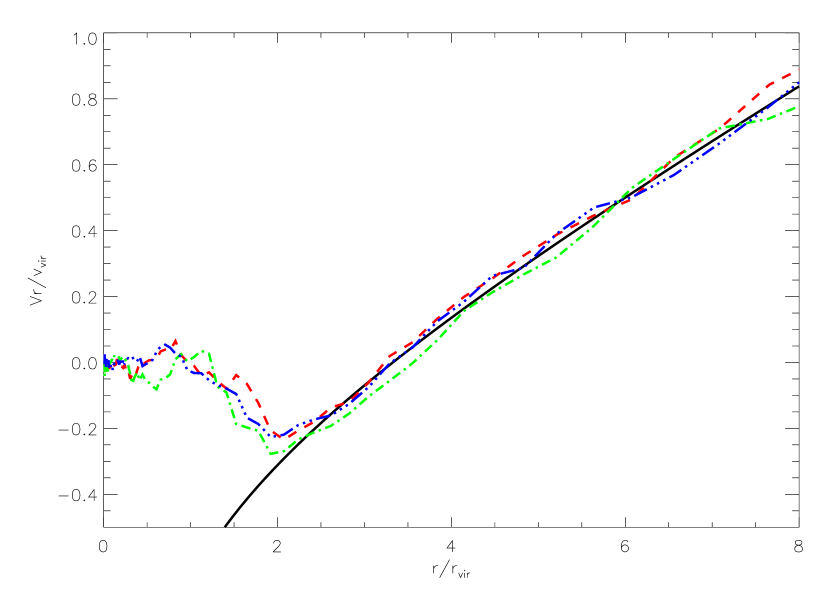
Figure 1: Median radial velocity profile for three samples of stacked simulated halos. The virial masses for the samples are: $M_{\rm v}=0.8\times 10^{14}\,M_{\odot}$ (blue, triple-dot dashed line), $M_{\rm v}=1.1\times 10^{14}\,M_{\odot}$ (green dot dashed line), $M_{\rm v}=4.7\times 10^{14}\,M_{\odot}$ (red dashed line). The black solid line is our simultaneous fit to the three profiles.

In order to derive an approximation for the mean velocity profile, the spherical collapse model has been assumed in several works (Peirani & de Freitas Pacheco, 2006, 2008; Karachentsev & Nasonova (2010), Kashibadze; Nasonova et al., 2011). Here we make a more conservative choice. We parametrize the infall profile using only the information that it must reach zero at large distances from the halo centre, and then we fit the universal shape of the simulated haloes profiles. Therefore, we don’t assume the spherical infall model.

In the region where the Hubble flow starts to dominate and the total mean radial velocity becomes positive, a good approximation for the infall term is

$$\overline{v}_{\rm p}(r)\approx\,-v_{0}\,\left(\frac{r}{r_{\rm v}}\right)^{-b}\,,$$ (6)

with $v_{0}=a\,V_{\rm v}$, where $V_{\rm v}$ is the virial velocity, and $r_{\rm v}$ is the virial radius.

We fit equation (6) to the three profiles in Fig. 1 simultaneously, with $a$ and $b$ as free parameters. The fit is performed in the range $r=3-8\,\rm r_{\rm v}$. The best fit is the black solid line, corresponding to parameters: $a=0.8$ and $b=0.42$.

This allows to fix a universal shape for the mean velocity of the infalling matter, as function of the virial velocity, i.e. the virial mass, in the outer region of clusters.

3 Filaments and sheets around galaxy clusters

The method we propose for measuring the virial cluster mass, consists in using only observed velocities and distances of galaxies, which are outside the virialized part of the cluster, but whose motion is still affected by the mass of the cluster. Given the dependence of the infall velocity on the virial mass, we wish to estimate $M_{\rm v}$ by fitting the measured velocity of galaxies moving around the cluster with equations (5) and (6).

To this end, we need to select galaxies which are sitting, on average, in the transition region of the mean radial velocity profile. For the fit to be accurate, the galaxies should be spread over several megaparsec in radius.

Observations give the two-dimensional map of clusters and their surroundings, namely the projected radius of galaxies on the sky $R$, and the component of the galaxy velocities along the line of sight $v_{\rm los}$. The reconstruction of the radial velocity profile would require the knowledge of the radial position of the galaxies, i.e. the radius $r$. The velocity profile that we infer from observations is also affected by the projection effects. If the galaxies were randomly located around clusters, the projected velocities would be quite uniformly distributed, and we would not see any signature of the radial velocity profile. The problem is overcome because of the strong anisotropy of the matter distribution. At several megaparsec away from the cluster centre, we will select collections of galaxies bound into systems, as filaments or sheets. The presence of such objects can break the spatial degeneracy in the velocity space.

In sections (3.1) and (3.2), we explain in details how such objects can be identified as filamentary structures in the projected velocity space.

3.1 Line of sight velocity profile

In order to apply the universal velocity profile (6) to observations, we need to transform the 3D radial equation (4) in a 2D projected equation. We thus need to compute the line of sight velocity profile $v_{\rm los}$ as function of the projected radius $R$.

Let’s consider a filamentary structure forming an angle $\alpha$ between the 3-dimensional radial position of galaxy members $r$ and the 2-dimensional projected radius $R$. Alternatively, let’s consider a sheet in the 3D space lying on a plan with inclination $\alpha$ with respect to the plan of the sky (see the schematic Fig. 2).

The transformations between quantities in the physical space and in the redshift space are

$$R=\cos\alpha\,r$$ (7)

for the spatial coordinate, and

$$v_{\rm los}(R)=\sin\alpha\,v_{\rm r}(r)$$ (8)

for the velocity.

By inserting equation (5) in equation (8), we obtain the following expression for the line of sight velocity in the general case:

$$v_{\rm los}(R,\alpha,M_{\rm v})=\sin\alpha\,\left[H\,\frac{R}{\cos\alpha}+v_{\rm p}\left(\frac{R}{\cos\alpha},M_{\rm v}\right)\right].$$ (9)

If we use our model for the infall term, given by equation (6), the line of sight velocity profile in equation (9) becomes

$$v_{\rm los}(R,\alpha,M_{\rm v})=\sin\alpha\,\left[H\,\frac{R}{\cos\alpha}-a\,V_{\rm v}\,\left(\frac{R}{\cos\alpha\,r_{\rm v}}\right)^{-b}\right]\,.$$ (10)

By using equation (10), it is, in principle, possible to measure both the virial cluster mass $M_{\rm v}$ and the orientation angle $\alpha$ of the structure. In fact, if we select a sample of galaxies which lie in a sheet or a filament, we can fit their phase-space coordinates ($R,v_{\rm los}$) with equation (10), where only two free parameters ($\alpha,M_{\rm v}$) are involved. The identification of structures and the accuracy on the mass estimate require a quite dense sample of galaxies observed outside the cluster.

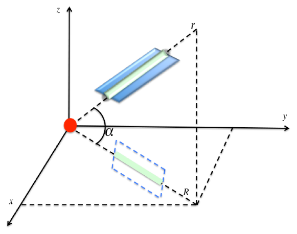
Figure 2: Schematic drawing of a filament or a sheet in 3D with inclination $\alpha$ between the radial distance $r$ and the projected radius $R$. The cluster is represented by the red circle in the centre of the frame. The $z$-axis corresponds to the observer line of sight.

3.2 Linear structures in the velocity field

Our interest here is thus in finding groups of galaxies outside clusters, that form a bound system with a relatively small dispersion in velocity, and that lie on a preferential direction in the 3D space. In particular, we are interested in such objects when they are far enough from the cluster, to follow a nearly linear radial pattern in the velocity space, corresponding to a decelerated Hubble flow.

We expect these objects to form filament-like structures in the projected velocity space. In fact, if we apply the formula in equation (9) to galaxies with the same orientation angle $\alpha$ within a small scatter, the radial velocity shape given by equation (5) is preserved. Thus, these galaxies can be identified as they are collected on a line in the observed velocity space.

Nevertheless, we can look at the structure in the 2D map (the ($x,y$) plane in Fig. 2). If all the selected galaxies lie on a line, within a small scatter, also in the ($x,y$) plane, they can be defined as a filament. If they are confined in a region within a small angular aperture, they might form a sheet (see the Fig. 2). Complementary papers will analyze properties of such sheets (Brinckmann et al., 2013; Sparre, 2013; Wadekar & Hansen, 2013).

We want to point out here that Fig. 2 describes the ideal configuration for filaments and sheets to have a quasi-linear shape in the observed velocity plane. Therefore, not all the filaments and sheets will satisfy this requirement, i. e. not all the structures outside clusters can be detected by looking at the velocity field.

Our method for identifying these objects is optimized towards structures which are narrow in velocity space, while still containing many galaxies, and therefore which are closer to face-on than edge-on. It consists in selecting a region in the sky, and looking for a possible presence of an overdensity in the corresponding velocity space. We will describe the method in details in the next section.

4 Testing the method on Cosmological Simulation

As a first test of our method, we apply it to a cluster-size halo from a cosmological N-body simulation of pure Dark Matter (DM).

The N-body simulation is based on the $WMAP3$ cosmology. The cosmological parameters are $\Omega_{\rm M}=0.24$ and $\Omega_{\Lambda}=0.76$, and the reduced Hubble parameter is $h=0.73$. The particles are confined in a box of size $160\,h^{-1}$ Mpc. The particle mass is $3.5\times\,10^{8}\,\rm M_{\odot}$, thus there are $1024^{3}$ particles in the box. The evolution is followed from the initial redshift $z=30$, using the MPI version of the ART code (Kravtsov et al., 1997; Gottloeber & Klypin, 2008). The algorithm used to identify clusters is the hierarchical friends-of-friends (FOF) with a linking length of 0.17 times the mean interparticle distance. The cluster centres correspond to the positions of the most massive substructures found at the linking length eight times shorter than the mean interparticle distance. We define the virial radius of halos as the radius containing an overdensity of $\Delta=93.8$ relative to the critical density of the Universe. More details on the simulation can be found in (Wojtak et al., 2008).

For our study, we select, at redshift $z=0$, a halo of virial quantities $M_{\rm v}=4.75\times\,10^{14}\,\rm M_{\odot}$, $\rm r_{\rm v}=2.0\,Mpc$ and $V_{\rm v}=1007.3\,\rm km/s$.

We treat the DM particles in the halo as galaxies from observations. The first step is to project the 3D halo as we would see it on the sky. We consider three directions as possible lines of sight. For each projection, we include in our analysis all galaxies in the box $x=[-20,20]\,\rm Mpc$ and $y=[-20,20]\,\rm Mpc$, where $x,y$ are the two directions perpendicular to the line of sight.

The method described in the next section is applied to all the three projections.

4.1 Identification of filaments and sheets from the velocity field

Our goal is to find structures confined in a relatively small area in the $(x,y)$ plane. To this end, we split the spatial distribution into eight two-dimensional wedges (for example in Figure 3 the orange points represent one of the wedges) and we look at each of them in the $(R,v_{\rm los})$-space (for example in Fig. 4 we look at the orange wedge in Fig. 3, in the velocity space), where we aim to look for overdensities.

We confine the velocity field to the box: $v_{\rm los}=[-4000,4000]\,\rm km/s$ and $\rm R=[4,20]\,\rm Mpc$, and we divide the box into $50$ cells, $4\,\rm Mpc$ large and $400\,\rm km/s$ high.

For each of the selected wedges, we want to compare the galaxy number density $n_{i}$ in each cell $i$, with the same quantity calculated for the the rest of the wedges in the same cell. More precisely, in each cell, we calculate the mean of the galaxy number density of all the wedges but the selected one. This quantity acts as background for the selected wedge, and we refer to it as $n^{bg}_{i}$.

In Fig. 3, the wedge under analysis is represented by the orange points, and the background by the green points. We exclude from the background the two wedges adjacent to the selected one (gray points in Fig. 3). We need this step because, if any structure is sitting in the selected wedge, it might stretch to the closest wedges.

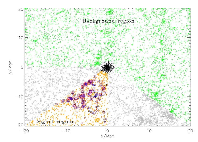
Figure 3: Two-dimensional projection of the simulation box, centered on the selected simulated halo. The black triangles represent the particles inside the virial radius of the halo. The orange points belong to one of the eight wedges we select in the $(x,y)$ plane. The background for the selected wedge is given by the green crosses. The two wedges adjacent to the selected wedge, gray diamonds, are excluded from the analysis. In the selected wedge, we identify a sheet that is represented by the red circles. The blue squares correspond to the total overdensity we find in the wedge, with the method described in the text.

The overdensity in the cell $i$ is evaluated as

$$m_{i}=\frac{n_{i}-n^{bg}_{i}}{n^{bg}_{i}}\,,$$ (11)

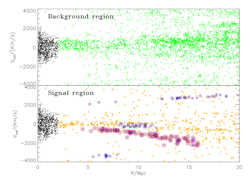
Figure 4: Line of sight velocity $v_{\rm los}$ as function of the projected distance $R$ from the centre of the simulated halo. Upper panel: The background in the analysis is represented by the green crosses. The black triangles are all the particles within the virial radius. Bottom panel: The orange points represent our signal, i.e. the selected wedge. The blue points correspond to the overdensity in the wedge. The only almost straight inclined line is shown in red circles. We identify this filamentary-like structure as a sheet.

and we calculate the probability density $p(m_{i})$ for the given wedge. We take only the cells in the top $1\,\sigma$ region of the probability density distribution, i.e. where the integrated probability is above $(100-16.8)\%$, in order to reduce the background noise. Among the galaxies belonging to the selected cells, we take the ones lying on inclined lines within a small scatter, while we remove the unwanted few groups which appear as blobs or as horizontal strips in the $(R,v_{\rm los})$-space. We apply this selection criterion because we are interested in extended structures which have a coherent flow relative to the cluster.

This method leaves us with only one structure inside the wedge in Fig. 3 (red points). It is a sheet, as it appears as a two-dimensional object on the sky, opposed to a filament which should appear one-dimensional. We see such sheet only in one of the three projections we analyse. The bottom panel of Fig. 4 shows the velocity-distance plot corresponding to all the galaxies belonging to the selected wedge (orange points), while the selected strips of galaxies are shown as blue points. The desired sheet (red points) is an almost straight inclined line crossing zero velocity roughly near 5-10 Mpc and contains 88 particles. The background wedges are displayed in the upper panel of Fig. 4.

4.2 Analysis and result

Having identified one sheet around the simulated halo, we can now extract the halo mass, using the standard Monte Carlo fitting methods. We apply the Monte Carlo Markov chain to the galaxies belonging to the sheet. The model is given by equation (10), where the free parameters are $(\alpha,\rm M_{\rm vir})$. We set $\Delta=93.8$ and $H=73\,\rm km/(s\,Mpc)$, as these are the values set in the cosmological simulation. We run one chain of $5000$ combinations of parameters and then we remove the burn-in points.

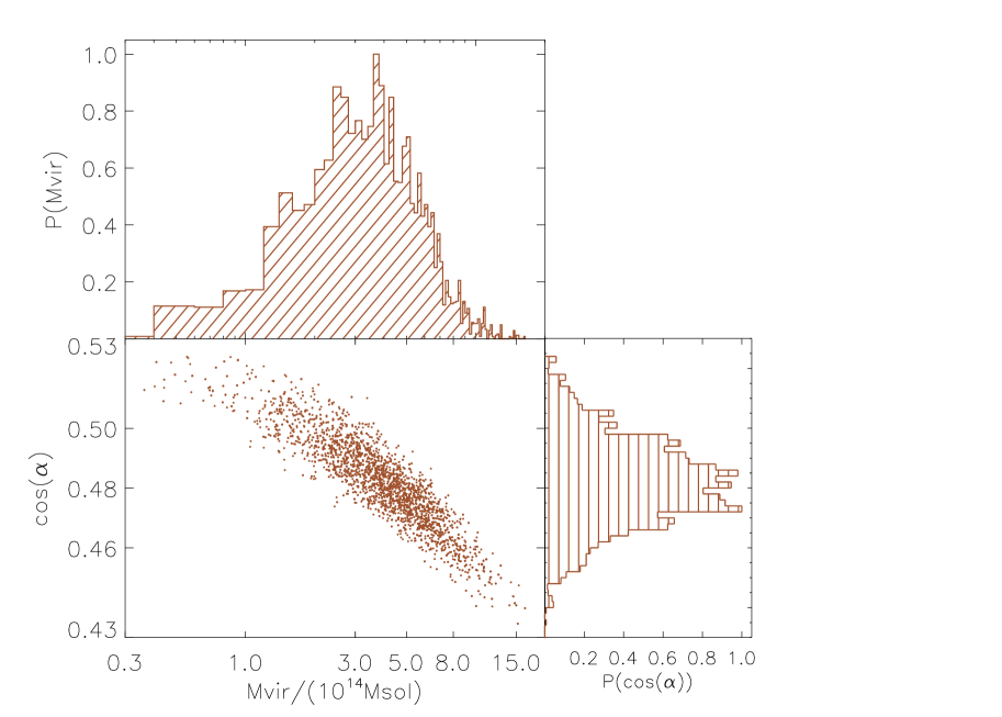
Figure 5: Result of the Monte Carlo Markov chain applied to the sheet found outside the simulated halo. Central panel: Scatter plot of the two free parameters (${\rm cos}(\alpha),M_{\rm vir}$) obtained by the MCMC chain. Upper panel: Probability density function of the virial mass. Left panel: Probability density function of the viewing angle. The initial number of points is 5000 and we remove the points of burn-in. The mean value for the virial mass and the cosine of the angle are $M_{\rm vir}=(4.3\pm\,2.2)\times\,10^{14}\,\rm M_{\odot}$ and ${\rm cos}(\alpha)=0.48\pm\,0.02$, which are comparable to the true halo virial mass $M_{\rm vir}=4.75\times\,10^{14}\,\rm M_{\odot}$ and angle ${\rm cos}(\alpha)=0.5$.

In Fig. 5 we show the scatter plot on the plane of the two parameters, and the one-dimensional probability distribution functions of the virial mass and the orientation angle. The mean value for the virial mass is $M_{\rm vir}=(4.3\pm\,2.2)\times\,10^{14}\,\rm M_{\odot}$, which is comparable to the true halo virial mass $M_{\rm vir}=4.75\times\,10^{14}\,\rm M_{\odot}$. The mean value for the cosine of the angle between $R$ and $r$ is ${\rm cos}(\alpha)=0.48\pm\,0.02$, corresponding to $\alpha=-1.07\pm\,0.02$ rad. In Fig. 6 we show the sheet in the 3D space (blue points). The best fit for the plane where the sheet is laying, is shown as the green plane, and the corresponding angle is $\alpha=-1.05$ rad, giving ${\rm cos}(\alpha)=0.5$. Our estimation is thus consistent, within the statistical error, with the true orientation of the sheet in 3D.

Although our method provides the correct halo mass and orientation angle within the errors, the results slightly underestimate the true values, for both parameters. Systematic errors on the mass and angle estimation might be due to the non ideal shape of the structures. The sheet we find has finite thickness, and it is not perfectly straight in the 3D space. The closer the detected structure is to an ideal infinite thin and perfectly straight object, the smaller the errors would be. Another problem might reside in the assumption of spherical symmetry. The median radial velocity profile of a stack of haloes, might slightly differ from the real velocity profile of each individual halo. Intrinsic scatter of the simulated infall velocity profiles leads to additional systematic errors on the determination of the best fitting parameters. Our estimate of this inaccuracy yields $50\%$ for the virial mass and $2.5\%$ for the angle.

The presence of this systematic is confirmed by Fig. 7. The bottom panel represents our result of the sheet analysis, when using a fit to the real mean radial velocity of the halo, which is shown in the upper panel. The best fit parameters to the radial velocity profile of the halo, with equation (6), are $a=1.5$ and $b=0.89$. In Fig. 7, the black solid line is the fit to the halo velocity profile (red dashed line) and the green dot-dashed line is the universal velocity profile used in the previous analysis. The two profiles overlap in the range $\approx\,3-5\,r_{\rm v}$, but they slightly differ for larger distances, where our sheet is actually sitting. Replacing the universal radial velocity profile with the true one, eliminates the small off set caused by the departure of the two profiles. In the new analysis, the mean value for the virial mass is $M_{\rm vir}=(4.67\pm\,1.9)\times\,10^{14}\,\rm M_{\odot}$, while the mean value for the cosine of the angle between $R$ and $r$ is ${\rm cos}(\alpha)=0.5\pm\,0.01$. They are in very good agreement with the true values of the parameters $M_{\rm vir}=4.7\times\,10^{14}\,\rm M_{\odot}$ and ${\rm cos}(\alpha)=0.5$.

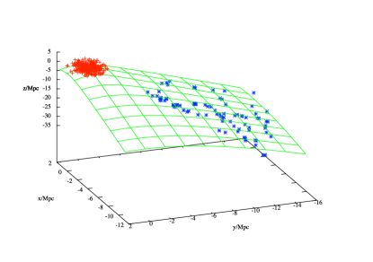
Figure 6: The sheet we found outside the simulated halo in the three-dimensional space. The $z$-axis corresponds to the line of sight direction. The blue points represent the particles belonging to the sheet, and the green plane is the best fit for the sheet’s plane, corresponding to $\alpha=-1.05$ (${\rm cos}(\alpha)=0.5$) rad. The red points represent the particles within the virial radius of the halo.

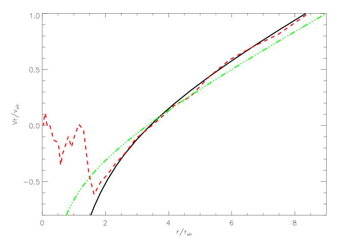
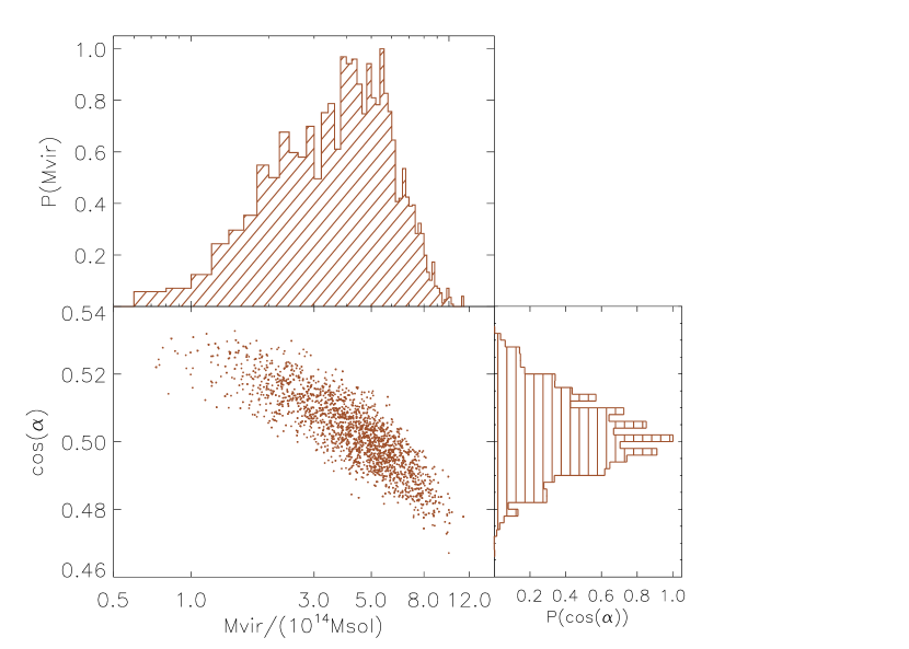
Figure 7: The top figure shows the median radial velocity profile for the simulated halo (red dashed line). The black solid line is our fit to the profile. The green dot-dashed line is the universal radial profile showed in Fig. 1. The bottom figure shows the result of the Monte Carlo Markov chain applied on the sheet found around the simulated halo, using the fit to the mean velocity profile of the halo (top figure). Central panel: Scatter plot of the two free parameters (${\rm cos}(\alpha),M_{\rm vir}$) obtained by the MCMC chain. Upper panel: Probability density function of the virial mass. Left panel: Probability density function of the viewing angle. The initial number of points is 5000 and we remove the points of burn-in. The mean value for the virial mass is $M_{\rm vir}=(4.67\pm\,1.9)\times\,10^{14}\,\rm M_{\odot}$, which is very close to the true halo virial mass $M_{\rm vir}=4.75\times\,10^{14}\,\rm M_{\odot}$. The mean value for the cosine of the angle is ${\rm cos}(\alpha)=0.5\pm\,0.01$, in agreement with the real value ${\rm cos}(\alpha)=0.5$.

5 Result on Coma Cluster

In this section, we will apply our method to real data of the Coma cluster.

We search for data in and around the Coma Cluster in the SDSS database (Abazajian et al., 2009). We take the galaxy NGC 4874 as the centre of the Coma cluster (Kent & Gunn, 1982), which has coordinates: RA=12h59m35.7s, Dec=+27deg57’33”. We select galaxies within 18 degrees from the position of the Coma centre and with velocities between 3000 and 11000 km/s. The sample contains 9000 galaxies.

We apply the method for the identification of structures outside clusters to the Coma data. We detect two galactic sheets in the environment of Coma. We denote our sheets as sheet 1 and sheet 2.

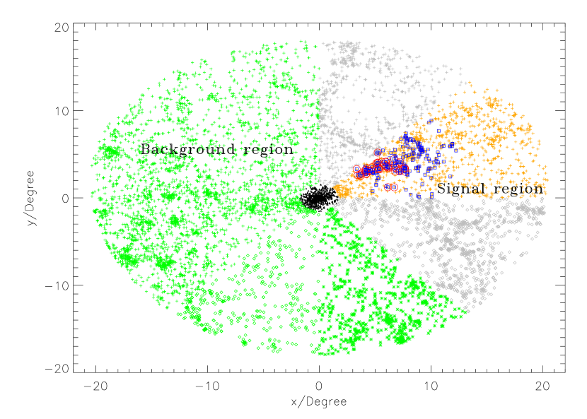
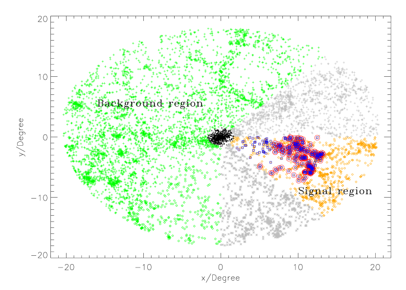
Figure 8: Sky map of the Coma cluster. The top figure shows the sheet 1 and the bottom figure shows the sheet 2. The black triangles represent the particles inside the virial radius of Coma. The orange points belong to one of the eight wedges we select in the $(x,y)$ plane. The background for the selected wedge is given by the green crosses. The two wedges adjacent to the selected wedge, gray diamonds, are excluded from the analysis. In the selected wedge, we identify a sheet that is represented by the red circles. The blue squares correspond to the total overdensity we find in the wedge, with the method described in the text.

Fig. 8 shows the Coma cluster and its environment up to 18 degrees from the cluster centre. The number of galaxies with spectroscopically measured redshifts within $2.5\,$Mpc, which is roughly the virial radius of Coma, is 748. These galaxies are indicated as black triangles. The sheets are the red circles. The upper panel refers to the sheet 1, which contains 51 galaxies. The bottom panel refers to the sheet 2, which is more extended and contains 228 galaxies. In Fig. 9, we show the sheets in the velocity space. They both appear as inclined straight lines. The sheet 1 goes from $\approx\,7\,$Mpc to $\approx\,14\,$Mpc. As the velocities are negative, the sheet is between us and Coma. The sheet 2 goes from $\approx\,11\,$Mpc to $\approx\,22\,$Mpc. As the velocities are positive, the sheet is beyond Coma.

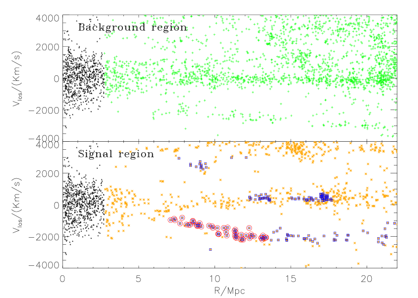
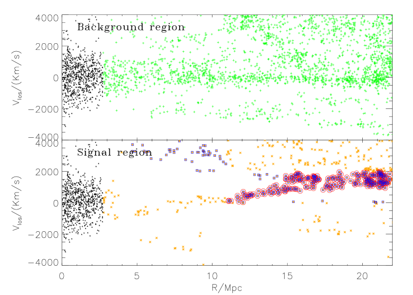
Figure 9: Line of sight velocity $v_{\rm los}$ as function of the projected distance $R$ from the centre of Coma. The velocities are scaled by the velocity of Coma $v_{\rm Coma}=4000$km/s. The top figure shows the sheet 1 and the bottom figure shows the sheet 2. Upper panels: The background in the analysis is represented by the green crosses. The black triangles are all the galaxies within $r=2.5$ Mpc. Bottom panel: The orange points represent the signal, i.e. the selected wedge. The blue points correspond to the overdensity. The almost straight inclined lines are shown in red circles. We identify these filamentary-like structures as sheets.

As we did for the cosmological simulation, we have removed the collections of galaxies which are horizontal groups in ($R,v_{\rm los}$)-space by hand. For example, in the case of the sheet 1 in the upper panel of Fig. 9, we define the sheet only by including the inclined pattern and therefore, by excluding the horizontal part of the strip.

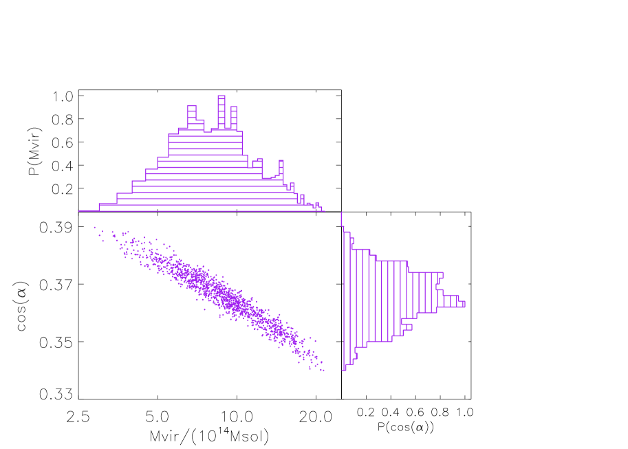
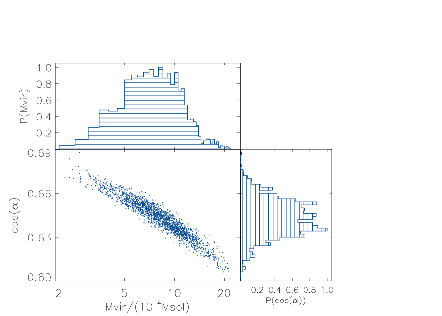
Figure 10: Result of the Monte Carlo Markov chain applied to the two sheets found outside the Coma cluster. The top figure refers to the sheet 1 and the bottom figure refers to the sheet 2. Central panels: Scatter plot of the two free parameters (${\rm cos}(\alpha),M_{\rm vir}$) obtained by the MCMC chain. Upper panels: Probability density function of the virial mass. Right panels: Probability density function of the viewing angle. The initial number of points is 5000 and we remove the points of burn-in.

We then fit the line of sight velocity profiles of the two sheets with equation (10). We set $\Delta=93.8$ and $H=73\,\rm km/(s\,Mpc)$, as for the cosmological simulation.

In Fig. 10 we show the scatter plot on the plane of the two parameters $({\rm cos}(\alpha),\rm M_{\rm vir})$, and the one-dimensional probability distribution functions of the virial mass and the orientation angle, for both the sheets. The angle $\alpha$ can be very different for different sheets, as it only depends on the position of the structure in 3D. Instead, we expect the result on the cluster mass $M_{\rm vir}$ to be identical, as it refers to the same cluster.

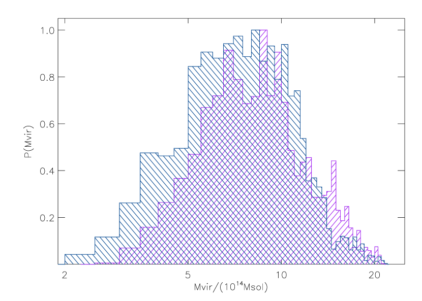
Figure 11: The probability density function of the Coma virial mass, derived through the sheet technique. The distribution coming from the sheet 2 is the blue one, slightly to the left. The violet slightly narrower distribution corresponds to the sheet 1. The best mass estimate based on these measurement is: $M_{\rm vir}=(9.2\pm\,2.4)\times\,10^{14}\rm M_{\odot}$.

In Fig. 11, we overplot the probability distributions for the virial mass of Coma, from the analysis of the two sheets. The two probability distributions are very similar. The mean value of the virial mass is $M_{\rm vir}=(9.7\pm\,3.6)\times\,10^{14}\rm M_{\odot}$ for the sheet 1 and $M_{\rm vir}=(8.7\pm\,3.3)\times\,10^{14}\rm M_{\odot}$ for the sheet 2. When applying equation (1), these values give a virial radius of $r_{\rm vir}=2.5\,$Mpc and $r_{\rm vir}=2.4\,$Mpc, respectively. The best mass estimate based on the combination of these measurements is: $M_{\rm vir}=(9.2\pm\,2.4)\times\,10^{14}\rm M_{\odot}$.

Our result is in good agreement with previous estimates of the Coma cluster mass. In Hughes (1989), they obtain a virial mass $M_{\rm vir}=(13\pm\,2)\times 10^{14}\,M_{\odot}$ from their X-ray study. From the galaxy kinematic analysis, Łokas & Mamon (2003) report a virial mass $M_{100}=(15\pm\,4.5)\times 10^{14}\,M_{\odot}$, corresponding to a density contrast $\Delta=100$, which is very close to our value. Geller et al. (1999) find a mass $M_{200}=15\,\times\,10^{14}\,M_{\odot}$, corresponding to a density contrast $\Delta=200$. The weak lensing mass estimate in Kubo et al. (2007) gives $M_{200}=2.7^{+3.6}_{-1.9}\,\times\,10^{15}\,M_{\odot}$.

The mean value for cosine of the orientation angle is ${\rm cos}(\alpha)=0.36\pm\,0.01$, corresponding to $\alpha=-1.2\pm 0.01$ rad, for the sheet 1 and ${\rm cos}(\alpha)=0.64\pm\,0.02$, corresponding to $\alpha=0.87\pm\,0.02$ rad, for the sheet 2. These results are affected by a statistical error of $50\%$ for the mass and $2.5\%$ for the angle, as discussed in Section 4.2.

The value obtained for the orientation $\alpha$ of a sheet corresponds to the mean angle of all the galaxies belonging to the sheet. By knowing $\alpha$, we can calculate the corresponding coordinate along the line of sight for all the galaxies, and therefore, we reconstruct the three dimensional map of the two structures, as shown in Fig. 12. The sheets we find are lying on two different planes.

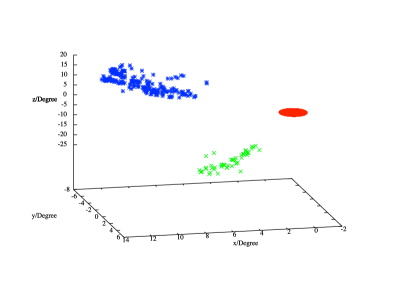
Figure 12: The sheets we found outside the Coma cluster in the three-dimensional space. The blue and the green points represent the particles belonging to the sheet 1 and the sheet 2, respectively. The Coma cluster is indicated as a red sphere centered at ($x,y,z$)=(0,0,0).

6 Summary and Conclusion

The main purpose of this paper is to propose and test a new method for the mass estimation of clusters within the virial radius. The idea is to infer it only from the kinematical data of structures in the cluster outskirts.

In the hierarchical scenario of structure formation, galaxy clusters are located at the intersection of filaments and sheets. The motion of such non-virialized structures is thus affected by the presence of the nearest massive cluster.

We found that modeling the kinematic data of these objects leads to an estimation of the neighbor cluster mass. The gravitational effect of the cluster mass is to perturb the pure Hubble motion, leading to a deceleration. Therefore, the measured departure from the Hubble flow of those structures allows us to infer the virial mass of the cluster. We have developed a technique to detect the presence of structures outside galaxy clusters, by looking at the velocity space. We underline that the proposed technique doesn’t aim to map all the objects around clusters, but it is limited to finding those structures that are suitable for the virial cluster mass estimation.

Our mass estimation method doesn’t require the dynamical analysis of the virialized region of the cluster, therefore it is not based on the dynamical equilibrium hypothesis. However, our method rely on the assumption of spherical symmetry of the system. In fact, we assume a radial velocity profile. Moreover, our method is biased by fixing the phenomenological fit to the radial infall velocity profile of simulation, as universal infall profile. From the practical point of view, this technique requires gathering galaxy positions and velocities in the outskirts of galaxy clusters, very far away from the cluster centre. A quite dense sample of redshifts is needed, in order to identify the possible presence of structures over the background. Once the structures are detected, the fit to their line of sight velocity profiles has to be performed. The fitting procedure involves only two free parameters: the virial mass of the cluster and the orientation angle of the structure in 3D. This makes the estimation of the virial cluster mass quite easy to obtain.

We have analysed cosmological simulations first, in order to test both the technique to identify structures outside clusters and the method to extract the cluster mass. We find one sheet outside the selected simulated halo, and we infer the correct halo mass and sheet orientation angle, within the errors.

We then applied our method to the Coma cluster. We have analysed the SDSS data of projected distances and velocities, up to $20\,$Mpc far from the Coma centre. Our work led to the detection of two galactic sheets in the environment of the Coma cluster. The estimation of the Coma cluster mass through the analysis of the two sheets, gives $M_{\rm vir}=(9.2\pm\,2.4)\times\,10^{14}\rm M_{\odot}$. This value is in agreement with previous results from the standard methods. We note however that our method tends to underestimate the Coma virial mass, compared with previous measurements, which either assume equilibrium or sphericity.

In the near future, we aim to apply our technique to other surveys, where redshifts at very large distances from the clusters centre are available. If a large number of sheets and filaments will be found, our method could also represent a tool to deproject the spatial distribution of galaxies outside galaxy clusters into the three-dimensional space.

7 Acknowledgements

The authors thank Stefan Gottloeber, who kindly agreed for one of the CLUES simulations (http://www.clues-project.org/simulations.html) to be used in the paper. The simulation has been performed at the Leibniz Rechenzentrum (LRZ), Munich. The Dark Cosmology Centre is funded by the Danish National Research Foundation.

References

- Abazajian et al. (2009) Abazajian K. N. et al., 2009, ApJs, 182, 543
- Allen et al. (2011) Allen S. W., Evrard A. E., Mantz A. B., 2011, Annual Review of Astronomy and Astrophysics, 49, 409
- Aragón-Calvo et al. (2007) Aragón-Calvo M. A., Jones B. J. T., van de Weygaert R., van der Hulst J. M., 2007, A&A, 474, 315
- Aragón-Calvo et al. (2010) Aragón-Calvo M. A., van de Weygaert R., Jones B. J. T., 2010, MNRAS, 408, 2163
- Biviano (1998) Biviano A., 1998, arXiv:astro-ph/9711251
- Bond et al. (1996) Bond J. R., Kofman L., Pogosyan D., 1996, Nature, 380, 603
- Bond et al. (2010) Bond N. A., Strauss M. A., Cen R., 2010, MNRAS, 409, 156
- Borgani et al. (2004) Borgani S. et al., 2004, MNRAS, 348, 1078
- Brinckmann et al. (2013) Brinckmann T., Lindholmer M., Falco M., Hansen S. H., Wojtak R., Sparre M., 2013, in preparation
- Colberg et al. (2005) Colberg J. M., Krughoff K. S., Connolly A. J., 2005, MNRAS, 359, 272
- Colberg et al. (1999) Colberg J. M., White S. D. M., Jenkins A., Pearce F. R., 1999, MNRAS, 308, 593
- Colless et al. (2003) Colless M. et al., 2003, VizieR Online Data Catalog, 7226
- Cuesta et al. (2008) Cuesta A. J., Prada F., Klypin A., Moles M., 2008, MNRAS, 389, 385
- Cunha et al. (2009) Cunha C., Huterer D., Frieman J. A., 2009, Phys. Rev. D, 80, 063532
- Davis et al. (1985) Davis M., Efstathiou G., Frenk C. S., White S. D. M., 1985, ApJ, 292, 371
- de Lapparent et al. (1986) de Lapparent V., Geller M. J., Huchra J. P., 1986, ApJL, 302
- Diaferio (1999) Diaferio A., 1999, MNRAS, 309, 610
- Dietrich et al. (2012) Dietrich J. P., Werner N., Clowe D., Finoguenov A., Kitching T., Miller L., Simionescu A., 2012, Nature, 487, 202
- Einasto et al. (1984) Einasto J., Klypin A. A., Saar E., Shandarin S. F., 1984, MNRAS, 206, 529
- Ettori et al. (2002) Ettori S., Fabian A. C., Allen S. W., Johnstone R. M., 2002, MNRAS, 331, 635
- Falco et al. (2013) Falco M., Mamon G. A., Wojtak R., Hansen S. H., Gottlöber S., 2013, arXiv:astro-ph/1306.6637
- Gavazzi et al. (2009) Gavazzi R., Adami C., Durret F., Cuillandre J.-C., Ilbert O., Mazure A., Pelló R., Ulmer M. P., 2009, Astronomy and Astrophysics, 498, L33
- Geller et al. (1999) Geller M. J., Diaferio A., Kurtz M. J., 1999, ApJL, 517, L23
- Geller & Huchra (1989) Geller M. J., Huchra J. P., 1989, Science, 246, 897
- Girardi et al. (1998) Girardi M., Giuricin G., Mardirossian F., Mezzetti M., Boschin W., 1998, ApJ, 505, 74
- Gottloeber & Klypin (2008) Gottloeber S., Klypin A., 2008, arXiv:0803.4343
- Gregory et al. (1978) Gregory S. A., Thompson L. A., Tifft W. G., 1978, Bulletin of the American Astronomical Society, 10, 622
- Hahn et al. (2007) Hahn O., Porciani C., Carollo C. M., Dekel A., 2007, MNRAS, 375, 489
- Haiman et al. (2001) Haiman Z., Mohr J. J., Holder G. P., 2001, ApJ, 553, 545
- Hoffman et al. (2012) Hoffman Y., Metuki O., Yepes G., Gottlöber S., Forero-Romero J. E., Libeskind N. I., Knebe A., 2012, MNRAS, 425, 2049
- Host & Hansen (2011) Host O., Hansen S. H., 2011, ApJ, 736, 52
- Huchra et al. (2005) Huchra J. et al., 2005, Astronomical Society of the Pacific Conference Series, 329, 135
- Hughes (1989) Hughes J. P., 1989, ApJ, 337, 21
- Karachentsev & Nasonova (2010) (Kashibadze) Karachentsev I. D., Nasonova (Kashibadze) O. G., 2010, Astrophysics, 53, 32
- Kent & Gunn (1982) Kent S. M., Gunn J. E., 1982, AJ, 87, 945
- Kravtsov et al. (1997) Kravtsov A. V., Klypin A. A., Khokhlov A. M., 1997, ApJs, 111, 73
- Kubo et al. (2007) Kubo J. M., Stebbins A., Annis J., Dell’Antonio I. P., Lin H., Khiabanian H., Frieman J. A., 2007, ApJ, 671, 1466
- Łokas & Mamon (2003) Łokas E. L., Mamon G. A., 2003, MNRAS, 343, 401
- Łokas et al. (2006) Łokas E. L., Wojtak R., Gottlöber S., Mamon G. A., Prada F., 2006, MNRAS, 367, 1463
- Lombriser (2011) Lombriser L., 2011, Phys. Rev. D,, 83, 063519
- Mamon & Boué (2010) Mamon G. A., Boué G., 2010, MNRAS, 401, 2433
- Mamon et al. (2004) Mamon G. A., Sanchis T., Salvador-Solé E., Solanes J. M., 2004, A&A, 414, 445
- Mandelbaum et al. (2010) Mandelbaum R., Seljak U., Baldauf T., Smith R. E., 2010, MNRAS, 405, 2078
- Nasonova et al. (2011) Nasonova O. G., de Freitas Pacheco J. A., Karachentsev I. D., 2011, A&A, 532, A104
- Novikov et al. (2006) Novikov D., Colombi S., Doré O., 2006, MNRAS, 366, 1201
- Peebles (1980) Peebles P. J. E., 1980, The large-scale structure of the universe. Research supported by the National Science Foundation. Princeton, N.J., Princeton University Press, 1980. 435 p.
- Peirani & de Freitas Pacheco (2006) Peirani S., de Freitas Pacheco J. A., 2006, New Astronomy, 11, 325
- Peirani & de Freitas Pacheco (2008) Peirani S., de Freitas Pacheco J. A., 2008, A&A, 488, 845
- Porter et al. (2008) Porter S. C., Raychaudhury S., Pimbblet K. A., Drinkwater M. J., 2008, MNRAS, 388, 1152
- Prada et al. (2006) Prada F., Klypin A. A., Simonneau E., Betancort-Rijo J., Patiri S., Gottlöber S., Sanchez-Conde M. A., 2006, ApJ, 645, 1001
- Rines & Diaferio (2006) Rines K., Diaferio A., 2006, The Astronomical Journal, 132, 1275
- Schmidt & Allen (2007) Schmidt R. W., Allen S. W., 2007, MNRAS, 379, 209
- Shandarin & Zeldovich (1983) Shandarin S. F., Zeldovich I. B., 1983, Comments on Astrophysics, 10, 33
- Shectman et al. (1996) Shectman S. A., Landy S. D., Oemler A., Tucker D. L., Lin H., Kirshner R. P., Schechter P. L., 1996, ApJ, 470, 172
- Sousbie et al. (2008) Sousbie T., Pichon C., Colombi S., Novikov D., Pogosyan D., 2008, MNRAS, 383, 1655
- Sparre (2013) Sparre M., 2013, submitted to JCAP
- Tegmark et al. (2004) Tegmark M. et al., 2004, ApJ, 606, 702
- The & White (1986) The L. S., White S. D. M., 1986, Astronomical Journal, 92, 1248
- van de Weygaert & Bond (2008) van de Weygaert R., Bond J. R., 2008, Lecture Notes in Physics, Berlin Springer Verlag, 740, 409
- van Haarlem & van de Weygaert (1993) van Haarlem M., van de Weygaert R., 1993, ApJ, 418, 544
- Wadekar & Hansen (2013) Wadekar D., Hansen S. H., 2013, in preparation
- Watt et al. (1992) Watt M. P., Ponman T. J., Bertram D., Eyles C. J., Skinner G. K., Willmore A. P., 1992, MNRAS, 258, 738
- White et al. (2010) White M., Cohn J. D., Smit R., 2010, MNRAS, 408, 1818
- White & Frenk (1991) White S. D. M., Frenk C. S., 1991, ApJ, 379, 52
- Wojtak et al. (2005) Wojtak R., Łokas E. L., Gottlöber S., Mamon G. A., 2005, MNRAS, 361, L1
- Wojtak et al. (2008) Wojtak R., Łokas E. L., Mamon G. A., Gottlöber S., Klypin A., Hoffman Y., 2008, MNRAS, 388, 815
- Zappacosta et al. (2006) Zappacosta L., Buote D. A., Gastaldello F., Humphrey P. J., Bullock J., Brighenti F., Mathews W., 2006, ApJ, 650, 777
- Zeldovich et al. (1982) Zeldovich I. B., Einasto J., Shandarin S. F., 1982, Nature, 300, 407
- Zwicky (1933) Zwicky F., 1933, Helvetica Physica Acta, 6, 110