Cumulants associated with geometric phases

Abstract

The Berry phase can be obtained by taking the continuous limit of a cyclic product $-\mbox{Im}\ln\prod_{I=0}^{M-1}\langle\Psi_{0}({\bm{\xi}}_{I})|\Psi_{0}({\bm{\xi}}_{I+1})\rangle$, resulting in the circuit integral $i\oint\mbox{d}{\bm{\xi}}\cdot\langle\Psi_{0}({\bm{\xi}})|\nabla_{\bm{\xi}}|\Psi_{0}({\bm{\xi}}\rangle$. Considering a parametrized curve ${\bm{\xi}}(\chi)$ we show that the product $\prod_{I=0}^{M-1}\langle\Psi_{0}(\chi_{I})|\Psi_{0}(\chi_{I+1})\rangle$ can be equated to a cumulant expansion. The first contributing term of this expansion is the Berry phase itself, the other terms are the associated spread, skew, kurtosis, etc. The cumulants are shown to be gauge invariant. It is also shown that these quantities can be expressed in terms of an operator.

Introduction. The concept of geometric phase was first suggested by Pancharatnam Pancharatnam56 in optics. In 1984 Berry Berry84 published a paper about phases which arise when a quantum system is brought around an adiabatic cycle. The phase advocated in this paper was overlooked earlier Fock28 as it was considered part of the arbitrary phase of a quantum wavefunction. Berry has shown that this is not the case, and that the phase of an adiabatic cycle can be a measurable quantity. Since the publication of Berry’s paper this concept was found to be at the core Shapere89 ; Xiao10 of a number of interesting physical effects, including the Aharonov-Bohm effect Aharonov59 , quantum Hall effect Thouless82 , topological insulators Hasan10 , dc conductivity Hetenyi13 , or the modern theory of polarization King-Smith93 ; Resta94 . More recently an example of a geometric phase, the Zak phase, has been measured in optical waveguidesLonghi13 and optical lattices Atala13 .

To derive a Berry phase, one considers a Hamiltonian which depends parametrically on a set of variables. One can then take a discrete set of points in this parameter space, obtain the wavefunction, and form a cyclic product of the type in Eq. (2). The imaginary part of the logarithm of this cyclic product corresponds to the discrete Berry phase. If the discrete points are along a cyclic curve then the continuous limit can be taken, and it corresponds to the well-known circuit integral Berry84 . The real part of the product is usually not considered, due to the common belief that as a result of the normalization of the wave-function, it is zero, therefore not physically relevant. In this paper we consider a curve parametrized by a scalar and show that when the real part of the product in Eq. (2) is considered it leads to a physically well-defined quantity. More generally we show that the product in Eq. (2) can be expanded using the standard cumulant expression, with the first order term corresponding to the Berry phase, and the higher order terms giving gauge invariant and therefore physically well-defined quantities. It is also shown that the cumulants can be written in terms of an operator. We then consider the spread of polarization, which was given by Resta and Sorella Resta99 , and show that the spread suggested by them coincides with that obtained from the cumulant expansion described here. We also analyze one of the canonical examples for the Berry phase Berry84 in light of our findings.

General remarks. The most general way to obtain the Berry phase is to write it in the discrete representation, and then take the continuous limit. Pancharatnam’s Pancharatnam56 original derivation is based on considering discrete phase changes. The discrete Berry phase first appeared in 1964, in a paper by Bargmann Bargmann64 , as a mathematical tool for proving a theorem. The expression which forms the basis of our derivation here has also been used extensively in the case of path-integral based representation of geometric phases Kuratsuji85 ; Kuratsuji86 .

Given a parameter space ${\bm{\xi}}$ and some Hamiltonian $H({\bm{\xi}})$ with

$$H({\bm{\xi}})|\Psi_{i}({\bm{\xi}})\rangle=E_{i}({\bm{\xi}})|\Psi_{i}({\bm{\xi}})\rangle,$$ (1)

where $|\Psi_{i}({\bm{\xi}})\rangle$($E_{i}({\bm{\xi}})$) is an eigenstate(eigenvalue) of the Hamiltonian. Consider a set of $M$ points in this parameter space $\{{\bm{\xi}}_{I}\}$. In this case one can form the quantity

$$\phi=-\mbox{Im}\ln\prod_{I=0}^{M-1}\langle\Psi_{0}({\bm{\xi}}_{I})|\Psi_{0}({\bm{\xi}}_{I+1})\rangle,$$ (2)

where $\Psi_{0}({\bm{\xi}}_{M})=\Psi_{0}({\bm{\xi}}_{0})$ (cyclic) which is physically well-defined since arbitrary phases cancel. In Eq. (2) $\phi$ is formed using the ground state, without loss of generality. If the points $\{{\bm{\xi}}_{I}\}$ are points on a closed curve, one can take the continuous limit and obtain

$$\phi=i\oint\mbox{d}{\bm{\xi}}\cdot\langle\Psi_{0}({\bm{\xi}})|\nabla_{\bm{\xi}}|\Psi_{0}({\bm{\xi}}\rangle.$$ (3)

The $\phi$ can be shown to be gauge invariant and is therefore a physically well-defined quantity. If the wavefunction can be taken to be real, then a nontrivial Berry phase corresponds to $\phi=\pi$ and will only occur if the enclosed region of parameter space is not simply connected. If the wavefunctions can not be taken as real then a non-trivial Berry phase can occur even if the parameter space is not simply connected.

Cumulant expansion of the Bargmann invariant. We consider the product in Eq. (2) along a cyclic curve. We assume that the curve is parametrized according to a scalar hence the product is $\prod_{I=0}^{M-1}\langle\Psi_{0}(\chi_{I})|\Psi_{0}(\chi_{I+1})\rangle$. We also assume that the length of the curve is $\Lambda$ and that $\chi_{I}$ defines an evenly spaced (spacing $\Delta\chi$) grid. We start by equating this product to a cumulant expansion,

$$\prod_{I=0}^{M-1}\langle\Psi_{0}(\chi_{I})|\Psi_{0}(\chi_{I+1})\rangle=\exp\left(\frac{1}{\Delta\chi}\sum_{n=1}^{\infty}\frac{(i\Delta\chi)^{n}}{n!}C_{n}\right).$$ (4)

Straightforward algebra and taking the continuous limit ($\Delta\chi\rightarrow 0$, $M\rightarrow\infty$, $\Lambda$ fixed) gives

$$C_{1} = -i\int_{0}^{\Lambda}d\chi\gamma_{1}$$ (5)

$$C_{2} = -\int_{0}^{\Lambda}d\chi[\gamma_{2}-\gamma_{1}^{2}]$$

$$C_{3} = i\int_{0}^{\Lambda}d\chi[\gamma_{3}-3\gamma_{2}\gamma_{1}+2\gamma_{1}^{3}]$$

$$C_{4} = \int_{0}^{\Lambda}d\chi[\gamma_{4}-3\gamma_{2}^{2}-4\gamma_{3}\gamma_{1}+12\gamma_{1}^{2}\gamma_{2}-6\gamma_{1}^{4}]$$

with $\gamma_{i}=\langle\Psi_{0}(\chi)|\partial^{i}_{\chi}|\Psi_{0}(\chi)\rangle$.

$C_{1}$ corresponds to the Berry phase. The other $C_{i}$ look very similar to the usual cumulants (compare coefficients), provided that we can interpret $-i\partial_{\chi}$ as an operator and the integral as an expectation value. $C_{1}$ is known to be gauge invariant, therefore it is natural to ask whether the other $C_{i}$ are also gauge invariant. We consider the proof of gauge invariance for $C_{1}$. One first alters the phase of the wavefunction, i.e. define

$$|\tilde{\Psi}_{0}(\chi)\rangle=\exp[i\beta(\chi)]|\Psi_{0}(\chi)\rangle.$$ (6)

Defining

$$\tilde{C}_{1}=-i\int_{0}^{\Lambda}d\chi\langle\tilde{\Psi}_{0}(\chi)|\partial_{\chi}|\tilde{\Psi}_{0}(\chi)\rangle,$$ (7)

it is easy to show that

$$\tilde{C}_{1}-C_{1}=\beta(\Lambda)-\beta(0).$$ (8)

with $\tilde{\gamma}_{1}=\langle\tilde{\Psi_{0}}(\chi)|\partial^{i}_{\chi}|\tilde{\Psi_{0}}(\chi)\rangle$. Hence the Berry phase of the original wavefunction differs from the shifted one by the difference of $\beta(\Lambda)-\beta(0)$ which for an adiabatic cycle is $2\pi m$, with $m$ integer. Applying the same procedure to the other cumulants we obtain the following results:

$$\tilde{C}_{2}-C_{2} = \dot{\beta}(\Lambda)-\dot{\beta}(0)=0,$$ (9)

$$\tilde{C}_{3}-C_{3} = \ddot{\beta}(\Lambda)-\ddot{\beta}(0)=0,$$

$$\tilde{C}_{4}-C_{4} = \dddot{\beta}(\Lambda)-\dddot{\beta}(0)=0,$$

hence, if the function $\beta(\chi)$ and its derivatives are continuous at the boundaries gauge invariance holds. We have carried out this proof up to fourth order. There appears to be a pattern in Eq. (9).

The cumulants derived above can be expressed in terms of expectation values of operators. Consider the expression from perturbation theory

$$\partial_{\chi}|\Psi_{0}(\chi)\rangle=\sum_{j\neq 0}|\Psi_{j}(\chi)\rangle\langle\Psi_{j}(\chi)|\frac{\partial_{\chi}H(\chi)}{E_{j}-E_{0}}|\Psi_{0}(\chi)\rangle.$$ (10)

Defining operator $\hat{O}$ as

$$\partial_{\chi}H(\chi)=i[H(\chi),\hat{O}]$$ (11)

it can be shown that the cumulants of this operator correspond to the $C_{i}$ derived above, except for the case $i=1$, the Berry phase itself, for which application of Eq. (10) leads to zero. For the Berry phase the expression from perturbation theory (Eq. (10 )) is not valid since it makes a definite choice about the phase of the wavefunction for all values of $\chi$. The most general expression is

$$|\Psi(\chi+\Delta\chi)\rangle=e^{i\alpha}\times\hskip 85.35826pt$$ (12)

$$\left[|\Psi(\chi)\rangle+\sum_{j\neq 0}|\Psi_{j}(\chi)\rangle\langle\Psi_{j}(\chi)|\frac{\partial_{\chi}H(\chi)}{E_{j}-E_{0}}|\Psi_{0}(\chi)\rangle\right],$$

but in standard perturbation theory $\alpha$ is assumed to be zero. This phase difference shifts the first cumulant (the Berry phase), however since it is a mere shift, it leaves the other cumulants unaffected. One can conclude that while the Berry phase itself can not be expressed in terms of an operator, its associated cumulants can. This statement will be clarified in an example below.

Polarization, current and their spreads. We now consider the Berry phase corresponding to the polarization from the modern theory King-Smith93 ; Resta94 ; Resta99 ; Resta98 . In this theory an expression for the spread of a Berry phase associated quantity has been suggested, and we now show that it is equivalent to $C_{2}/\Lambda$.

Resta showed that the expectation value of the position over some wavefunction $|\Psi_{0}\rangle$ of a system with unit cell dimension $L$ can be written as

$$\langle X\rangle=-\frac{1}{\Delta K}\mbox{Im}\ln\langle\Psi_{0}|e^{-i\Delta K\hat{X}}|\Psi_{0}\rangle,$$ (13)

where $\Delta K=2\pi/(N_{k}L)$, $N_{k}$ denotes an integer, $\hat{X}=\sum_{j}\hat{x}_{j}$ is the sum of the positions of all particles. The spread in position ($\sigma^{2}_{X}=\langle X^{2}\rangle-\langle X\rangle^{2}$) can be written

$$\sigma^{2}_{X}=-\frac{2}{\Delta K^{2}}\mbox{Re}\ln\langle\Psi_{0}|e^{-i\Delta K\hat{X}}|\Psi_{0}\rangle,$$ (14)

The operator $e^{i\Delta K\hat{X}}$ is the total momentum shift operator which, as has been shown elsewhere Hetenyi09 ; Essler05 has the property that for a state $|\Psi_{0}(K)\rangle$ with particular crystal momentum $K$ defined as

$$\Psi_{0}(k_{1}+K,k_{2}+K,...),$$ (15)

it holds that

$$e^{-i\Delta K\hat{X}}|\Psi_{0}(K)\rangle=|\Psi_{0}(K+\Delta K)\rangle,$$ (16)

in other words it shifts the crystal momentum by $\Delta K$. To use the shift operator we first write

$$\sigma^{2}_{X}=-\frac{2}{N_{k}\Delta K^{2}}\mbox{Re}\ln\langle\Psi_{0}|e^{-i\Delta K\hat{X}}|\Psi_{0}\rangle^{N_{k}}.$$ (17)

We associate the state $|\Psi_{0}\rangle$ with a particular crystal momentum $K_{0}$,

$$|\Psi_{0}\rangle=|\Psi_{0}(K_{0})\rangle.$$ (18)

Using the total momentum shift the scalar product can be rewritten as

$$\langle\Psi_{0}(K_{0})|e^{-i\Delta K\hat{X}}|\Psi_{0}(K_{0})\rangle = \langle\Psi_{0}(K_{0})|\Psi_{0}(K_{1})\rangle$$ (19)

$$= \langle\Psi_{0}(K_{I})|\Psi_{0}(K_{I+1})\rangle,$$

where $K_{I+1}=K_{I}+\Delta K$. To show the last equation one applies the Hermitian conjugate of the total momentum shift to $\langle\Psi_{0}(K_{0})|$ $I$ times and the total momentum shift operator to $|\Psi_{0}(K_{0})\rangle$ $I+1$ times and forms the scalar product. Thus we can also write

$$\langle\Psi_{0}(K_{0})|e^{-i\Delta K\hat{X}}|\Psi_{0}(K_{0})\rangle^{N_{k}}=\prod_{I=0}^{N_{k}-1}\langle\Psi_{0}(K_{I})|\Psi_{0}(K_{I+1})\rangle.$$ (20)

The points $K_{I}$ form an evenly spaced grid with spacing $\Delta K$ in the Brillouin zone. Using this result the spread can be rewritten as

$$\sigma^{2}_{X}=-\frac{2}{N_{k}\Delta K^{2}}\sum_{I=0}^{N_{k}}\mbox{Re}\ln\langle\Psi_{0}(K_{I})|\Psi_{0}(K_{I+1})\rangle,$$ (21)

We now expand the scalar product up to second order as

$$\langle\Psi_{0}(K_{I})|\Psi_{0}(K_{I+1})\rangle=1+\Delta K\langle\Psi_{0}(K_{I})|\partial_{K}|\Psi_{0}(K_{I})\rangle+$$

$$\frac{\Delta K^{2}}{2}\langle\Psi_{0}(K_{I})|\partial^{2}_{K}|\Psi_{0}(K_{I})\rangle.\hskip 28.45274pt$$ (22)

Subsequent expansion of the logarithm and keeping all terms up to second order in $\Delta K$ results in a first order term of the form

$$\frac{N_{k}L^{2}}{2\pi^{2}}\mbox{Re}\sum_{I=0}^{N_{k}-1}\Delta K\langle\Psi_{0}(K_{I})|\partial_{K}|\Psi_{0}(K_{I})\rangle.$$ (23)

In the continuum limit ($N_{k}\rightarrow\infty$) the sum turns into the integral which gives the standard Berry phase, but since this integral is purely imaginary it will not contribute to the spread. The final result for the spread is

$$\sigma^{2}_{X}=\frac{L}{2\pi}\sum_{I=0}^{N_{k}-1}\Delta K\sigma^{2}_{X}(K_{I})=\frac{L}{2\pi}\int_{-\pi/L}^{\pi/L}\mbox{d}K\sigma^{2}_{X}(K),$$ (24)

where

$$\sigma^{2}_{X}(K)=-\langle\Psi_{0}(K)|\partial^{2}_{K}|\Psi_{0}(K)\rangle+\langle\Psi_{0}(K)|\partial_{K}|\Psi_{0}(K)\rangle^{2}.$$ (25)

Eq. (24) is actually the average of the spread over the Brillouin zone. One can think of $i\partial_{K}$ as a “heuristic position operator” Vanderbilt06 , and the quantity $\sigma^{2}_{X}(K)$ as the spread for a wavefunction with crystal momentum $K$. This spread of the position operator, derived by different means, has also been obtained by Marzari and Vanderbilt Marzari97 . One can also start from the expression for the spread of the total current Hetenyi12b

$$\sigma^{2}_{K}=-\frac{2}{\Delta X^{2}}\mbox{Re}\ln\langle\Psi_{0}|e^{-i\Delta X\hat{K}}|\Psi_{0}\rangle,$$ (26)

and apply exactly the same steps as in the case of the total position. This derivation results in

$$\sigma^{2}_{K}=-\frac{1}{L}\int_{0}^{L}\mbox{d}X[\langle\Psi_{0}(X)|\partial^{2}_{X}|\Psi_{0}(X)\rangle-\langle\Psi_{0}(X)|\partial_{X}|\Psi_{0}(X)\rangle^{2}].$$ (27)

Example. We now calculate the cumulants up to fourth order for one of the canonical examples for the Berry phase Berry84 , a spin-$\frac{1}{2}$ particle in a precessing magnetic field. The Hamiltonian is given by

$$\hat{H}(t)=-\mu{\bf B}(t)\cdot{\bm{\sigma}},$$ (28)

where ${\bm{\sigma}}$ are the Pauli matrices, and ${\bf B}(t)$ denotes the magnetic field,

$${\bf B}(t)=\left[\begin{array}[]{c}\sin\theta\cos\phi\\ \sin\theta\sin\phi\\ \cos\theta\end{array}\right].$$ (29)

The $z$-component of the field is fixed, the projection on the $x-y$-plane is performing rotation, i.e. $\phi=\omega t$. We can proceed to evaluate the Berry phase and the associated cumulants by defining an adiabatic cycle in which $\phi$ rotates from zero to $2\pi$. Using one of the eigenstates

$$|n_{-}(t)\rangle=\left[\begin{array}[]{c}-\sin\left(\frac{\theta}{2}\right)\\ e^{i\phi}\cos\left(\frac{\theta}{2}\right)\end{array}\right].$$ (30)

The associated cumulants (divided by $2\pi$) evaluate to

$$C_{1}= \cos^{2}\left(\frac{\theta}{2}\right),$$ (31)

$$C_{2}= \left[\cos^{2}\left(\frac{\theta}{2}\right)-\cos^{4}\left(\frac{\theta}{2}\right)\right],$$

$$C_{3}= \left[\cos^{2}\left(\frac{\theta}{2}\right)-3\cos^{4}\left(\frac{\theta}{2}\right)+2\cos^{6}\left(\frac{\theta}{2}\right)\right],$$

$$C_{4}= \left[\cos^{2}\left(\frac{\theta}{2}\right)-7\cos^{4}\left(\frac{\theta}{2}\right)+12\cos^{6}\left(\frac{\theta}{2}\right)-6\cos^{8}\left(\frac{\theta}{2}\right)\right].$$

Fig. 1 shows the cumulants as a function of the angle $\theta$. $C_{1}$, the Berry phase associated with a spin$-\frac{1}{2}$ particle in a precessing magnetic field is a well-known result. The spread is zero when the Berry phase is zero or $\pi$. The skew changes sign halfway between zero and $\pi$ and the kurtosis also varies in sign as a function of the angle $\theta$.

The operator $\hat{O}$ for this example can easily be shown to be the Pauli matrix $\frac{\sigma_{z}}{2}$. The first order cumulant is given by

$$\left\langle\frac{\sigma_{z}}{2}\right\rangle=\sin^{2}\left(\frac{\theta}{2}\right)-\cos^{2}\left(\frac{\theta}{2}\right).$$ (32)

in other words it is merely shifted compared to the Berry phase. The higher order cumulants are identical to those in Eqs. (31). In the operator representation of the Berry phase the meaning of the first and second cumulants is rendered more clear. For the value of $\theta$ for which $\langle\sigma_{z}/2\rangle$ is either $\pm\frac{1}{2}$ the spread is zero. Indeed those are the maximum and minimum values the operator $\sigma_{z}$ can take, hence the spread must be zero. It is obvious from these results that the cumulants derived from the Bargmann invariant give information about the probability distribution of the operator associated with the Berry phase.

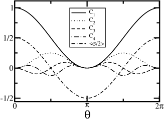
Figure 1: Cumulants of a spin$-\frac{1}{2}$ particle in a precessing field.

Measurement of $C_{i}$s. While it has been shown that $C_{i}$ are physically well-defined their measurement may not be trivial. The operator may not exist or be easily written down. In this case one can proceed as follows. Define:

$${\bm{\Pi}} = \prod_{I=0}^{M-1}\langle\Psi_{0}(\chi_{I})|\Psi_{0}(\chi_{I+1})\rangle,$$ (33)

$${\bm{\Pi}}^{(o)} = \prod_{I=0}^{M/2-1}\langle\Psi_{0}(\chi_{2I+1})|\Psi_{0}(\chi_{2I+3})\rangle,$$

$${\bm{\Pi}}^{(e)} = \prod_{I=0}^{M/2-1}\langle\Psi_{0}(\chi_{2I})|\Psi_{0}(\chi_{2I+2})\rangle.$$

Using these definitions one can show that

$$C_{3} \approx \frac{2}{\Delta\chi^{2}}\mbox{Im}\ln\left[\frac{({\bm{\Pi}}^{(o)}{\bm{\Pi}}^{(e)})^{\frac{1}{2}}}{{\bm{\Pi}}}\right]+O(\Delta\chi^{3}),$$ (34)

$$C_{4} \approx \frac{4}{\Delta\chi^{3}}\mbox{Re}\ln\left[\frac{({\bm{\Pi}}^{(o)}{\bm{\Pi}}^{(e)})^{\frac{1}{4}}}{{\bm{\Pi}}}\right]+O(\Delta\chi^{3}).$$

Conclusions. In this paper it was shown that there exists a cumulant expansion associated with the Berry phase. The starting point was the Bargmann invariant, which gives rise to the discrete Berry phase. The Bargmann invariant was expressed in terms of a cumulant expansion, the first term of which was shown to correspond to the Berry phase. Up to fourth order it was demonstrated that the cumulants are gauge invariant. It was also shown that the cumulants derived can also be related to corresponding expectation values of a particular operator. Since, in the modern theory of polarization, an expression for the second cumulant (spread or variance) is already in use, as a consistency check, equivalence between that and the spread resulting from the cumulant expansion presented here was shown. The cumulants were calculated for a simple example.

Acknowledgments. BH acknowledges a grant from the Turkish agency for basic research (TÜBITAK, grant no. 112T176).

References

• (1) S. Pancharatnam, Proc. Indian Acad. Sci. A 44 247 (1956).
• (2) M. V. Berry, Proc. Roy. Soc. London A392 45 (1984).
• (3) V. Fock, Z. Phys. 49 323 (1928).
• (4) A. Shapere and F. Wilczek, Geometric Phases in Physics, World Scientific, (1989).
• (5) D. Xiao, M.-C. Chang, and Q. Niu, Rev. Mod. Phys. 82 1959 (2010).
• (6) Y. Aharonov and D. Bohm, Phys. Rev. 115 485 (1959).
• (7) D. J. Thouless, M. Kohmoto, M. P. Nightingale, and M. den Nijs Phys. Rev. Lett 49 405 (1982).
• (8) M. Z. Hasan and C. L. Kane, Rev. Mod. Phys. 82 3045 (2010).
• (9) B. Hetényi, Phys. Rev. B 87 235123 (2013).
• (10) R. D. King-Smith and D. Vanderbilt, Phys. Rev. B 47 1651 (1993).
• (11) R. Resta, Rev. Mod. Phys. 66 899 (1994).
• (12) S. Longhi, Opt. Lett. 38 3716 (2013).
• (13) M. Atala, M. Aidelsburger, J. T. Barreiro, D. Abanin, T. Kitagawa, E. Demmler, and I. Bloch, Nature (2013).
• (14) H. Kuratsuji, Phys. Lett. A 120 141 (1987).
• (15) J. Zak, Phys. Rev. 62 2747 (1989).
• (16) R. Resta and S. Sorella, Phys. Rev. Lett. 82 370 (1999).
• (17) A. Selloni, P. Carnevali, R. Car and M. Parrinello, Phys. Rev. Lett., 59 823 (1987).
• (18) E. S. Fois, A. Selloni, M. Parrinello and R. Car, J. Phys. Chem., 92 3268 (1988).
• (19) R. Resta, Phys. Rev. Lett. 80 1800 (1998).
• (20) V. Bargmann J. Math. Phys. 5 862 (1964).
• (21) H. Kuratsuji and S. Iida Prog. Theor. Phys. 74 439 (1985).
• (22) H. Kuratsuji and S. Iida Phys. Rev. Lett. 56 1003 (1986).
• (23) B. Hetényi, J. Phys. A, 42 412003 (2009).
• (24) F. H. L. Essler, H. Frahm, F. Göhmann, A. Klümper, and V. E. Korepin, The One-Dimensional Hubbard Model, Cambridge University Press, (2005).
• (25) D. Vanderbilt and R. Resta, in Contemporary Concepts of Condensed Matter Science Chapter 5, pp. 139, Elsevier, (2006).
• (26) N. Marzari, and D. Vanderbilt, Phys. Rev. B 56 12847 (1997).
• (27) B. Hetényi, J. Phys. Soc. Japan 81 124711 (2012).