UWThPh-2013-19
CFTP/13-020
Double seesaw mechanism and lepton mixing

Abstract

We present a general framework for models in which the lepton mixing matrix is the product of the maximal mixing matrix $U_{\omega}$ times a matrix constrained by a well-defined $\mathbbm{Z}_{2}$ symmetry. Our framework relies on neither supersymmetry nor non-renormalizable Lagrangians nor higher dimensions; it relies instead on the double seesaw mechanism and on the soft breaking of symmetries. The framework may be used to construct models for virtually all the lepton mixing matrices of the type mentioned above which have been proposed in the literature.

1 Introduction

With the measurement of the reactor mixing angle $\theta_{13}$ [1], our knowledge of the lepton mixing matrix $U$ is almost complete. Only the CKM-type phase $\delta$ is still unknown. Because $s_{13}^{2}$ ($s_{ij}\equiv\sin\theta_{ij}$ and $c_{ij}\equiv\cos\theta_{ij}$ for $i,j=1,2,3$) is definitely nonzero, strict tri-bimaximal mixing (TBM) [3] is ruled out. However, it is still viable to relax TBM in such a way that either the first column ($u_{1}$) or the second column ($u_{2}$) of $U=\left(u_{1},\,u_{2},\,u_{3}\right)$ coincides with its form in TBM. Let TM₁ and TM₂, respectively, denote these two possibilities [4]. In a suitable phase convention, one has

$$\mbox{TM}_{1}: u_{1}=\frac{1}{\sqrt{6}}\left(\begin{array}[]{c}2\\ -1\\ -1\end{array}\right),$$ (1d)

$$\mbox{TM}_{2}: u_{2}=\frac{1}{\sqrt{3}}\left(\begin{array}[]{c}1\\ 1\\ 1\end{array}\right).$$ (1h)

On the other hand, many authors [5] have recently pursued an approach in which $U$ is either partially or completely determined by distinct symmetries in the charged-lepton mass matrix $M_{\ell}$ and in the light-neutrino Majorana mass matrix $M_{\nu}$. Those distinct symmetries are conceived as remnants of the full flavour symmetry group of the Lagrangian. In particular, in ref. [6] three candidates for a completely determined $U$ have been found in this way. In that approach, $U$ can be written, in the weak basis in which the models are formulated, as the product

$$U=U_{\omega}V,$$ (2)

where

$$U_{\omega}\equiv\frac{1}{\sqrt{3}}\left(\begin{array}[]{ccc}1&1&1\\ 1&\omega&\omega^{2}\\ 1&\omega^{2}&\omega\end{array}\right)$$ (3)

($\omega\equiv\exp{\left(2\pi i/3\right)}$) is a symmetric unitary matrix, which diagonalizes $M_{\ell}$ in that weak basis, while $V$ is the unitary matrix that diagonalizes $M_{\nu}$. In this approach the matrix $V$ is constrained by either one or two well-defined $\mathbbm{Z}_{2}$ symmetries, leading to the determination of either one column or all the columns of $U$, respectively.

Unfortunately, it is not easy to implement the approach of the previous paragraph in the context of well-defined, self-contained models. The same happens if one tries to implement TM₁ in such models. One usually has recourse to supersymmetry, non-renormalizable Lagrangians, and additional superfields (‘familons’ and ‘driving fields’), or else to theories with extra dimensions; the resulting models tend to be complicated and unaesthetic.

In this paper we present a framework which allows one to realize, in a technically natural way, mixing matrices with either TM₁, TM₂, or virtually any of the viable mixing matrices found in refs. [5, 6]. Our framework relies on the double seesaw mechanism and on a soft flavour symmetry breaking in the Majorana mass matrix of right-handed neutrino singlets; it involves neither of the technical complications mentioned in the previous paragraph. On the other hand, our framework rests on two assumptions about the vacuum, which is characterized by two vastly different scales: the vacuum must preserve a symmetry of the Lagrangian at the high scale and break another symmetry of the Lagrangian at the low scale. Actually, it should be possible to implement these two assumptions by choosing suitable ranges for the parameters in the scalar potential. Unfortunately, we have been unable to prove this in all generality and beyond doubt.

Let us first discuss the double seesaw mechanism [9]. It is based on the existence of right-handed neutrinos (gauge singlets) beyond the three usual ones found in the standard seesaw mechanism [10]. Specifically, the models presented in this paper have six right-handed neutrinos; let $\nu_{jR}$ and $N_{jR}$ ($j=1,2,3$) denote them. The effective mass Lagrangian of the neutrinos has the usual form

$$\mathcal{L}_{\nu\,\mathrm{mass}}=-\left(\bar{\nu}_{R},\,\bar{N}_{R}\right)M_{D}\nu_{L}-\frac{1}{2}\left(\bar{\nu}_{R},\,\bar{N}_{R}\right)M_{R}\,C\left(\begin{array}[]{c}\bar{\nu}_{R}^{T}\\[2.84526pt] \bar{N}_{R}^{T}\end{array}\right)+\mbox{H.c.}$$ (4)

In eq. (4), $\nu_{L}$ denotes the column vector of the standard three left-handed neutrinos belonging to doublets of weak isospin. The matrix $M_{D}$ is $6\times 3$ while $M_{R}$ is $6\times 6$ and symmetric. They act in family space; the charge-conjugation matrix $C$ acts in Dirac space.

The $\nu_{jR}$ and $N_{jR}$ are distinguished by two features: firstly, the $\nu_{jR}$ have Yukawa couplings to the leptonic weak-isospin doublets but the $N_{jR}$ do not; secondly, there are no Majorana mass terms among the $\nu_{jR}$. (Evidently, both these features are in each specific model enforced by well-defined symmetries of the model.) Thus,

$$M_{D} = \left(\begin{array}[]{c}Y\\ 0\end{array}\right),$$ (5c)

$$M_{R} = \left(\begin{array}[]{cc}0&X\\ X^{T}&M\end{array}\right),$$ (5f)

where $X$, $Y$, $M$, and the null matrix are all $3\times 3$ matrices ($M$ is furthermore symmetric). We assume that the mass scale $m_{X}$ inherent in $X$ is much larger than the mass scale $m_{Y}$ of $Y$. Then the standard seesaw formula

$$M_{\nu}=-M_{D}^{T}M_{R}^{-1}M_{D}$$ (6)

applies. Since

$$M_{R}^{-1}=\left(\begin{array}[]{cc}-{X^{T}}^{-1}MX^{-1}&{X^{T}}^{-1}\\[2.84526pt] X^{-1}&0\end{array}\right),$$ (7)

one has

$$M_{\nu}=Y^{T}{X^{T}}^{-1}MX^{-1}Y.$$ (8)

One furthermore assumes that the mass scale $m_{\rm soft}$ of $M$ is much smaller than the Fermi scale; hence a double suppression of the neutrino masses—by $m_{Y}/m_{X}$ and by $m_{\rm soft}/m_{\rm Fermi}$—that has been dubbed ‘double seesaw mechanism’. The smallness of $m_{\rm soft}$ is usually explained in a technically natural way by the additional (fundamental or accidental) lepton-number symmetry that exists when $M=0$. Indeed, in that limit the $\nu_{L}$ and $\nu_{R}$ have conserved lepton number $+1$ and the $N_{R}$ have lepton number $-1$.

Some specific features of the framework in this paper are the following:

• $X$ and $Y$ are both (in an appropriate weak basis) diagonal. Therefore, lepton mixing is induced solely (in that weak basis) by the charged-lepton mass matrix $M_{\ell}$ and by $M$.

• While $X$, $Y$, and $M_{\ell}$ arise from spontaneous symmetry breaking, via Yukawa couplings to scalar fields and via the vacuum expectation values (VEVs) of those fields, $M$ is simply the matrix of the bare Majorana masses of the $N_{R}$. We break one of the flavour symmetries softly at the scale $m_{\rm soft}$ through the mass terms of the $N_{R}$, a process which gives us enough freedom to enforce desired features in the lepton mixing matrix. The scale $m_{\rm soft}$ is naturally small because in the limit $M=0$ a flavour symmetry is restored.

• There must also be dimension-two terms which break softly the flavour symmetry in the scalar potential. Those terms are also assumed to be at a low scale of order $m_{\rm soft}$. This renders vacuum alignment at the high (seesaw) scale $m_{X}$ natural, apart from small corrections suppressed by $m_{\rm soft}/m_{X}$. That vacuum alignment corresponds to the non-breaking by the vacuum of one of the flavour symmetries.

This paper is organized as follows. In section 2 we introduce a model for TM₁ and discuss its salient features. Then, by slight variations of the symmetries of the model and of the soft breaking, we show in section 3 how to realize other mixing schemes like the ones in refs. [5, 6]. Our conclusions are presented in section 4. The precise determination of the flavour symmetry group of the TM₁ model of section 2 is relegated to appendix A; a discussion of some aspects of the scalar potential of that model is undertaken in appendices B and C.

2 A model for TM₁

In this section we present a model for TM₁. The leptonic multiplets of the model, and also of all other models in this paper, are the usual Standard-Model doublets $D_{jL}$ and charged-lepton singlets $\ell_{jR}$, together with the six right-handed neutrinos $\nu_{jR}$ and $N_{jR}$. The scalar sector comprises four Higgs doublets, $\phi_{0}$ and $\phi_{j}$, and three complex singlets $S_{j}$. In a concise notation, for each type of field we subsume the three fields in column vectors:

$$D_{L}=\left(\begin{array}[]{c}D_{1L}\\ D_{2L}\\ D_{3L}\end{array}\right),\quad\ell_{R}=\left(\begin{array}[]{c}\ell_{1R}\\ \ell_{2R}\\ \ell_{3R}\end{array}\right),\quad\nu_{R}=\left(\begin{array}[]{c}\nu_{1R}\\ \nu_{2R}\\ \nu_{3R}\end{array}\right),\quad N_{R}=\left(\begin{array}[]{c}N_{1R}\\ N_{2R}\\ N_{3R}\end{array}\right),$$ (9m)

$$\phi=\left(\begin{array}[]{c}\phi_{1}\\ \phi_{2}\\ \phi_{3}\end{array}\right),\quad S=\left(\begin{array}[]{c}S_{1}\\ S_{2}\\ S_{3}\end{array}\right).$$ (9t)

For presenting the flavour symmetries of the model it is expedient to define the unitary matrices

$$E=\left(\begin{array}[]{ccc}0&1&0\\ 0&0&1\\ 1&0&0\end{array}\right), A=\left(\begin{array}[]{ccc}1&0&0\\ 0&\omega&0\\ 0&0&\omega^{2}\end{array}\right),$$ (10g)

$$B=\left(\begin{array}[]{ccc}1&0&0\\ 0&0&1\\ 0&1&0\end{array}\right), D=\left(\begin{array}[]{ccc}1&0&0\\ 0&0&-1\\ 0&-1&0\end{array}\right).$$ (10n)

With these matrices, the symmetries of the TM₁ model, acting on the flavour triplets in eqs. (9) and on $\phi_{0}$, are formulated in table 1.

	$D_{L}$	$\ell_{R}$	$\nu_{R}$	$N_{R}$	$S$	$\phi$	$\phi_{0}$
$\mathbbm{Z}_{3}$	$E$	$E$	$E$	$E$	$E$	$\mathbbm{1}$	1
$\mathbbm{Z}_{3}^{\prime}$	$A$	$A$	$A$	$A^{\ast}$	$\mathbbm{1}$	$A$	$1$
$\mathbbm{Z}_{2}$	$B$	$B$	$B$	$D$	$D$	$B$	$1$
$\mathbbm{Z}_{4}$	$1$	$1$	$i$	$1$	$i$	$1$	$i$

Table 1: Transformation properties of the multiplets under the symmetries of the TM₁ model.

Clearly, the symmetry group of the model is $G=G^{\prime}\times\mathbb{Z}_{4}$, where $G^{\prime}$ is the group generated by $\mathbbm{Z}_{3}$, $\mathbbm{Z}_{3}^{\prime}$, and $\mathbbm{Z}_{2}$. The Higgs doublet $\phi_{0}$ is invariant under $G^{\prime}$ and can, indeed, act in our model like the Standard-Model Higgs doublet which gives mass to the quarks.

The symmetries in table 1 lead to the Yukawa Lagrangian

$$\mathcal{L}_{\mathrm{Y}} = -y_{0}\left(\phi_{0}^{0},\,-\phi_{0}^{+}\right)\sum_{j=1}^{3}\bar{\nu}_{jR}D_{jL}$$ (11d)

$$-y_{1}\left(\sum_{j=1}^{3}\bar{D}_{jL}\ell_{jR}\right)\phi_{1}$$

$$-y_{2}\left[\left(\bar{D}_{1L}\ell_{3R}+\bar{D}_{2L}\ell_{1R}+\bar{D}_{3L}\ell_{2R}\right)\phi_{2}\right.$$

$$\left.\hskip 14.22636pt+\left(\bar{D}_{1L}\ell_{2R}+\bar{D}_{2L}\ell_{3R}+\bar{D}_{3L}\ell_{1R}\right)\phi_{3}\right]$$

$$-y_{3}\sum_{j=1}^{3}S_{j}\bar{N}_{jR}C\bar{\nu}_{jR}^{T}+\mbox{H.c.}$$

The symmetry $\mathbbm{Z}_{4}$ is needed in order for the $\nu_{jR}$ to have Yukawa couplings to $\phi_{0}$ but not to the $\phi_{j}$. That symmetry moreover impedes bare Majorana mass terms of the form $\bar{\nu}_{jR}C\bar{\nu}_{kR}^{T}$. The symmetry $\mathbbm{Z}_{2}$ forbids extra terms

$$S_{2}\bar{N}_{1R}C\bar{\nu}_{1R}^{T}+S_{3}\bar{N}_{2R}C\bar{\nu}_{2R}^{T}+S_{1}\bar{N}_{3R}C\bar{\nu}_{3R}^{T},$$ (12a)

$$S_{3}\bar{N}_{1R}C\bar{\nu}_{1R}^{T}+S_{1}\bar{N}_{2R}C\bar{\nu}_{2R}^{T}+S_{2}\bar{N}_{3R}C\bar{\nu}_{3R}^{T}$$ (12b)

in $\mathcal{L}_{\mathrm{Y}}$.

The mass terms of the charged leptons

$$\mathcal{L}_{\ell\,\mathrm{mass}}=-\bar{\ell}_{L}M_{\ell}\ell_{R}+\mathrm{H.c.}$$ (13)

arise when the neutral components $\phi_{j}^{0}$ of the Higgs doublets $\phi_{j}$ acquire VEVs $v_{j}\equiv\left\langle 0\left|\phi_{j}^{0}\right|0\right\rangle$. One obtains the charged-lepton mass matrix

$$M_{\ell}=y_{1}v_{1}\mathbbm{1}+y_{2}\left(v_{2}E^{2}+v_{3}E\right).$$ (14)

For the diagonalization of $M_{\ell}$ we use the matrix $U_{\omega}$ of eq. (3). Since $U_{\omega}EU_{\omega}^{\dagger}=A^{\ast}$,

$$U_{\omega}M_{\ell}U_{\omega}^{\dagger}=\mbox{diag}\left(x_{e},x_{\mu},x_{\tau}\right)$$ (15)

with

$$x_{e} = y_{1}v_{1}+y_{2}\left(v_{2}+v_{3}\right),$$ (16a)

$$x_{\mu} = y_{1}v_{1}+y_{2}\left(\omega v_{2}+\omega^{2}v_{3}\right),$$ (16b)

$$x_{\tau} = y_{1}v_{1}+y_{2}\left(\omega^{2}v_{2}+\omega v_{3}\right).$$ (16c)

Clearly, $v_{2}\neq v_{3}$ is required in order to have three different charged-lepton masses $m_{\alpha}=|x_{\alpha}|$ ($\alpha=e,\mu,\tau$). That needs not pose a problem, since the scalar potential is sufficiently rich to enable $v_{2}\neq v_{3}$ at its minimum, as is demonstrated in appendix B.

Recalling the definition of the matrices $X$ and $Y$ in eqs. (5), we find from the Yukawa Lagrangian the exceedingly simple forms

$$Y = y_{0}v_{0}\mathbbm{1},$$ (17a)

$$X = y_{3}\,\mbox{diag}\left(s_{1},s_{2},s_{3}\right),$$ (17b)

where $v_{0}\equiv\left\langle 0\left|\phi_{0}^{0}\right|0\right\rangle$ and $s_{j}\equiv\left\langle 0\left|S_{j}\right|0\right\rangle$. In principle, in a full model $\phi_{0}$ will be the Higgs doublet giving mass to the quarks. Therefore, $v_{0}$ will be of order the Fermi scale $m_{\rm Fermi}\sim$ 100 GeV. Thus, $m_{Y}\sim m_{\rm Fermi}$ or smaller, closer to the masses of the charged leptons.

We may introduce bare neutrino Majorana mass terms for the $N_{jR}$ only:

$$\mathcal{L}_{\mathrm{M}}=-\frac{1}{2}\bar{N}_{R}MC\bar{N}_{R}^{T}+\mathrm{H.c.}$$ (18)

These bare Majorana mass terms have dimension three and we allow them to softly break $\mathbbm{Z}_{3}$ and $\mathbbm{Z}_{3}^{\prime}$ while preserving $\mathbbm{Z}_{2}$. (Note that the $N_{jR}$ transform trivially under $\mathbbm{Z}_{4}$, hence that symmetry cannot constrain the mass matrix $M$, but it does forbid bare Majorana mass terms of the $\nu_{jR}$.) Therefore,

$$M=\left(\begin{array}[]{ccc}a+2b&f&-f\\ f&a-b&d\\ -f&d&a-b\end{array}\right),$$ (19)

with free mass parameters $a$, $b$, $d$, and $f$.

As stressed in the introduction, we assume the soft breaking of the symmetries in both $\mathcal{L}_{\mathrm{M}}$ and the scalar potential to be small (relative to the Fermi scale). The VEVs $s_{j}$ define the seesaw scale $m_{X}$ of $X$, which is—just as in the standard seesaw mechanism—assumed to be much higher the $m_{\rm Fermi}$. Thus, $s_{j}\gg m_{\rm soft}$ and it is legitimate to assume that the $s_{j}$ are only very slightly perturbed by the breaking of $\mathbbm{Z}_{3}$ at the scale $m_{\rm soft}$. We may then assume $s_{1}=s_{2}=s_{3}\equiv s$, i.e. that the symmetry $\mathbbm{Z}_{3}$ remains unbroken at the seesaw scale. Then, our seesaw formula (8) yields

$$M_{\nu}=\frac{y_{0}^{2}}{y_{3}^{2}}\,\frac{v_{0}^{2}}{s^{2}}\,M.$$ (20)

Therefore, the unitary matrix $V$ which diagonalizes $M$,

$$V^{T}\!MV=\hat{M}\quad{\rm with}\ \hat{M}\ {\rm diagonal},$$ (21)

also diagonalizes $M_{\nu}$. Consequently, the lepton mixing matrix $U$ is given by the product in eq. (2).

Now,

$$u=\frac{1}{\sqrt{2}}\left(\begin{array}[]{c}0\\ 1\\ 1\end{array}\right)$$ (22)

is an eigenvector of $M$ with eigenvalue $a-b+d$. Therefore, $u$ is a column vector of $V$. Since [8, 12]

$$U_{\omega}u=u_{1},$$ (23)

we conclude that $u_{1}$ is a column vector of $U$. This is precisely what one needs for TM₁.

3 Generalization

3.1 Variations on the flavour symmetry

In the TM₁ model an essential ingredient is the $\mathbbm{Z}_{2}$ symmetry, which forbids the Yukawa couplings in eqs. (12) and shapes the mass matrix $M$ in such a way that one can achieve the desired form of $U$. We may change the symmetry $\mathbbm{Z}_{2}$ and thus change the shape of $M$, but we have to ensure that the new symmetry $\mathbbm{Z}_{2}$ still forbids the terms in eqs. (12). We firstly consider two types of symmetries under which the Yukawa Lagrangian of eq. (11) is invariant. The first type of symmetries is

$$\mbox{type (a):}\quad S_{j}\to e^{i\alpha_{j}}S_{j},\quad N_{jR}\to e^{i\alpha_{j}}N_{jR},$$ (24)

where the phases $\alpha_{j}$ are arbitrary and all the other fields transform trivially. The second type of symmetries is

$$\mbox{type (b):}\quad\left\{\begin{array}[]{ccc}S_{1}\to e^{i\alpha_{1}}S_{1},&S_{2}\to e^{i\alpha_{3}}S_{3},&S_{3}\to e^{i\alpha_{2}}S_{2},\\ N_{1R}\to e^{i\alpha_{1}}N_{1R},&N_{2R}\to e^{i\alpha_{3}}N_{3R},&N_{3R}\to e^{i\alpha_{2}}N_{2R},\\ \nu_{2R}\leftrightarrow\nu_{3R},\\[2.84526pt] D_{2L}\leftrightarrow D_{3L},\\[2.84526pt] \ell_{2R}\leftrightarrow\ell_{3R},\\[2.84526pt] \phi_{2}\leftrightarrow\phi_{3},\end{array}\right.$$ (25)

where once again the phases $\alpha_{j}$ are arbitrary. Secondly, we require that these transformations eliminate the terms of eqs. (12); this happens provided the phases $\alpha_{j}$ are not all equal. Finally, we require that the above symmetries are of the $\mathbbm{Z}_{2}$ type, so that they may constitute an invariance of $M$; this happens if the phases $\alpha_{j}$ are either 0 or $\pi$ for symmetries of type (a), and if $\exp{\left(i\alpha_{1}\right)}=\pm 1$, $\exp{\left[i\left(\alpha_{2}+\alpha_{3}\right)\right]}=1$ for symmetries of type (b). For instance, the $\mathbbm{Z}_{2}$ symmetry of the TM₁ model is

$${\rm type\ (b)\ with}\ e^{i\alpha_{1}}=+1,\ e^{i\alpha_{2}}=e^{i\alpha_{3}}=-1.$$ (26)

An alternative $\mathbbm{Z}_{2}$ symmetry that we might impose would be

$${\rm type\ (a)\ with}\ e^{i\alpha_{1}}=+1,\ e^{i\alpha_{2}}=e^{i\alpha_{3}}=-1.$$ (27)

This renders the matrix $M$ block-diagonal, with the Cartesian basis vector $e_{1}$ being one of its eigenvectors. Then, $e_{1}$ is a column in $V$ and, according to eq. (2), trimaximal mixing, i.e. TM₂, ensues. We have thus constructed a model for TM₂.

Clearly, one can also envisage the imposition of two $\mathbbm{Z}_{2}$ symmetries instead of only one. For instance, imposing both the symmetries of eqs. (26) and (27) leads to simultaneous TM₁ and TM₂. We thus have a model for TBM, which however is now phenomenologically ruled out.

3.2 Predicting the reactor mixing angle

We consider in this subsection the following generalization of eq. (26):

$${\rm type\ (b)\ with}\quad e^{i\alpha_{1}}=+1,\quad e^{i\alpha_{2}}=e^{-i\alpha_{3}}=e^{i\alpha}\neq\pm 1.$$ (28)

With this choice one obtains

$$M=\left(\begin{array}[]{ccc}M_{11}&M_{12}&M_{12}e^{i\alpha}\\ M_{12}&M_{22}&M_{23}\\ M_{12}e^{i\alpha}&M_{23}&M_{22}e^{2i\alpha}\end{array}\right).$$ (29)

It is easy to find a column vector $u$ of the matrix $V$ which diagonalizes $M$. According to eq. (21), such a vector must have the property $Mu\propto u^{*}$. So it is given in the case of the $M$ of eq. (29) by

$$u=\frac{1}{\sqrt{2}}\left(\begin{array}[]{c}0\\ 1\\ -e^{-i\alpha}\end{array}\right),$$ (30)

since $Mu=\left(M_{22}-M_{23}e^{-i\alpha}\right)u^{*}$. Therefore,

$$U_{\omega}u=\frac{1}{\sqrt{6}}\left(\begin{array}[]{c}1-e^{-i\alpha}\\ \omega-\omega^{2}e^{-i\alpha}\\ \omega^{2}-\omega e^{-i\alpha}\end{array}\right)$$ (31)

will be one of the columns of the mixing matrix $U$. This is a generalization of the TM₁ model of the previous section. In this generalization, $\alpha$ is some well-defined phase.

Which column of $U$ is $U_{\omega}u$? This depends on the value of $\alpha$. If $e^{i\alpha}$ were 1, then $U_{\omega}u$ would have a zero element; this indicates that, in the closest approximation to the phenomenological lepton mixing matrix, $U_{\omega}u$ should be the third column of $U$, yielding $s_{13}^{2}=0$ and $s_{23}^{2}=1/2$. This is of course now ruled out, because we know that $s_{13}\neq 0$. For $e^{i\alpha}=-1$ one should choose $U_{\omega}u$ to be the first column of $U$, reproducing TM₁ as we have seen in the previous section of this paper.

Let us in the following assume that $U_{\omega}u$ is the third column of $U$. Still, we can permute the order of the charged-lepton masses in eq. (16). This means that $s_{13}^{2}$ could be the squared modulus of any of the elements of $U_{\omega}u$ in eq. (31):

$$s_{13}^{2}=\frac{1}{6}\left|1-\omega^{k}e^{-i\alpha}\right|^{2}\equiv f_{k}(\alpha),$$ (32)

with $k$ being either 0, 1, or 2. The squared moduli of the other two elements of $U_{\omega}u$ must then be identified with $c_{13}^{2}s_{23}^{2}$ and $c_{13}^{2}c_{23}^{2}$. We have plotted the functions $f_{k}$ in fig. 1.

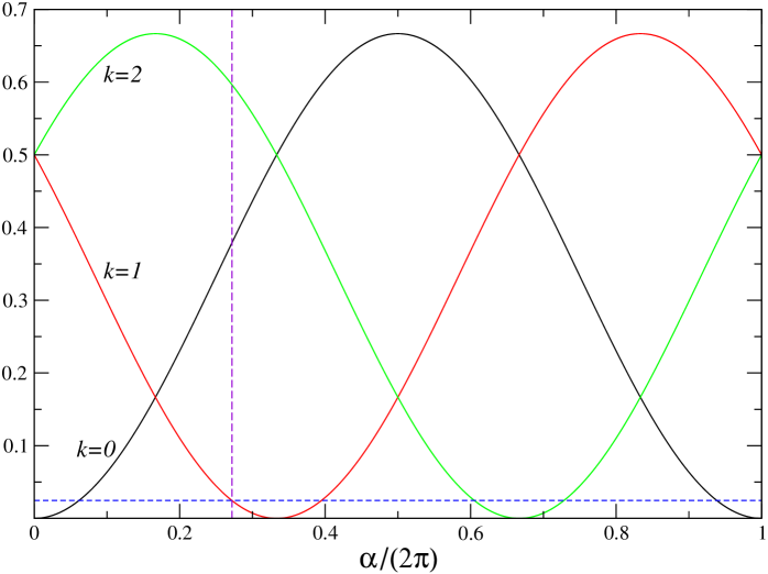
Figure 1: The functions $f_{k}(\alpha)$ of eq. (32). The dashed horizontal line indicates $s_{13}^{2}=0.0246$, the best-fit value of Forero et al. [2].

In that figure we also displayed a dashed horizontal line which indicates a phenomenologically realistic value of $s_{13}^{2}$. That horizontal line intersects each curve $f_{k}$ for two distinct values of $\alpha$. As an example, the vertical line in the figure shows the intersection point $\alpha=0.2718\left(2\pi\right)$ of $f_{1}$; in this example we have $s_{13}^{2}=f_{1}(\alpha)$, and then $c_{13}^{2}s_{23}^{2}$ would be either $f_{0}(\alpha)$ or $f_{2}(\alpha)$.

We can read off two facts from fig. 1. Firstly, for every value of $s_{13}^{2}$ there are two possible values of $s_{23}^{2}$. Secondly, all the intersection points lead to an identical relation between $s_{13}^{2}$ and $s_{23}^{2}$, i.e. the two values of $s_{23}^{2}$ are always the same no matter which $k$-curve one has chosen. Therefore, for simplicity we can take $k=0$ in eq. (32). Analytically, one then finds the relation

$$\left(1-s_{13}^{2}\right)^{2}\left(2s_{23}^{2}-1\right)^{2}=2s_{13}^{2}-3s_{13}^{4}.$$ (33)

Solving this equation for $s_{23}^{2}$ yields the two solutions

$$s_{23}^{2}=\frac{1}{2}\left(1\pm\frac{\sqrt{2s_{13}^{2}-3s_{13}^{4}}}{c_{13}^{2}}\right).$$ (34)

This is plotted in fig. 2.

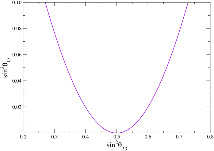
Figure 2: The relation between $s_{13}^{2}$ and $s_{23}^{2}$, a graphical rendering of eq. (34).

For definiteness in that figure we have allowed $s_{13}^{2}$ to vary between zero and $0.1$; in this limited range, the curve is almost a parabola [6].

Of course, in any definite model within our framework we must choose a well-defined value for $\alpha$, and thereby choose one point in the pseudo-parabola of fig. 2. We may, in particular, require that $\alpha$ is such that the model has a finite flavour symmetry group; a necessary condition for this is that $e^{i\alpha}$ should be a root of unity. In this case $\alpha/(2\pi)$ must be a rational number which approximates well one of the intersection points for the phenomenological value of $s_{13}^{2}$. In particular, the values of $\alpha$ in table 2 reproduce the phenomenological data quite well, as was first found in ref. [6].

$\alpha\left/\left(2\pi\right)\right.$	$s_{13}^{2}$	$s_{23}^{2}$
2/5, 3/5	0.028818	0.379101 or 0.620899
1/16, 15/16	0.025373	0.386653 or 0.613347
1/18, 5/18, 7/18, 11/18, 13/18, 17/18	0.020102	0.399242 or 0.600758

Table 2: Some rational values of $\alpha\left/\left(2\pi\right)\right.$ for which $s_{13}^{2}$, computed by using eq. (32), turns out to agree with the phenomenological data. The two corresponding values of $s_{23}^{2}$ follow from each value of $s_{13}^{2}$ according to eq. (34).

Furthermore, one may additionally require trimaximal mixing by using the additional, and independent, symmetry of eq. (27). Then the solar mixing angle is obtained from $s_{12}^{2}=1\left/\left(3c_{13}^{2}\right)\right.$. The requirement of TM₂ determines the $CP$-violating phase $\delta$ as [13]

$$\cos{\delta}=\frac{\left(1-2s_{13}^{2}\right)\left(1-2s_{23}^{2}\right)}{2s_{13}s_{23}c_{23}\sqrt{2-3s_{13}^{2}}}\,.$$ (35)

However, taking into account eq. (34), we simply find

$$\cos{\delta}=\mp 1,$$ (36)

where the upper (lower) sign corresponds to the upper (lower) sign in eq. (34). Thus, the $\mathbbm{Z}_{2}$ symmetry (28) together with TM₂ leads to $\delta=0$ or $\pi$, as was noticed for the viable cases of $U$ studied in ref. [6].

Since in the case discussed here we have determined two columns of $U$, the whole mixing matrix $U$ becomes, apart from possible permutations of the rows, determined as a function of $\alpha$:

$$U=\frac{1}{\sqrt{6}}\left(\begin{array}[]{ccccc}1+e^{i\alpha}&&\sqrt{2}&&1-e^{-i\alpha}\\ \omega^{2}+\omega e^{i\alpha}&&\sqrt{2}&&\omega-\omega^{2}e^{-i\alpha}\\ \omega+\omega^{2}e^{i\alpha}&&\sqrt{2}&&\omega^{2}-\omega e^{-i\alpha}\end{array}\right).$$ (37)

One may use this mixing matrix to check again that the $CP$-violating phase $\delta$ turns out to be trivial. However, the Majorana phases are non-trivial functions of $\alpha$, as can be read off from the following forms of the $k$-th entries in the first and third column:

$$U_{k1}=\sqrt{\frac{2}{3}}\cos\left(\frac{\alpha}{2}-\frac{2\pi k}{6}\right)e^{i\alpha/2}(-1)^{k},\quad U_{k3}=\sqrt{\frac{2}{3}}\sin\left(\frac{\alpha}{2}-\frac{2\pi k}{6}\right)i\,e^{-i\alpha/2}(-1)^{k}.$$ (38)

4 Conclusions

In this paper we have introduced a class of renormalizable models based on the double seesaw mechanism and on the soft breaking of flavour symmetries. In order to implement the double seesaw mechanism, the models possess three right-handed singlet fields $N_{jR}$, in addition to the $\nu_{jR}$ needed for the usual seesaw mechanism. Moreover, the models have an enlarged scalar sector compared to the Standard Model, namely four Higgs doublets and three complex scalar singlets. We stress that this is a rather minor field content in comparison to usual scenarios in model building with flavour symmetries, especially when those scenarios are supersymmetric.

Our class of models has both spontaneous and soft symmetry breaking. Spontaneous symmetry breaking occurs at two scales: at the scale $m_{X}$ through the VEVs of the scalar gauge singlets and at the Fermi scale through the VEVs of the Higgs doublets. Soft flavour symmetry breaking happens in the mass terms of the $N_{jR}$ at a scale $m_{\mathrm{soft}}$. If we assume that $m_{\mathrm{soft}}$ is much smaller than the Fermi scale, then the spontaneous symmetry breaking proceeds nearly unperturbed by the soft symmetry breaking. Due to the double seesaw mechanism, the mass scale $m_{\nu}$ of the light neutrinos is determined by

$$m_{\nu}\sim\frac{m_{Y}^{2}}{m_{X}^{2}}\,m_{\mathrm{soft}},$$ (39)

where $m_{Y}$ is at most of the order of the Fermi scale but might also be much smaller, since the masses of the charged leptons are considerably smaller than the Fermi scale. With $m_{\nu}\sim$ 0.1 eV, eq. (39) permits an estimate of $m_{\mathrm{soft}}/m_{X}^{2}$, but no independent determination of the soft-breaking scale and of the seesaw scale $m_{X}$.

Our flavour symmetries are arranged in such a way that, in an appropriate weak basis, the contribution to the lepton mixing matrix $U$ from the charged-lepton sector is given by $U_{\omega}$ of eq. (3), whereas the neutrino sector contributes a matrix $V$ constrained by either one or two $\mathbbm{Z}_{2}$ symmetries [5]. The matrix $V$ is exclusively determined by the Majorana mass matrix $M$ of the $N_{jR}$. Our class of models allows one to impose $\mathbbm{Z}_{2}$ symmetries which lead to virtually any of the forms of $U$ that have been proposed in the literature [5, 6]. This arbitrariness may be viewed as a weak point of our models, which on the other hand have the advantage of being renormalizable and natural in a technical sense.

We have explicitly discussed a model for TM₁. Then, by variation of the $\mathbbm{Z}_{2}$ symmetry of that model but keeping all its other flavour symmetries intact, we have shown that one can also achieve either TM₂ or a determination of the third column of $U$. The latter is enforced through a $\mathbbm{Z}_{2}$ symmetry depending on an angle $\alpha$. By varying $\alpha$, different values of $s_{13}^{2}$ are produced. In this way, we have explicitly reproduced the values of $s_{13}^{2}$ found in ref. [6].

Finally, combination of TM₂ and of the $\mathbbm{Z}_{2}$ symmetry depending on $\alpha$ results in the one-parameter mixing matrix of eq. (37), whose predictions we have discussed.

Appendix A The flavour symmetry group of the TM₁ model

We firstly recall the definition of the group series $\Delta(6n^{2})$, where $n$ is an integer. The easiest way to understand these groups is to conceive them as the subgroups of $SU(3)$ generated by

$$r=E,\quad s=-B,\quad t=T\equiv\mbox{diag}\left(1,\,\eta,\,\eta^{\ast}\right)\quad\mbox{with}\quad\eta\equiv\exp{\left(2\pi i/n\right)}.$$ (A1)

The definition of $\Delta(6n^{2})$ in ref. [15] uses a different set of generators $a$, $b$, $c$, and $d$ related to ours through $r=a$, $b=r^{-1}sr$, $c=rtr^{-1}$, and $d=t$.

Every group $\Delta(6n^{2})$ has $2(n-1)$ three-dimensional inequivalent irreducible representations (irreps) $\mathbf{3}^{(k\pm)}$ ($k=1,\ldots,n-1$), which are given in an appropriate basis by [15]

$$\mathbf{3}^{(k\pm)}:\quad r\to E,\quad s\to\mp B,\quad t\to\mbox{diag}\left(1,\,\eta^{k},\,\eta^{-k}\right).$$ (A2)

The flavour symmetry group of our TM₁ model is $G=G^{\prime}\times\mathbbm{Z}_{4}$. The group $G^{\prime}$ is the one generated by three transformations $g_{1,2,3}$. We know the following three representations of those transformations (in the first five columns of table 1):

$$D_{L},\ell_{R},\nu_{R}: g_{1}\to E,\ g_{2}\to A,\ g_{3}\to B,$$ (A3a)

$$N_{R}: g_{1}\to E,\ g_{2}\to A^{\ast},\ g_{3}\to D,$$ (A3b)

$$S: g_{1}\to E,\ g_{2}\to\mathbbm{1},\ g_{3}\to D.$$ (A3c)

The Higgs doublet $\phi_{0}$ is invariant under $G^{\prime}$. We leave the three Higgs doublets $\phi_{j}$ for later consideration.

Let us define a particular transformation $g\in G^{\prime}$ through $g\equiv g_{1}(g_{1}g_{3})^{2}g_{1}^{-1}$. One readily ascertains that

$$E\left(EB\right)^{2}E^{-1} = \mathbbm{1},$$ (A4a)

$$E\left(ED\right)^{2}E^{-1} = W\equiv{\rm diag}\left(1,-1,-1\right).$$ (A4b)

The unit matrix therefore represents $g$ in the representation of $D_{L}$, $\ell_{R}$, and $\nu_{R}$, while $W$ represents $g$ in the representation of $N_{R}$ and in the representation of $S$. Let us now define two further transformations $g^{\prime}_{2,3}\in G^{\prime}$ through $g^{\prime}_{2,3}\equiv g\,g_{2,3}$. Since

$$WD = B,$$ (A5a)

$$WA^{\ast} = {\rm diag}\left(1,\,e^{2\pi i/6},\,e^{-2\pi i/6}\right),$$ (A5b)

one concludes that the representations in eqs. (A3) might as well be given through

$$D_{L},\ell_{R},\nu_{R}: g_{1}\to E,\ g^{\prime}_{2}\to{\rm diag}\left(1,\,e^{2\pi i/3},\,e^{-2\pi i/3}\right),\ g^{\prime}_{3}\to B,$$ (A6a)

$$N_{R}: g_{1}\to E,\ g^{\prime}_{2}\to{\rm diag}\left(1,\,e^{2\pi i/6},\,e^{-2\pi i/6}\right),\ g^{\prime}_{3}\to B,$$ (A6b)

$$S: g_{1}\to E,\ g^{\prime}_{2}\to{\rm diag}\left(1,\,-1,\,-1\right),\ g^{\prime}_{3}\to B.$$ (A6c)

We conclude that $G^{\prime}=\Delta(216)$ with

$$D_{L},\ell_{R},\nu_{R}: {\mathbf{3}}^{(2-)},$$ (A7a)

$$N_{R}: {\mathbf{3}}^{(1-)},$$ (A7b)

$$S: {\mathbf{3}}^{(3-)}.$$ (A7c)

Actually, the argument for $\Delta(216)$, as developed above, boils down to the following. The symmetries $\mathbbm{Z}_{3}$ and $\mathbbm{Z}_{2}$ together generate a group $S_{4}$; this can be seen by considering the action of $\mathbbm{Z}_{3}$ and $\mathbbm{Z}_{2}$ on $N_{R}$ and on $S$. However, there is also $\mathbbm{Z}_{3}^{\prime}$. This suggests that

$$G^{\prime}\cong\left(\mathbbm{Z}_{3}^{\prime}\times\mathbbm{Z}_{3}^{\prime}\right)\rtimes S_{4}\cong\left(\mathbbm{Z}_{6}\times\mathbbm{Z}_{6}\right)\rtimes S_{3}\cong\Delta\left(6\times 6^{2}\right)=\Delta(216),$$ (A8)

where we have used $S_{4}\cong\left(\mathbbm{Z}_{2}\times\mathbbm{Z}_{2}\right)\rtimes S_{3}$ and $\mathbbm{Z}_{6}\cong\mathbbm{Z}_{3}^{\prime}\times\mathbbm{Z}_{2}$.

We lastly investigate the representation of $\phi$. This multiplet obviously transforms under $G^{\prime}$ as ${\bf 1}\oplus{\bf 2}$, where ${\bf 1}$ is invariant under $G^{\prime}$ and the two-dimensional irrep is given by

$${\bf 2}:\quad g_{1}\to\left(\begin{array}[]{cc}1&0\\ 0&1\end{array}\right),\quad g_{2}\to\left(\begin{array}[]{cc}\omega&0\\ 0&\omega^{2}\end{array}\right),\quad g_{3}\to\left(\begin{array}[]{cc}0&1\\ 1&0\end{array}\right).$$ (A9)

Therefore $g$ is represented in the ${\bf 2}$ by the $2\times 2$ unit matrix and

$${\bf 2}:\quad g_{1}\to\left(\begin{array}[]{cc}1&0\\ 0&1\end{array}\right),\quad g^{\prime}_{2}\to\left(\begin{array}[]{cc}\omega&0\\ 0&\omega^{2}\end{array}\right),\quad g^{\prime}_{3}\to\left(\begin{array}[]{cc}0&1\\ 1&0\end{array}\right).$$ (A10)

This is one of the four two-dimensional universal irreps of $\Delta(6n^{2})$ which exist whenever $n$ is a multiple of 3 [15, 16], as is the case for $\Delta(216)$.

Appendix B The $\phi_{j}$ potential

The symmetries $\mathbbm{Z}_{3}^{\prime}$ and $\mathbbm{Z}_{2}$ act on the Higgs doublets $\phi_{j}$ ($j=1,2,3$) as if they constituted a (reducible) triplet of a group $S_{3}$. Therefore, the potential for those three doublets alone is

$$V_{\phi} = \mu_{1}\,\phi_{1}^{\dagger}\phi_{1}+\mu_{2}\left(\phi_{2}^{\dagger}\phi_{2}+\phi_{3}^{\dagger}\phi_{3}\right)$$ (B1)

$$+\lambda_{1}\left(\phi_{1}^{\dagger}\phi_{1}\right)^{2}+\lambda_{2}\left[\left(\phi_{2}^{\dagger}\phi_{2}\right)^{2}+\left(\phi_{3}^{\dagger}\phi_{3}\right)^{2}\right]$$

$$+\lambda_{4}\,\phi_{1}^{\dagger}\phi_{1}\left(\phi_{2}^{\dagger}\phi_{2}+\phi_{3}^{\dagger}\phi_{3}\right)+\lambda_{5}\,\phi_{2}^{\dagger}\phi_{2}\,\phi_{3}^{\dagger}\phi_{3}$$

$$+\lambda_{4}^{\prime}\left(\phi_{1}^{\dagger}\phi_{2}\,\phi_{2}^{\dagger}\phi_{1}+\phi_{1}^{\dagger}\phi_{3}\,\phi_{3}^{\dagger}\phi_{1}\right)+\lambda_{5}^{\prime}\,\phi_{2}^{\dagger}\phi_{3}\,\phi_{3}^{\dagger}\phi_{2}$$

$$+\left[\lambda_{6}\,\phi_{1}^{\dagger}\phi_{2}\,\phi_{1}^{\dagger}\phi_{3}+\lambda_{7}\left(\phi_{1}^{\dagger}\phi_{2}\,\phi_{3}^{\dagger}\phi_{2}+\phi_{1}^{\dagger}\phi_{3}\,\phi_{2}^{\dagger}\phi_{3}\right)+{\rm H.c.}\right].$$

Let $\tilde{\lambda}_{4}\equiv\lambda_{4}+\lambda_{4}^{\prime}$ and $\tilde{\lambda}_{5}\equiv\lambda_{5}+\lambda_{5}^{\prime}$. Then, the VEV of the potential is

$$V_{0}\equiv\left\langle 0\left|V_{\phi}\right|0\right\rangle = \mu_{1}\left|v_{1}\right|^{2}+\mu_{2}\left(\left|v_{2}\right|^{2}+\left|v_{3}\right|^{2}\right)+\lambda_{1}\left|v_{1}\right|^{4}+\lambda_{2}\left(\left|v_{2}\right|^{4}+\left|v_{3}\right|^{4}\right)$$ (B2)

$$+\tilde{\lambda}_{4}\left|v_{1}\right|^{2}\left(\left|v_{2}\right|^{2}+\left|v_{3}\right|^{2}\right)+\tilde{\lambda}_{5}\left|v_{2}v_{3}\right|^{2}$$

$$+2\,\Re\left[\lambda_{6}{v_{1}^{\ast}}^{2}v_{2}v_{3}+\lambda_{7}v_{1}^{\ast}\left(v_{2}^{2}v_{3}^{\ast}+v_{3}^{2}v_{2}^{\ast}\right)\right].$$

It is hard to proceed analytically in the general case. We shall for the sake of simplification assume $\lambda_{6}=0$, even though there is no symmetry that supports that assumption. When $\lambda_{6}=0$ the two relative phases among $v_{1}$, $v_{2}$, and $v_{3}$ adjust so that $\lambda_{7}v_{1}^{\ast}v_{2}^{2}v_{3}^{\ast}$ and $\lambda_{7}v_{1}^{\ast}v_{3}^{2}v_{2}^{\ast}$ are both real and negative. One may then write

$$\tilde{V}_{0}=\tilde{\mu}_{2}\left(\left|v_{2}\right|^{2}+\left|v_{3}\right|^{2}\right)+\lambda_{2}\left(\left|v_{2}\right|^{4}+\left|v_{3}\right|^{4}\right)+\tilde{\lambda}_{5}\left|v_{2}v_{3}\right|^{2}-\left|\tilde{\lambda}_{7}\right|\left(\left|v_{2}^{2}v_{3}\right|+\left|v_{3}^{2}v_{2}\right|\right),$$ (B3)

where $\tilde{V}_{0}\equiv V_{0}-\mu_{1}\left|v_{1}\right|^{2}-\lambda_{1}\left|v_{1}\right|^{4}$, $\tilde{\mu}_{2}\equiv\mu_{2}+\lambda_{4}\left|v_{1}\right|^{2}$, and $\tilde{\lambda}_{7}\equiv 2\lambda_{7}v_{1}$. The equations for vacuum stability are

$$\frac{\partial\tilde{V}_{0}}{\partial\left|v_{2}\right|}=0 = 2\tilde{\mu}_{2}\left|v_{2}\right|+4\lambda_{2}\left|v_{2}\right|^{3}+2\tilde{\lambda}_{5}\left|v_{2}v_{3}^{2}\right|-2\left|\tilde{\lambda}_{7}v_{2}v_{3}\right|-\left|\tilde{\lambda}_{7}v_{3}^{2}\right|,$$ (B4a)

$$\frac{\partial\tilde{V}_{0}}{\partial\left|v_{3}\right|}=0 = 2\tilde{\mu}_{2}\left|v_{3}\right|+4\lambda_{2}\left|v_{3}\right|^{3}+2\tilde{\lambda}_{5}\left|v_{2}^{2}v_{3}\right|-2\left|\tilde{\lambda}_{7}v_{2}v_{3}\right|-\left|\tilde{\lambda}_{7}v_{2}^{2}\right|.$$ (B4b)

Subtracting the two eqs. (B4) from each other, we find that a solution with $\left|v_{2}\right|\neq\left|v_{3}\right|$ may exist provided

$$2\tilde{\mu}_{2} = -4\lambda_{2}\left(\left|v_{2}\right|^{2}+\left|v_{2}v_{3}\right|+\left|v_{3}\right|^{2}\right)+2\tilde{\lambda}_{5}\left|v_{2}v_{3}\right|-\left|\tilde{\lambda}_{7}\right|\left(\left|v_{2}\right|+\left|v_{3}\right|\right),$$ (B5a)

$$0 = \left(2\tilde{\lambda}_{5}-4\lambda_{2}\right)\left(\left|v_{2}^{2}v_{3}\right|+\left|v_{2}v_{3}^{2}\right|\right)-\left|\tilde{\lambda}_{7}\right|\left(\left|v_{2}\right|^{2}+\left|v_{3}\right|^{2}+3\left|v_{2}v_{3}\right|\right).$$ (B5b)

A solution to eqs. (B5) with $\left|v_{2}\right|$ and $\left|v_{3}\right|$ both positive should exist for appropriate values of the parameters. Notice the crucial role played by $\lambda_{7}$ in the existence of that solution—if $\lambda_{7}$ vanished then $\tilde{\lambda}_{5}$ would have to be equal to $2\lambda_{2}$ in order for eq. (B5b) to be satisfied; but $\tilde{\lambda}_{5}=2\lambda_{2}$ is not stable under renormalization because it is not supported by any extra symmetry of the potential.

The stability point of $\tilde{V}_{0}$ with $v_{2}\neq v_{3}$ will actually be a local minimum provided the matrix of the second derivatives of $\tilde{V}_{0}$ relative to $\left|v_{2}\right|$ and $\left|v_{3}\right|$, computed under the conditions of eqs. (B5), is positive definite. This means, apart from requiring positivity of the determinant of that matrix, we have to ensure that

$$4\lambda_{2}\left(2\left|v_{2}\right|^{2}-\left|v_{2}v_{3}\right|-\left|v_{3}\right|^{2}\right)+2\tilde{\lambda}_{5}\left(\left|v_{3}\right|^{2}+\left|v_{2}v_{3}\right|\right)-\left|\tilde{\lambda}_{7}\right|\left(\left|v_{2}\right|+3\left|v_{3}\right|\right) > 0,$$ (B6a)

$$4\lambda_{2}\left(2\left|v_{3}\right|^{2}-\left|v_{2}v_{3}\right|-\left|v_{2}\right|^{2}\right)+2\tilde{\lambda}_{5}\left(\left|v_{2}\right|^{2}+\left|v_{2}v_{3}\right|\right)-\left|\tilde{\lambda}_{7}\right|\left(\left|v_{3}\right|+3\left|v_{2}\right|\right) > 0.$$ (B6b)

We have moreover to ensure that this local minimum attains a lower value for $\tilde{V}_{0}$ than the solution to eqs. (B4) with $\left|v_{2}\right|=\left|v_{3}\right|$. In a more thorough study, we would also have to look for possible minima of $\tilde{V}_{0}$ which break the electric-charge invariance.

Appendix C The $S_{j}$ potential

The potential for the complex gauge singlets $S_{j}$ ($j=1,2,3$) must be invariant under the symmetries $\mathbbm{Z}_{3}$, $\mathbbm{Z}_{2}$, and $\mathbbm{Z}_{4}$, i.e. under $S_{1}\to S_{2}\to S_{3}\to S_{1}$, under $S_{2}\leftrightarrow-S_{3}$, and under $S_{j}\to iS_{j},\,\forall j$. Therefore,

$$V_{S} = \bar{\mu}\sum_{j=1}^{3}\left|S_{j}\right|^{2}+\bar{\lambda}_{1}\left(\sum_{j=1}^{3}\left|S_{j}\right|^{2}\right)^{2}+\bar{\lambda}_{2}\left(\left|S_{1}S_{2}\right|^{2}+\left|S_{1}S_{3}\right|^{2}+\left|S_{2}S_{3}\right|^{2}\right)$$ (C1)

$$+\left\{\bar{\lambda}_{3}\left(\sum_{j=1}^{3}S_{j}^{2}\right)^{2}+\bar{\lambda}_{4}\left[\left(S_{1}S_{2}\right)^{2}+\left(S_{1}S_{3}\right)^{2}+\left(S_{2}S_{3}\right)^{2}\right]{\rm+H.c.}\right\}$$

$$+\bar{\lambda}_{5}\left[\left(S_{1}^{\ast}S_{2}\right)^{2}+\left(S_{2}^{\ast}S_{3}\right)^{2}+\left(S_{3}^{\ast}S_{1}\right)^{2}+{\rm H.c.}\right],$$

with complex $\bar{\lambda}_{3}$ and $\bar{\lambda}_{4}$ but real $\bar{\lambda}_{5}$. The equations for vacuum stability are

$$0 = \bar{\mu}s_{1}^{\ast}+2\bar{\lambda}_{1}\left|s_{1}\right|^{2}s_{1}^{\ast}+\left(2\bar{\lambda}_{1}+\bar{\lambda}_{2}\right)\left(\left|s_{2}\right|^{2}+\left|s_{3}\right|^{2}\right)s_{1}^{\ast}$$ (C2a)

$$+4\bar{\lambda}_{3}s_{1}^{3}+\left(4\bar{\lambda}_{3}+2\bar{\lambda}_{4}\right)\left(s_{2}^{2}+s_{3}^{2}\right)s_{1}+2\bar{\lambda}_{5}\left({s_{2}^{\ast}}^{2}+{s_{3}^{\ast}}^{2}\right)s_{1},$$

$$0 = \bar{\mu}s_{2}^{\ast}+2\bar{\lambda}_{1}\left|s_{2}\right|^{2}s_{2}^{\ast}+\left(2\bar{\lambda}_{1}+\bar{\lambda}_{2}\right)\left(\left|s_{1}\right|^{2}+\left|s_{3}\right|^{2}\right)s_{2}^{\ast}$$ (C2b)

$$+4\bar{\lambda}_{3}s_{2}^{3}+\left(4\bar{\lambda}_{3}+2\bar{\lambda}_{4}\right)\left(s_{1}^{2}+s_{3}^{2}\right)s_{2}+2\bar{\lambda}_{5}\left({s_{1}^{\ast}}^{2}+{s_{3}^{\ast}}^{2}\right)s_{2},$$

$$0 = \bar{\mu}s_{3}^{\ast}+2\bar{\lambda}_{1}\left|s_{3}\right|^{2}s_{3}^{\ast}+\left(2\bar{\lambda}_{1}+\bar{\lambda}_{2}\right)\left(\left|s_{1}\right|^{2}+\left|s_{2}\right|^{2}\right)s_{3}^{\ast}$$ (C2c)

$$+4\bar{\lambda}_{3}s_{3}^{3}+\left(4\bar{\lambda}_{3}+2\bar{\lambda}_{4}\right)\left(s_{1}^{2}+s_{2}^{2}\right)s_{3}+2\bar{\lambda}_{5}\left({s_{1}^{\ast}}^{2}+{s_{2}^{\ast}}^{2}\right)s_{3}.$$

The potential $V_{S}$ has several accidental symmetries, like for instance under $S_{1}\to-S_{1}$ and under $S_{1}\leftrightarrow S_{2}$. Correspondingly, solutions to eqs. (C2) may exist with varying features, like $s_{1}=0$, $s_{1}=s_{2}\neq 0$, or $s_{1}=s_{2}=0$. In principle, a solution to eqs. (C2) with the three $s_{j}$ all nonzero and distinct may also exist.

In this paper we assume that the parameters of the potential are such that the solution to eqs. (C2) featuring $s_{1}=s_{2}=s_{3}\equiv s$, with

$$0=\bar{\mu}s^{\ast}+\left(6\bar{\lambda}_{1}+2\bar{\lambda}_{2}+4\bar{\lambda}_{5}\right)\left|s\right|^{2}s^{\ast}+\left(12\bar{\lambda}_{3}+4\bar{\lambda}_{4}\right)s^{3},$$ (C3)

is the actual global minimum of the potential. A proof that this can actually be achieved is beyond the scope of this paper.

Notice that $\bar{\mu}$ is supposed to be at the high (seesaw) scale $m_{X}$, and then the solution $s$ to eq. (C3) will be at that scale too—provided the coefficients $\bar{\lambda}_{k}$ ($k=1,\ldots,5$) are of order one.

Finding the minimum of the potential (C1) is a very difficult problem. However, in the special case where $\bar{\lambda}_{3}$ and $\bar{\lambda}_{4}$ are real and where $\bar{\lambda}_{2}$, $\bar{\lambda}_{3}$, $\bar{\lambda}_{4}$, and $\bar{\lambda}_{5}$ are all negative, one can actually prove that $s_{1}=s_{2}=s_{3}$ for an adequate range of the parameters of the potential. Indeed, in that case the minimum of $V_{S}$ with respect to the phases of the VEVs will be achieved when all three $s_{j}$ are real. One may then write

$$s_{1}=U\cos{\vartheta},\quad s_{2}=U\sin{\vartheta}\cos{\varphi},\quad s_{3}=U\sin{\vartheta}\sin{\varphi},$$ (C4)

with $U\geq 0$, $0\leq\vartheta\leq\pi$, and $0\leq\varphi\leq 2\pi$. Then,

$$V_{S}=\bar{\mu}U^{2}+\left(\bar{\lambda}_{1}+\bar{\lambda}_{3}\right)U^{4}+\left(\bar{\lambda}_{2}+\bar{\lambda}_{4}+2\bar{\lambda}_{5}\right)U^{4}\left(\cos^{2}{\vartheta}\sin^{2}{\vartheta}+\frac{\sin^{4}{\vartheta}\sin^{2}{2\varphi}}{4}\right).$$ (C5)

If $\bar{\lambda}_{2}+\bar{\lambda}_{4}+2\bar{\lambda}_{5}<0$, then the minimum will be attained for the values of $\vartheta$ and $\varphi$ that maximize $\cos^{2}{\vartheta}\sin^{2}{\vartheta}+\left.\left(\sin^{4}{\vartheta}\sin^{2}{2\varphi}\right)\right/\!4$. Assuming $s_{j}>0$ for $j=1,2,3$, these values are $\varphi=\pi/4$, $\vartheta=\arccos{1\left/\sqrt{3}\right.}$, corresponding to $s_{1}=s_{2}=s_{3}$.

The coefficients $\bar{\lambda}_{3}$ and $\bar{\lambda}_{4}$ could be real because of an additional $CP$ symmetry. That $CP$ symmetry would necessarily be broken at low scale through the VEVs $v_{j}$, which must have different phases so that the charged-lepton masses are non-degenerate.

In eq. (C1), the terms with coefficients $\bar{\lambda}_{3}$, $\bar{\lambda}_{4}$, and $\bar{\lambda}_{5}$ are sensitive to the phases of the VEVs $s_{j}$ and they prevent the emergence of any Goldstone bosons upon spontaneous symmetry breaking.

However, one can also take up the opposite stance and consider the case $\bar{\lambda}_{3}=\bar{\lambda}_{4}=0$, which is a special case of real coefficients $\bar{\lambda}_{3}$ and $\bar{\lambda}_{4}$. This may be enforced by a lepton-number ($L$) symmetry under which $D_{L}$, $\ell_{R}$, $\nu_{R}$, and $S$ all carry $L=1$. This lepton-number symmetry would be broken when the $S_{j}$ acquire VEVs and this breaking would lead to a Goldstone boson. However, that boson only couples to the right-handed neutrinos—through the term in eq. (11d)—and is, in practice, undetectable and harmless [18].

Acknowledgements:

The work of LL is supported through the Marie Curie Initial Training Network “UNILHC” PITN-GA-2009-237920 and also through the projects PEst-OE-FIS-UI0777-2013, PTDC/FIS-NUC/0548-2012, and CERN-FP-123580-2011 of the portuguese Fundação para a Ciência e a Tecnologia (FCT).

References

• [1] Y. Abe et al. (Double Chooz Coll.), Indication for the disappearance of reactor electron antineutrinos in the Double Chooz experiment, Phys. Rev. Lett. 108 (2012) 131801 [arXiv:1112.6353 [hep-ex]];
F.P. An et al. (Daya Bay Coll.), Observation of electron-antineutrino disappearance at Daya Bay, Phys. Rev. Lett. 108 (2012) 171803 [arXiv:1203.1669 [hep-ex]];
J.K. Ahn et al. (RENO Coll.), Observation of reactor electron antineutrino disappearance in the RENO experiment, Phys. Rev. Lett. 108 (2012) 191802 [arXiv:1204.0626 [hep-ex]].
• [2] D.V. Forero, M. Tórtola, and J.W.F. Valle, Global status of neutrino oscillation parameters after recent reactor measurements, Phys. Rev. D 86 (2012) 073012 [arXiv:1205.4018 [hep-ph]];
G.L. Fogli, E. Lisi, A. Marrone, D. Montanino, A. Palazzo, and A.M. Rotunno, Global analysis of neutrino masses, mixings and phases: Entering the era of leptonic $CP$ violation searches, Phys. Rev. D 86 (2012) 013012 [arXiv:1205.5254 [hep-ph]];
M.C. Gonzalez-Garcia, M. Maltoni, J. Salvado, and T. Schwetz, Global fit to three neutrino mixing: Critical look at present precision, J. High Energy Phys. 1212 (2012) 123 [arXiv:1209.3023 [hep-ph]].
• [3] P.F. Harrison, D.H. Perkins, and W.G. Scott, Tri-bimaximal mixing and the neutrino oscillation data, Phys. Lett. B 530 (2002) 167 [hep-ph/0202074].
• [4] C.H. Albright and W. Rodejohann, Comparing trimaximal mixing and its variants with deviations from tri-bimaximal mixing, Eur. Phys. J. C 62 (2009) 599 [arXiv:0812.0436 [hep-ph]];
C.H. Albright, A. Dueck, and W. Rodejohann, Possible alternatives to tri-bimaximal mixing, Eur. Phys. J. C 70 (2010) 1099 [arXiv:1004.2798 [hep-ph]].
• [5] C.S. Lam, Determining horizontal symmetry from neutrino mixing, Phys. Rev. Lett. 101 (2008) 121602 [arXiv:0804.2622 [hep-ph]];
C.S. Lam, The unique horizontal symmetry of leptons, Phys. Rev. D 78 (2008) 073015 [arXiv:0809.1185 [hep-ph]];
C.S. Lam, A bottom–up analysis of horizontal symmetry, arXiv:0907.2206 [hep-ph];
S.-F. Ge, D.A. Dicus, and W.W. Repko, $\mathbbm{Z}_{2}$ symmetry prediction for the leptonic Dirac $CP$ phase, Phys. Lett. B 702 (2011) 220 [arXiv:1104.0602 [hep-ph]];
H.-J. He and F.-R. Yin, Common origin of $\mu$ $\tau$ and $CP$ breaking in neutrino seesaw, baryon asymmetry, and hidden flavor symmetry, Phys. Rev. D 84 (2011) 033009 [arXiv:1104.2654 [hep-ph]];
R. de Adelhart Toorop, F. Feruglio, and C. Hagedorn, Discrete flavour symmetries in light of T2K, Phys. Lett. B 703 (2011) 447 [arXiv:1107.3486 [hep-ph]];
S.-F. Ge, D.A. Dicus, and W.W. Repko, Residual symmetries for neutrino mixing with a large $\theta_{13}$ and nearly maximal $\delta_{D}$, Phys. Rev. Lett.  108 (2012) 041801 [arXiv:1108.0964 [hep-ph]];
R. de Adelhart Toorop, F. Feruglio, and C. Hagedorn, Finite modular groups and lepton mixing, Nucl. Phys. B 858 (2012) 437 [arXiv:1112.1340 [hep-ph]];
H.-J. He and X.-J. Xu, Octahedral symmetry with geometrical breaking: New prediction for neutrino mixing angle $\theta_{13}$ and $CP$ violation, Phys. Rev. D 86 (2012) 111301 (R) [arXiv:1203.2908 [hep-ph]];
D. Hernandez and A.Yu. Smirnov, Lepton mixing and discrete symmetries, Phys. Rev. D 86 (2012) 053014 [arXiv:1204.0445 [hep-ph]];
C.S. Lam, Finite symmetry of leptonic mass matrices, Phys. Rev. D 87 (2013) 013001 [arXiv:1208.5527 [hep-ph]];
D. Hernandez and A.Yu. Smirnov, Discrete symmetries and model-independent patterns of lepton mixing, Phys. Rev. D 87 (2013) 053005 [arXiv:1212.2149 [hep-ph]];
B. Hu, Neutrino mixing and discrete symmetries, Phys. Rev. D 87 (2013) 033002 [arXiv:1212.2819 [hep-ph]].
• [6] M. Holthausen, K.S. Lim, and M. Lindner, Lepton mixing patterns from a scan of finite discrete groups, Phys. Lett. B 721 (2013) 61 [arXiv:1212.2411 [hep-ph]].
• [7] S. Antusch, S.F. King, C. Luhn, and M. Spinrath, Trimaximal mixing with predicted $\theta_{13}$ from a new type of constrained sequential dominance, Nucl. Phys. B 856 (2012) 328 [arXiv:1108.4278 [hep-ph]];
W. Rodejohann and H. Zhang, Simple two parameter description of lepton mixing, Phys. Rev. D 86 (2012) 093008 [arXiv:1207.1225 [hep-ph]];
E. Ma, Self-organizing neutrino mixing matrix, Phys. Rev. D 86 (2012) 117301 [arXiv:1209.3374 [hep-ph]];
C. Luhn, Trimaximal TM1 neutrino mixing in S4 with spontaneous $CP$ violation, Nucl. Phys. B 875 (2013) 80 [arXiv:1306.2358 [hep-ph]].
• [8] I. de Medeiros Varzielas and L. Lavoura, Flavour models for TM1 lepton mixing, J. Phys. G 40 (2013) 085002 [arXiv:1212.3247 [hep-ph]].
• [9] R.N. Mohapatra, Mechanism for understanding small neutrino mass in superstring theories, Phys. Rev. Lett.  56 (1986) 561;
R.N. Mohapatra and J.W.F. Valle, Neutrino mass and baryon number nonconservation in superstring models, Phys. Rev. D 34 (1986) 1642;
S.M. Barr, A different seesaw formula for neutrino masses, Phys. Rev. Lett. 92 (2004) 101601 [hep-ph/0309152];
T. Fukuyama, A. Ilakovac, T. Kikuchi, and K. Matsuda, Neutrino oscillations in a supersymmetric $SO(10)$ model with type-III see-saw mechanism, J. High Energy Phys. 0506 (2005) 016 [hep-ph/0503114];
P.S.B. Dev and A. Pilaftsis, Minimal radiative neutrino mass mechanism for inverse seesaw models, Phys. Rev. D 86 (2012) 113001 [arXiv:1209.4051 [hep-ph]].
• [10] P. Minkowski, $\mu\to e\gamma$ at a rate of one out of $10^{9}$ muon decays?, Phys. Lett. 67B (1977) 421;
T. Yanagida, Horizontal gauge symmetry and masses of neutrinos, in Proceedings of the workshop on unified theory and baryon number in the universe (Tsukuba, Japan, 1979), O. Sawata and A. Sugamoto eds., KEK report 79-18 (Tsukuba, Japan, 1979);
S.L. Glashow, The future of elementary particle physics, in Quarks and leptons, proceedings of the advanced study institute (Cargèse, Corsica, 1979), M. Lévy et al. eds. (Plenum Press, New York, U.S.A., 1980);
M. Gell-Mann, P. Ramond, and R. Slansky, Complex spinors and unified theories, in Supergravity, D.Z. Freedman and F. van Nieuwenhuizen eds. (North Holland, Amsterdam, The Netherlands, 1979);
R.N. Mohapatra and G. Senjanović, Neutrino mass and spontaneous parity violation, Phys. Rev. Lett. 44 (1980) 912.
• [11] W. Grimus and L. Lavoura, A model realizing the Harrison–Perkins–Scott lepton mixing matrix, J. High Energy Phys. 0601 (2006) 018 [hep-ph/0509239];
W. Grimus and L. Lavoura, Tri-bimaximal lepton mixing from symmetry only, J. High Energy Phys. 0904 (2009) 013 [arXiv:0811.4766 [hep-ph]].
• [12] W. Grimus, Discrete symmetries, roots of unity, and lepton mixing, J. Phys. G 40 (2013) 075008 [arXiv:1301.0495 [hep-ph]].
• [13] W. Grimus and L. Lavoura, A model for trimaximal lepton mixing, J. High Energy Phys. 0809 (2008) 106 [arXiv:0809.0226 [hep-ph]].
• [14] F. Feruglio, C. Hagedorn, and R. Ziegler, Lepton mixing parameters from discrete and $CP$ symmetries, J. High Energy Phys. 1307 (2013) 027 [arXiv:1211.5560 [hep-ph]];
G.-J. Ding, S.F. King, C. Luhn, and A.J. Stuart, Spontaneous $CP$ violation from vacuum alignment in $S_{4}$ models of leptons, J. High Energy Phys. 1305 (2013) 084 [arXiv:1303.6180 [hep-ph]].
F. Feruglio, C. Hagedorn, and R. Ziegler, $S_{4}$ and $CP$ in a SUSY model, arXiv:1303.7178 [hep-ph];
G.-J. Ding, S.F. King, and A.J. Stuart, Generalised $CP$ and $A_{4}$ family symmetry, J. High Energy Phys. 1312 (2013) 006 [arXiv:1307.4212 [hep-ph]].
• [15] A. Bovier, M. Lüling, and D. Wyler, Finite subgroups of $SU(3)$, J. Math. Phys.  22 (1981) 1543;
J.A. Escobar and C. Luhn, The flavor group $\Delta(6n^{2})$, J. Math. Phys.  50 (2009) 013524 [arXiv:0809.0639 [hep-th]].
• [16] W. Grimus and P.O. Ludl, Finite flavour groups of fermions, J. Phys. A 45 (2012) 233001 [arXiv:1110.6376 [hep-ph]].
• [17] P.M. Ferreira, W. Grimus, L. Lavoura, and P.O. Ludl, Maximal $CP$ violation in lepton mixing from a model with $\Delta(27)$ flavour symmetry, J. High Energy Phys. 1209 (2012) 128 [arXiv:1206.7072 [hep-ph]].
• [18] Y. Chikashige, R.N. Mohapatra, and R.D. Peccei, Are there real Goldstone bosons associated with broken lepton number?, Phys. Lett. 98B (1981) 265.