Analytical study of level crossings in the Stark-Zeeman spectrum of ground state OH

Abstract

The ground electronic, vibrational and rotational state of the OH molecule is currently of interest as it can be manipulated by electric and magnetic fields for experimental studies in ultracold chemistry and quantum degeneracy. Based on our recent exact solution of the corresponding effective Stark-Zeeman Hamiltonian, we present an analytical study of the crossings and avoided crossings in the spectrum. These features are relevant to non-adiabatic transitions, conical intersections and Berry phases. Specifically, for an avoided crossing employed in the evaporative cooling of OH, we compare our exact results to those derived earlier from perturbation theory.

1 Introduction

The OH molecule is currently the subject of wide theoretical as well as experimental investigation in the context of quantum computation Lev2006 , precision measurement Hudson2006 ; Kozlov2009 , ultracold collisions Avdeenkov2003 ; Ticknor2005 ; Sawyer2008 ; Tscherbul2010 and quantum degenerate fluids Quemener2012 . The ground state of the molecule displays both electric as well as magnetic dipole moments. This polar paramagnetic character of OH makes intermolecular interactions physically interesting Quemener2013 , and ensures that electric and magnetic fields can be extensively used to slow, guide, and trap ultracold OH molecules Bochinski2004 ; Meerakker2005 ; Sawyer2007 ; Stuhl2012 .

The effect of electric and magnetic fields on the OH molecule can be described by an eight dimensional effective Stark-Zeeman Hamiltonian when hyperfine structure, spin-orbit coupling and electric quadrupole effects are negligible, such as at strong fields or high molecular temperatures Stuhl2012 . This Hamiltonian has been successfully used to numerically model experimental data Quemener2012 ; Stuhl2012 . There have also been efforts towards obtaining analytical solutions to the Hamiltonian, as exemplified by the exact diagonalization of its field-dependent part Bohn2013 . Recently, our group presented the full analytical solutions for the $X^{2}\Pi_{3/2}$ OH ground state Hamiltonian in combined electric and magnetic fields, neglecting hyperfine structure. We also identified the underlying symmetry that enables the analytic solution Mishkat2013 .

The most prominent features visible in the corresponding molecular spectrum are multiple crossings and avoided crossings, which display rich behavior as the magnitudes and mutual orientation of the electric and magnetic fields vary (see Fig. 1), as has been shown in several experiments Quemener2012 ; Stuhl2012 . These (avoided) crossings are related to important physical phenomena such as Majorana transitions, responsible for OH trap loss Lara2008 ; Landau-Zener processes, which can be exploited for state transfer Stuhl2012 ; evaporative cooling, which is essential to Bose-Einstein condensation Quemener2012 ; and conical intersections, which provide pathways for molecular reactions Matsika2011 .

In the present work, we study analytically the crossings and avoided crossings in the spectrum of the OH ground state Stark-Zeeman Hamiltonian, using algebraic techniques established previously MishkatCrossingAJP ; MishkatCrossingPRA1 ; MishkatCrossingPRA2 . We show that although the (avoided) crossings display quite complex behavior, our analytical approach can organize and characterize this behavior systematically. Focusing on the experimentally relevant situation where the electric and magnetic field vectors are the tunable parameters Quemener2012 ; Stuhl2012 , we demonstrate that the locations of a particular subset of the (avoided) crossings can be found analytically. We use this knowledge to analyze in detail the gap at a specific avoided crossing important to the evaporative cooling of ground state OH molecules Quemener2012 and compare our exact results to those derived earlier using perturbation theory Stuhl2012 .

The remainder of this paper is organized as follows: In Section  2, we present the Stark-Zeeman Hamiltonian. We then discuss the crossings and avoided crossings in the spectrum in Section  3. Lastly, we conclude in Section  4.

2 Hamiltonian

The Hamiltonian of the $X^{2}\Pi_{3/2}$ OH molecule is given by Stuhl2012 ; Mishkat2013

$$H=H_{o}-\vec{\mu}_{e}\cdot\vec{E}-\vec{\mu}_{b}\cdot\vec{B},$$ (1)

where $H_{o}$ is the field-free Hamiltonian, $\vec{\mu}_{e}$ and $\vec{\mu}_{b}$ are the electric and magnetic molecular dipole moments, respectively, and $\vec{E}$ and $\vec{B}$ are the electric and magnetic fields, respectively. The matrix representation of this Hamiltonian has been obtained earlier in the literature as Stuhl2012

$$H_{M}=\left(\begin{array}[]{cc}A_{1}-A_{2}&-C\\ -C&A_{1}+A_{2}\\ \end{array}\right),$$ (2)

where

$$A_{1}=\frac{2}{5}\mu_{B}B \left(\begin{array}[]{cccc}-3&0&0&0\\ 0&-1&0&0\\ 0&0&1&0\\ 0&0&0&3\\ \end{array}\right),$$ (7)

$$A_{2}=\frac{\hbar\Delta}{2} \left(\begin{array}[]{cccc}1&0&0&0\\ 0&1&0&0\\ 0&0&1&0\\ 0&0&0&1\\ \end{array}\right),$$ (12)

$$C=\frac{\mu_{e}E}{5} \left(\begin{array}[]{cccc}-3\cos\theta&\sqrt{3}\sin\theta&0&0\\ \sqrt{3}\sin\theta&-\cos\theta&2\sin\theta&0\\ 0&2\sin\theta&\cos\theta&\sqrt{3}\sin\theta\\ 0&0&\sqrt{3}\sin\theta&3\cos\theta\\ \end{array}\right),$$ (17)

where $\Delta$ is the lambda-doubling parameter, $\mu_{B}$ is the Bohr magneton, $\mu_{e}$ is the magnitude of the molecular electric dipole moment, $E=|\vec{E}|$ and $B=|\vec{B}|$ are the electric and magnetic field magnitudes, respectively, and $\theta$ is the angle between the magnetic and electric field vectors. We note that this Hamiltonian has been used successfully to describe several experiments Quemener2012 ; Stuhl2012 . We also note that the validity of this Hamiltonian has two limitations: First, hyperfine as well as spin-orbit interactions have been neglected, which is justified for ongoing experiments Stuhl2012 . Second, the effect of the electric quadrupole term has been ignored. This term can become comparable to or larger than the magnetic dipole term (about 100 MHz at 100 Gauss) for a gradient in the electric field of a few percent.

The exact eigenvalues of $H_{M}$ can be found readily using Mathematica and have been provided in our earlier publication Mishkat2013 . In this article, the eigenvalues will be labeled as $\lambda_{i},i=1-8,$ as shown in Fig. 1 b) - f). We note that the analytical solutions maintain their energy ordering for a fixed nonzero electric field $E$ and angle $\theta$, and varying magnetic field strength.

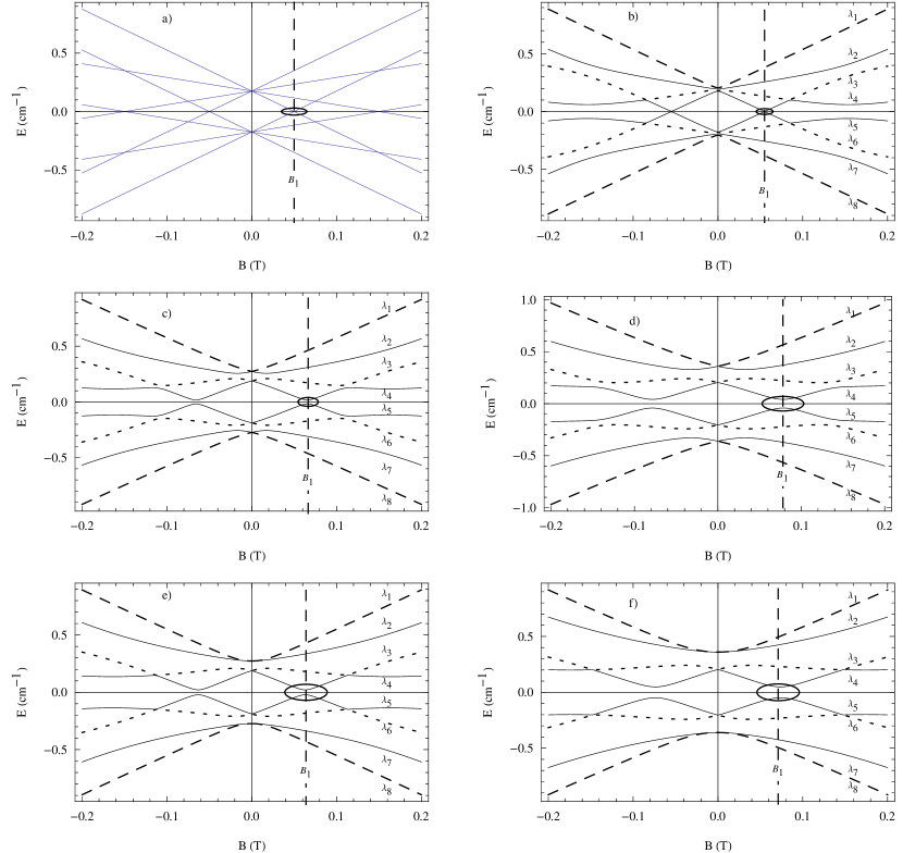
Figure 1: Spectrum of the Hamiltonian of Eq. (2) for $\Delta=2\pi\times 1.667$ GHz, $\mu_{e}=1.66$ D, and a) $\theta=\pi/3$, $E=0$ kV/cm, b) $\theta=\pi/3$, $E=1$ kV/cm, c) $\theta=\pi/3$, $E=2$ kV/cm, d) $\theta=\pi/3$, $E=3$ kV/cm, e) $\theta=\pi/2$, $E=2$ kV/cm, f) $\theta=\pi/2$, $E=3$ kV/cm. The horizontal axis represents the magnetic field in Tesla while the vertical axis represents energy in cm^-1. The analytic eigenvalues are labeled as $\lambda_{i},i=1-8$, consistent with the ordering in the text. The magnetic field location of the spectral feature of interest to this work, indicated by an ellipse, has been labeled as $B_{1}$. In a) $B_{1}$ indicates the position of a crossing which in b) - f) turns into an avoided crossing.

3 The discriminant

In principle, crossings in the spectrum, defined as the intersection between two eigenvalues, can be found by equating two eigenvalues $\lambda_{i}$ and $\lambda_{j}$ for $i\neq j$, $i,j=1...8$. Likewise and similarly, avoided crossings, defined as locations where the separation between two eigenvalues goes through a local minimum, can be found. Generally, this kind of approach is not very systematic, is tedious, and in view of the complexity of the eigenvalues and the multiplicity of tunable parameters in the present problem Mishkat2013 , not particularly insightful.

We will instead employ the more elegant and powerful algebraic approach, elaborated earlier in a series of articles MishkatCrossingAJP ; MishkatCrossingPRA1 ; MishkatCrossingPRA2 , which utilizes the discriminant of the characteristic polynomial of a matrix. The discriminant can always be obtained analytically, is available as a standard function in most symbolic computation software packages, and contains rather complete and accessible information about the crossings and avoided crossings in the spectrum as a function of the parameters of the Hamiltonian.

Since an extensive exposition of the algebraic technique we use in this article is already available in the literature, we will only summarize below the properties of the discriminant relevant to the present article.

1. The real roots of the discriminant correspond to the locations of crossings in the spectrum. Therefore, the simultaneous intersection of $n$ eigenvalues leads to ${n\choose 2}=n(n-1)/2$ crossings.

2. The real parts of complex roots of the discriminant correspond to the location of avoided crossings in the spectrum.

3. Every (avoided) crossing that occurs due to the tuning of a parameter $P$ of the Hamiltonian contributes a factor quadratic in $P$ to the discriminant.

The discriminant $D[H_{M}]$ of the matrix $H_{M}$ can be easily calculated either by using the eigenvalues $\lambda_{i}$ of $H_{M}$

$$\begin{array}[]{l}D[H_{M}]=\displaystyle\prod_{i<j}^{8}(\lambda_{i}-\lambda_{j})^{2},\\ \end{array}$$ (19)

or the characteristic polynomial of $H_{M}$

$$P(\lambda)=|H_{M}-\lambda I|=\displaystyle\sum_{n=0}^{8}p_{n}\lambda^{n},$$ (20)

whose coefficients $p_{n}$ have been published by us Mishkat2013 . The expressions for the discriminant are lengthy and complicated, and are thus shown only in Appendix A. Nonetheless, some exact conclusions can be drawn from them. We note, however, that analytic knowledge of the eigenvalues does not generally imply that the locations of all crossings and avoided crossings can be found exactly.

3.1 Factoring the discriminant

The discriminant $D[H_{M}]$ can be written as the product of three factors,

$$D[H_{M}]=f_{0}f_{1}f_{2}^{2},$$ (21)

whose explicit form has been provided in Appendix A. We will consider these factors to be polynomials in $B$, in order to find the avoided crossings as the magnetic field varies, following experiments Quemener2012 ; Stuhl2012 . We note that we could just as easily consider them to be polynomials in the electric field $E$ or the angle $\theta$ to find the avoided crossings as these two parameters are tuned.

The first factor of $D[H_{M}]$ is $f_{0}$, an eighth degree term in $B$. This term has eight real roots at $B=0$, corresponding to four real crossings at $B=0$ as seen in the spectrum, Fig. 1 b) - f). The second term, $f_{1},$ is an eighth-degree polynomial with only even order terms in $B$. It can thus be thought of as a quartic in $B^{2}$, making it analytically solvable. We will discuss this term in more detail in Appendix B. The third factor, $f_{2}^{2}$, is the square of a polynomial $f_{2}$ of degree 16, and also even in $B$. It does not seem to be generally solvable. We will discuss $f_{2}$ in Section  3.5.

The evenness (in $B$) can be traced to the presence of Kramer’s degeneracy due to the time-reversal symmetry of the system MishkatCrossingPRA2 . Reversing time implements the transformation

$$B\rightarrow-B,$$ (22)

which leaves the spectrum invariant as can be seen in Fig. 1. This symmetry causes the coefficients of the characteristic polynomial Eq. (20) to be even in $B$ and hence also all terms in the discriminant. A similar argument implies that the discriminant is also even in $E$. We note that in Appendix A we have used the variables $\tilde{B}=4\mu_{B}B,\tilde{E}=2\mu_{e}E$ and $\tilde{\Delta}=5\hbar\Delta$ to make the long expressions tidy. In the remainder of the article we will use either $E,B,\Delta$ or $\tilde{E},\tilde{B},\tilde{\Delta}$, as appropriate.

3.2 The magnetic field $B_{1}$

The roots of $f_{1}$ can be found by treating it as a quartic in $B^{2}$, which is analytically solvable Merriman1892 . From these solutions, we recover the eight roots of the original octic $f_{1}$ in the manner shown in Appendix B. In general, these roots, and therefore the magnetic field crossings and avoided crossings they correspond to, show rather complex behavior as a function of the parameters $E$ and $\theta$ as can be seen in Fig. 1. For instance, the positions of the (avoided) crossings depend on both parameters, and the angle determines whether or not a transition is avoided.

In this article, we will focus only on one particular situation which is of experimental interest Quemener2012 ; Stuhl2012 and concerns the circled crossing at $B_{1}$ in Fig. 1 a), where

$$B_{1}=\pm\frac{5\hbar\Delta}{12\mu_{B}},$$ (23)

which is a real root of $f_{1}$. In Fig. 1 a) this crossing is seen to occur for $E=0$ at the magnetic field of $\sim 0.05$T. In the presence of an electric field, this crossing turns into an avoided crossing between the eigenvalues $\lambda_{4}$ and $\lambda_{5}$, see Fig. 1 b) - f). The location $B_{1}$ of this avoided crossing has been derived in Appendix B and depends strongly on the electric field strength and the angle between the electric and magnetic field vectors. This dependence on the electric field strength was used experimentally to remove energetic molecules from an OH trap to implement evaporative cooling Quemener2012 . We note that this magnetic field location is also a function of $\Delta$, which is not tunable. In Fig. 2 and Fig. 3, respectively, we compare the variations of the exact analytical result for $B_{1}$ [Eq. (B)] with $E$ and $\theta$ to a simple approximation valid for low electric fields

$$\tilde{B}_{1}\simeq\frac{\tilde{\Delta}}{3}+\frac{3(3+\cos(2\theta))\tilde{E}^{2}}{8\tilde{\Delta}},$$ (24)

that we derive in Appendix B [Eq. (43)]. As can be seen from Fig. 2 and Fig. 3, this approximation is quite good for electric fields less than $500$V/cm.

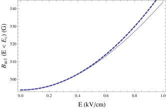
Figure 2: Magnetic field location $B_{1}$ versus electric field $E$ for $\theta=\pi/3$. The solid line is the exact result of Eq. (B), while the dotted line is the approximate expression of Eq. (43) for low electric fields.

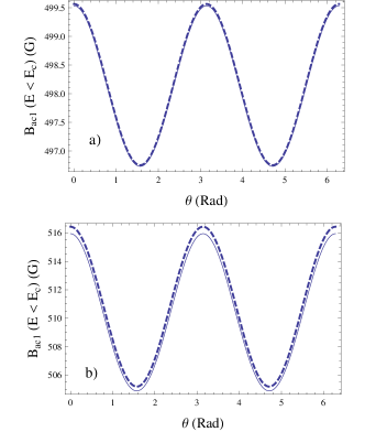
Figure 3: Magnetic field location $B_{1}$ versus $\theta$ for a) $E=250$V/cm and b) $E=500$V/cm. The solid line is the exact result of Eq. (B), while the dotted line is the approximate expression of Eq. (43) for low electric fields.

3.3 The $\delta_{-3/2}$ gap

The energy gap between $\lambda_{4}$ and $\lambda_{5}$ at $B_{1}$ was designated as $\delta_{-3/2}$ in an experimental study of Landau-Zener losses in an OH trap Stuhl2012 , see Fig. 1. Ground state OH molecules can be removed controllably from their confining trap through the $\delta_{-3/2}$ gap by tuning the direction and magnitude of an electric field. Thus, the scaling of the gap with $E$ and $\theta$ is of interest to current experiments Quemener2012 ; Stuhl2012 .

In the present article, we find the size of the gap analytically by inserting the value of the magnetic field $B_{1}$ into the eigenvalues $\lambda_{4}$ and $\lambda_{5}$,

$$\delta_{-3/2}=\lambda_{4}-\lambda_{5}=2\lambda_{4}(E,\theta,\Delta),$$ (25)

where we have used the fact that $\lambda_{5}=-\lambda_{4}$ to express the gap in terms of a single eigenvalue, $\lambda_{4}$. In the last step of Eq. (25), we have emphasized that $\delta_{-3/2}$ is only a function of $E,\theta$ and $\Delta$ since the magnetic field $B_{1}$ depends on those parameters.

In Fig. 4

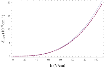
Figure 4: Energy gap $\delta_{-3/2}$ versus electric field $E$ for $\theta=\pi/3$. The solid line is the analytical result of Eq. (25), and the dotted line is a fit to $|aE^{3}|,$ (yielding $a=5830$) of the form in Eq. (26), as found earlier by perturbation theory Stuhl2012 .

and Fig. 5,

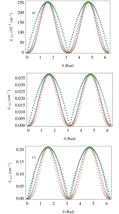
Figure 5: Energy gap $\delta_{-3/2}$ versus $\theta$ for a) $E=300$V/cm, b) $E=1.4$kV/cm and c) $E=4$kV/cm. In the plots, the solid line is the analytical result of Eq. (25), the solid dots correspond to a $|\sin\theta|$ curve, the crosses correspond to a $\sin^{2}\theta$ curve and the diamonds correspond to a $|\sin^{3}\theta|$ curve of the form in Eq. (26) as found earlier by perturbation theory Stuhl2012 . All curves are scaled to the amplitude of analytical result. In a) the $|\sin^{3}\theta|$ curve matches well the exact result, in b) the $\sin^{2}\theta$ is more appropriate, while in c) the $|\sin\theta|$ agrees best with the analytic answer.

we compare the field and angle scaling of our exact results to the result derived earlier using perturbation theory Stuhl2012 ,

$$\delta_{-3/2}\propto|E^{3}\sin^{3}\theta|.$$ (26)

From Fig. 4 we see that the perturbative scaling $\delta_{-3/2}\propto|E^{3}|$ is valid for electric fields less than about $70$V/cm for $\theta=\pi/3$. From Fig. 5 a), we infer that the perturbative scaling $\delta_{-3/2}\propto|\sin^{3}\theta|$ is accurate for low fields such as $300$V/cm. Our analytic results allow us to explore higher electric fields, at which the gap $\delta_{-3/2}$ shows rather different scaling behavior with respect to the angle $\theta$. In our calculations, for $E\geq 500$V/cm the variation of $\delta_{-3/2}$ with $|\sin\theta|$ deviates significantly from the cubic law of Eq. (26). For instance, from Fig. 5 b) we see that at $E=1.4$kV/cm, the behavior is much better described by a quadratic dependence, i.e. $\delta_{-3/2}\propto\sin^{2}\theta,$ while in Fig. 5 c) we see that at $E=4$kV/cm, the analytic curve follows closely the variation $\delta_{-3/2}\propto|\sin\theta|.$

3.4 The determinant

We note that $f_{1}$ can be written as

$$f_{1}=N_{a}(\lambda_{1}-\lambda_{8})^{2}(\lambda_{2}-\lambda_{7})^{2}(\lambda_{3}-\lambda_{6})^{2}(\lambda_{4}-\lambda_{5})^{2},$$ (27)

where $N_{a}=5^{8}$. This relation can be verified by using the analytical eigenvalue solutions $\lambda_{i}$ Mishkat2013 . Equation (27) implies that the zeros of $f_{1}$ correspond to (avoided) crossings only between opposite energy pairs $\lambda_{i}$ and $\lambda_{9-i}$ in the spectrum. In general, these are the only (avoided) crossings whose locations can be obtained analytically. Further, by using the relation Mishkat2013

$$\lambda_{i}=-\lambda_{9-i},\,\,\,i=1,\ldots 8$$ (28)

together with Eq. (27), we find that

$$f_{1}=N_{b}\prod\limits_{j=1}^{8}\lambda_{j}=N_{b}|H_{M}|,$$ (29)

where $N_{b}=10^{8}.$ Thus, $f_{1}$ is proportional to the determinant $|H_{M}|$ of the matrix $H_{M}$. Therefore, at every crossing implied by the real roots of $f_{1},|H_{M}|$ vanishes, which implies that at least two of the eigenvalues have zero energy. As a check, in the case of the $\delta_{-3/2}$ gap considered above, it can be verified that at $E=0$ the two eigenvalues which cross, and which have zero energy, are $\lambda_{4}$ and $\lambda_{5}$, see Fig. 1 a).

3.5 The roots of $f_{2}$

The last factor in the discriminant $D[H_{M}]$ is $f_{2}^{2}.$ All (avoided) crossings accounted for by $f_{2}$ occur between levels which are not opposite energy pairs. The polynomial is of order 16 in $B$. However, since it is even in $B$, it can be thought of as an octic in $B^{2}$. This octic does not seem to be solvable in general. This implies that the magnetic field locations such as for the avoided crossing gaps labeled $\delta_{\pm 1/2}$ in earlier work Stuhl2012 cannot be found analytically. A detailed analysis of the solvability of $f_{2}$ requires using the condition that the corresponding Galois group is solvable BasuBook . However, in view of the complexity of the coefficients, the result is not likely to be very illuminating, and we have not pursued this avenue.

The polynomial $f_{2}$ does yield analytic roots for some special cases. The simplest case, a trivial one, occurs when $E=0.$ In that case,

$$f_{2}=512\tilde{B}^{8}\tilde{\Delta}^{4}\left(4\tilde{B}^{4}-5\tilde{B}^{2}\tilde{\Delta}^{2}+\tilde{\Delta}^{4}\right)^{2},$$

corresponding to crossings at

$$B_{c}=0,\pm\frac{5\hbar\Delta}{8\mu_{B}},\pm\frac{5\hbar\Delta}{4\mu_{B}}.$$

Less trivial, and possibly experimentally relevant solvable configurations occur when the electric and magnetic fields are (anti)parallel [$\theta=(\pi)0$] or perpendicular $(\theta=\pi/2)$. In these cases, $f_{2}$ reduces to

$$f_{2}[\theta=0] =512\left(\tilde{\Delta}^{4}+10\tilde{\Delta}^{2}\tilde{E}^{2}+9\tilde{E}^{4}\right)\left(4\tilde{B}^{8}+4\tilde{E}^{8}\right.$$

$$\left.-5\tilde{B}^{6}\left(\tilde{\Delta}^{2}+5\tilde{E}^{2}\right)-5\tilde{B}^{2}\tilde{E}^{4}\left(\tilde{\Delta}^{2}+5\tilde{E}^{2}\right)\right.$$

$$\left.+\tilde{B}^{4}\left(\tilde{\Delta}^{4}+10\tilde{\Delta}^{2}\tilde{E}^{2}+42\tilde{E}^{4}\right)\right)^{2},$$

$$f_{2}\left[\theta=\frac{\pi}{2}\right] =512\tilde{B}^{4}\tilde{\Delta}^{4}\left(-4\tilde{B}^{2}+\tilde{\Delta}^{2}+8\tilde{E}^{2}\right)^{2}\left(\tilde{B}^{8}+\tilde{E}^{8}\right.$$

$$\left.-2\tilde{B}^{6}\left(\tilde{\Delta}^{2}-2\tilde{E}^{2}\right)+\tilde{B}^{2}\tilde{E}^{4}\left(\tilde{\Delta}^{2}+4\tilde{E}^{2}\right)\right.$$

$$\left.+\tilde{B}^{4}\left(\tilde{\Delta}^{4}+8\tilde{\Delta}^{2}\tilde{E}^{2}+6\tilde{E}^{4}\right)\right),$$

$$f_{2}\left[\theta=\pi\right] =512\left(\tilde{\Delta}^{4}+10\tilde{\Delta}^{2}\tilde{E}^{2}+9\tilde{E}^{4}\right)\left(4\tilde{B}^{8}+4\tilde{E}^{8}\right.$$

$$\left.-5\tilde{B}^{6}\left(\tilde{\Delta}^{2}+5\tilde{E}^{2}\right)-5\tilde{B}^{2}\tilde{E}^{4}\left(\tilde{\Delta}^{2}+5\tilde{E}^{2}\right)\right.$$

$$\left.+\tilde{B}^{4}\left(\tilde{\Delta}^{4}+10\tilde{\Delta}^{2}\tilde{E}^{2}+42\tilde{E}^{4}\right)\right)^{2},$$ (30)

for $\theta=0,\pi/2,$ and $\pi$, respectively, and the locations of all the crossings and avoided crossings in the spectrum of $H_{M}$ can be found analytically in a straightforward way.

4 Conclusion

We have presented an analytical level-crossing study of the $X^{2}\Pi_{3/2}$ state of the OH molecule, which is relevant to ongoing experiments. We have clarified the set of crossings and avoided crossings whose locations can be found analytically. We have analyzed a particular avoided crossing which is important to nonadiabatic transitions leading to evaporative cooling of OH molecules towards Bose-Einstein condensation. We have derived exact as well as approximate analytic expressions for the magnetic field location of this avoided crossing. We have also found an analytic expression for the gap at the avoided crossing, and compared its scaling properties with respect to electric field and angle, with results derived earlier from perturbation theory.

Appendix A Discriminant

The three factors in Eq. (21) are

$$f_{0} =\left(\frac{\sqrt{3}}{156250(2^{1/4})}\right)^{8}\tilde{B}^{8},$$

$$f_{1} =81\tilde{B}^{8}-36\left[9\cos(2\theta)\tilde{E}^{2}+5\tilde{\Delta}^{2}\right]\tilde{B}^{6}+2\left[59\tilde{\Delta}^{4}\right.$$

$$\left.+81\left(2+\cos(4\theta)\right)\tilde{E}^{4}+54\left(7-2\cos(2\theta)\right)\tilde{\Delta}^{2}\tilde{E}^{2}\right]\tilde{B}^{4}$$

$$-4\left(\tilde{\Delta}^{2}+9\tilde{E}^{2}\right)\left[5\tilde{\Delta}^{4}+\left(9\tilde{E}^{2}-7\tilde{\Delta}^{2}\right)\tilde{E}^{2}\cos(2\theta)\right.$$

$$\left.+21\tilde{\Delta}^{2}\tilde{E}^{2}\right]\tilde{B}^{2}+\left(\tilde{\Delta}^{4}+9\tilde{E}^{4}+10\tilde{\Delta}^{2}\tilde{E}^{2}\right)^{2},$$

$$f_{2} =g_{16}\tilde{B}^{16}+g_{14}\tilde{B}^{14}+g_{12}\tilde{B}^{12}+g_{10}\tilde{B}^{10}+g_{8}\tilde{B}^{8}$$

$$+g_{6}\tilde{B}^{6}+g_{4}\tilde{B}^{4}+g_{2}\tilde{B}^{2}+g_{0},$$

where $\tilde{\Delta}=5\hbar\Delta,\tilde{B}=4\mu_{B}B$ and $\tilde{E}=2\mu_{e}E$ and

$$g_{16} =8192\left[\Delta^{4}+5\left(1+\cos(2\theta)\right)\Delta^{2}\tilde{E}^{2}+72\cos^{4}\theta\tilde{E}^{4}\right],$$

$$g_{14} =-2048\left[\right.9\cos^{4}\theta\left(9+41\cos(2\theta)\right)\tilde{E}^{6}+10\tilde{\Delta}^{6}$$

$$\left.+\cos^{2}\theta\left(247+343\cos(2\theta)\right)\tilde{\Delta}^{2}\tilde{E}^{4}+150\cos^{2}\theta\tilde{\Delta}^{4}\tilde{E}^{2}\right],$$

$$g_{12} =64\left[\right.264\tilde{\Delta}^{8}+240\left(15+7\cos(2\theta)\right)\tilde{\Delta}^{6}\tilde{E}^{2}$$

$$\left.+2\left(7613+9308\cos(2\theta)+1311\cos(4\theta)\right)\tilde{\Delta}^{4}\tilde{E}^{4}\right.$$

$$\left.+9\cos^{4}\theta\left(3155+2052\cos(2\theta)+2481\cos(4\theta)\right)\tilde{E}^{8}\right.$$

$$\left.+4\cos^{2}\theta\left(8599+13060\cos(2\theta)+3501\cos(4\theta)\right)\tilde{\Delta}^{2}\tilde{E}^{6}\right],$$

$$g_{10} =-32\left[160\tilde{\Delta}^{10}+16\left(203+47\cos(2\theta)\right)\tilde{\Delta}^{8}\tilde{E}^{2}+4\left(5685\right.\right.$$

$$\left.\left.+3884\cos(2\theta)+631\cos(4\theta)\right)\tilde{\Delta}^{6}\tilde{E}^{4}+36\cos^{4}\theta\left(1620\right.\right.$$

$$\left.\left.+5367\cos(2\theta)+1188\cos(4\theta)+1025\cos(6\theta)\right)\tilde{E}^{10}\right.$$

$$\left.+4\cos^{2}\theta\left(39498+56409\cos(2\theta)+27750\cos(4\theta)\right.\right.$$

$$\left.\left.+2903\cos(6\theta)\right)\tilde{\Delta}^{2}\tilde{E}^{8}+\left(72962+100955\cos(2\theta)\right.\right.$$

$$\left.\left.+33550\cos(4\theta)+4533\cos(6\theta)\right)\tilde{\Delta}^{4}\tilde{E}^{6}\right],$$

$$g_{8} =8\left[64\tilde{\Delta}^{12}+192\tilde{\Delta}^{10}\tilde{E}^{2}\left(9+\cos(2\theta)\right)\right.$$

$$\left.+8\tilde{\Delta}^{8}\tilde{E}^{4}\left(2193+1012\cos(2\theta)+339\cos(4\theta)\right)\right.$$

$$\left.+16\tilde{\Delta}^{6}\tilde{E}^{6}\left(5651+6444\cos(2\theta)+3093\cos(4\theta)\right.\right.$$

$$\left.\left.+252\cos(6\theta)\right)+72\tilde{E}^{12}\cos^{4}\theta\left(8253+6804\cos(2\theta)\right.\right.$$

$$\left.\left.+7786\cos(4\theta)+900\cos(6\theta)+625\cos(8\theta)\right)\right.$$

$$\left.+4\tilde{\Delta}^{2}\tilde{E}^{10}\cos^{2}\theta\left(199593+305817\cos(2\theta)\right.\right.$$

$$\left.\left.+135562\cos(4\theta)+38183\cos(6\theta)+1165\cos(8\theta)\right)\right.$$

$$\left.+\tilde{\Delta}^{4}\tilde{E}^{8}\left(305959+533164\cos(2\theta)+289236\cos(4\theta)\right.\right.$$

$$\left.\left.+55892\cos(6\theta)+3077\cos(8\theta)\right)\right],$$

$$g_{6} =\left[-\tilde{\Delta}^{10}\left(64+2816\cos(2\theta)+2240\cos(4\theta)\right)\right.$$

$$\left.-16\tilde{\Delta}^{8}\tilde{E}^{2}\left(354+4215\cos(2\theta)+3326\cos(4\theta)\right.\right.$$

$$\left.\left.+105\cos(6\theta)\right)-1152\tilde{E}^{10}\cos^{4}\theta\left(1620+5367\cos(2\theta)\right.\right.$$

$$\left.\left.+1188\cos(4\theta)+1025\cos(6\theta)\right)-64\tilde{\Delta}^{2}\tilde{E}^{8}\cos^{2}\theta\left(67824\right.\right.$$

$$\left.\left.+129141\cos(2\theta)+44446\cos(4\theta)+12779\cos(6\theta)\right.\right.$$

$$\left.\left.-1070\cos(8\theta)\right)-4\tilde{\Delta}^{6}\tilde{E}^{4}\left(38821+159112\cos(2\theta)\right.\right.$$

$$\left.\left.+117620\cos(4\theta)+11768\cos(6\theta)-921cos(8\theta)\right)\right.$$

$$\left.+\tilde{\Delta}^{4}\tilde{E}^{6}\left(-1413318-3053506\cos(2\theta)-1941176\cos(4\theta)\right.\right.$$

$$\left.\left.-392525\cos(6\theta)+11646\cos(8\theta)+4879\cos(10\theta)\right)\right]\tilde{E}^{4},$$

$$g_{4} =4\left[1575\tilde{\Delta}^{8}+\tilde{\Delta}^{8}\left(1616\cos(2\theta)+844\cos(4\theta)\right)\right.$$

$$\left.+144\tilde{E}^{8}\cos^{4}\theta\left(3155+2052\cos(2\theta)+2481\cos(4\theta)\right)\right.$$

$$\left.+8\tilde{\Delta}^{2}\tilde{E}^{6}\cos^{2}\theta\left(91042+69141\cos(2\theta)+52350\cos(4\theta)\right.\right.$$

$$\left.\left.-11253\cos(6\theta)\right)+432\tilde{\Delta}^{8}\cos(6\theta)+\tilde{\Delta}^{4}\tilde{E}^{4}\left(198181\right.\right.$$

$$\left.\left.+249080\cos(2\theta)+118740\cos(4\theta)+38536\cos(6\theta)\right.\right.$$

$$\left.\left.-21113\cos(8\theta)\right)+2\tilde{\Delta}^{6}\tilde{E}^{2}\left(15185+1675\cos(2\theta)\right.\right.$$

$$\left.\left.+8580\cos(4\theta)+3856\cos(6\theta)-2133\cos(8\theta)\right)\right.$$

$$\left.-243\tilde{\Delta}^{8}\cos(8\theta)\right]\tilde{E}^{8},$$

$$g_{2} =512\cos^{2}\theta\left[\tilde{\Delta}^{6}\left(3-64\cos(2\theta)\right)-36\tilde{E}^{6}\cos^{2}\theta\left(9\right.\right.$$

$$\left.\left.+41\cos(2\theta)\right)+21\tilde{\Delta}^{6}\cos(4\theta)+2\tilde{\Delta}^{4}\tilde{E}^{2}\left(-3\right.\right.$$

$$\left.\left.-436\cos(2\theta)+139\cos(4\theta)\right)+4\tilde{\Delta}^{2}\tilde{E}^{4}\left(-118\right.\right.$$

$$\left.\left.-655\cos(2\theta)+183\cos(4\theta)\right)\right]\tilde{E}^{12},$$

$$g_{0} =4096\tilde{E}^{16}\left(\tilde{\Delta}^{2}+9\tilde{E}^{2}\right)\cos^{2}\theta\left(5\tilde{\Delta}^{2}+\tilde{E}^{2}\right.$$

$$\left.+\left(-3\tilde{\Delta}^{2}+\tilde{E}^{2}\right)\cos(2\theta)\right).$$

Appendix B Roots of $f_{1}$

The roots of $f_{1}$ can be found using standard methods. Hence we supply only an outline of the derivation below. To find the roots of $f_{1}$ it is convenient to divide by the coefficient of the first term to obtain a new polynomial

$$F_{1}=\frac{f_{1}}{81}=\tilde{B}^{8}+c_{6}\tilde{B}^{6}+c_{4}\tilde{B}^{4}+c_{2}\tilde{B}^{2}+c_{0},$$ (31)

where

$$c_{6} =-\frac{20}{9}\tilde{\Delta}^{2}-4\tilde{E}^{2}\cos 2\theta,$$

$$c_{4} =\frac{118}{81}\tilde{\Delta}^{4}+\frac{4}{3}\left(7-2\cos(2\theta)\right)\tilde{E}^{2}\tilde{\Delta}^{2}+2\tilde{E}^{4}\left(2+\cos(4\theta)\right),$$

$$c_{2} =-\frac{4\left(\tilde{\Delta}^{2}+9\tilde{E}^{2}\right)}{81}\left(5\tilde{\Delta}^{4}+9\cos(2\theta)\tilde{E}^{4}\right.$$

$$\left.-7\left(\cos(2\theta)-3\right)\tilde{\Delta}^{2}\tilde{E}^{2}\right),$$

$$c_{0} =\frac{\left(\tilde{\Delta}^{4}+9\tilde{E}^{4}+10\tilde{\Delta}^{2}\tilde{E}^{2}\right)^{2}}{81}.$$

The solutions to Eq. (32) are succinctly analyzed in terms of the corresponding depressed quartic StegunBook ; WikiQuartic

$$f(u)=u^{4}+qu^{2}+ru+s,$$ (32)

where

$$u = \tilde{B}^{2}+\frac{c_{6}}{4},$$

$$q = c_{4}-\frac{3c_{6}^{2}}{8},$$

$$r = \frac{1}{8}(8c_{2}-4c_{4}c_{6}+c_{6}^{3}),$$

$$s = c_{0}-\frac{1}{256}c_{6}(64c_{2}-16c_{4}c_{6}+3c_{6}^{3}).$$ (33)

Since we are looking for complex roots of $F_{1},$ which correspond to avoided crossings, we assume a root for Eq. (32) of the form $u=x+iy$, where $x$ and $y$ are both real. With this assumption, the depressed quartic returns a root with real $x$ and $y$ only if the discriminant of the resolvent cubic WikiQuartic $\Delta_{c}$ obeys the relation

$$\Delta_{c}<0,$$ (34)

where

$$\Delta_{c}=-\left(\frac{2}{3}\right)^{2}\left(\frac{32}{3}\right)^{9}\left(\tilde{\Delta}\tilde{E}^{2}\right)^{4}\left(\tilde{\Delta}^{2}+9\tilde{E}^{2}\right)^{3}\sin^{8}\theta G_{c},$$ (35)

with

$$G_{c} = 32\tilde{\Delta}^{6}+16\tilde{E}^{2}\tilde{\Delta}^{4}(25-23\cos(2\theta))$$

$$+576\tilde{E}^{4}\tilde{\Delta}^{2}\sin^{2}\theta(7-\cos(2\theta))$$

$$+2592\tilde{E}^{6}\sin^{2}\theta\cos^{4}\theta.$$

From Eq. (35) it follows that $\Delta_{c}<0$ if $G_{c}>0,$ which in turn is readily apparent from Eq. (B) as $G_{c}$ is the sum of four terms which are all positive.

In this case, the complex roots of the depressed [Eq. (32)], as well as the original [Eq. (31)] quartic can be found analytically. It turns out that as the electric field $\tilde{E}$ is tuned, the real parts of the two pairs of complex conjugate roots of Eq. (32) become degenerate at

$$C_{r}=0,$$ (37)

where

$$C_{r}=\frac{2^{1/3}}{24D_{B}}\left(2q^{2}+24s\right)+\frac{2^{2/3}}{24}D_{B}-\frac{q}{6},$$

$$D_{B}=3^{1/3}\left(2/3q^{3}+9r^{2}-24qs\right.$$

$$\left.+\sqrt{12q^{3}r^{2}+81r^{4}-48q\left(q^{3}+9r^{2}\right)s+384q^{2}s^{2}-768s^{3}}\right)^{1/3}.$$

This occurs at the (angle-dependent) critical field

$$\tilde{E}_{c}=\frac{\tilde{\Delta}}{\sqrt{1-2\cos\left(2\theta\right)}}.$$ (39)

Physically, this corresponds (for $\tilde{B}>0$) to the coincidence of two avoided crossings between the eigenvalues $\lambda_{4}$ and $\lambda_{5}$. Since we are interested always in the avoided crossing $\delta_{-3/2}$ occurring at the lower magnetic field, we find the real and imaginary parts of the roots of Eq. (32) in terms of the squared variable $\tilde{B}_{1}^{\prime 2}$ for $\tilde{E}<\tilde{E}_{c}$ to be

$$\Re[\tilde{B}^{\prime 2}_{1}]=-\sqrt{C_{r}}-\frac{c_{6}}{4},\,\,\,\Im[\tilde{B}^{\prime 2}_{1}]=\sqrt{-\frac{r}{4\sqrt{C_{r}}}+C_{r}+\frac{q}{2}}.\\$$ (40)

Above the critical electric field ($\tilde{E}>\tilde{E}_{c})$ the corresponding expressions are instead

$$\Re[\tilde{B}^{\prime 2}_{1}]=\sqrt{C_{r}}-\frac{c_{6}}{4},\,\,\,\,\Im[\tilde{B}^{\prime 2}_{1}]=\sqrt{\frac{r}{4\sqrt{C_{r}}}+C_{r}+\frac{q}{2}}.\\$$ (41)

Note the difference in sign for the $\sqrt{C_{r}}$ terms between Eqs. (40) and (41).

Finally, the magnetic field location $\tilde{B}_{1}$ of the avoided crossing $\delta_{-3/2}$ below the critical field $\tilde{E}_{c}$ is readily found MostowskiBook , i.e.

$$\tilde{B}_{1} =\sqrt{\frac{\Re[\tilde{B}^{\prime 2}_{1}]+\sqrt{\Re[\tilde{B}^{\prime 2}_{1}]^{2}+\Im[\tilde{B}^{\prime 2}_{1}]^{2}}}{2}}.$$

An approximate expression correct to lowest order in the electric field $\tilde{E}$ is found to be

$$\tilde{B}_{1}(\tilde{E}<\tilde{E}_{c})\simeq\frac{\tilde{\Delta}}{3}+\frac{3(3+\cos(2\theta))\tilde{E}^{2}}{8\tilde{\Delta}}.$$ (43)

In the text, Fig. 2 and Fig. 3 compare the approximation of Eq. (43) to the exact result of Eq. (B), showing the initial quadratic dependence with the electric field and the $\cos 2\theta$ angular dependence. An expression for the magnetic field loation of the avoided crossing above the critical electric field can also be found similarly.

References

- (1) B. L. Lev, E. R. Meyer, E. R. Hudson, B. C. Sawyer, J. L. Bohn and J. Ye , Phys. Rev. A 74, 061402(R) (2006).
- (2) E. R. Hudson, H. J. Lewandowski, B. C. Sawyer and J. Ye, Phys. Rev. Lett. 96, 143004 (2006).
- (3) M. G. Kozlov, Phys. Rev. A 80, 022118 (2009).
- (4) A. V. Avdeenkov and J. L. Bohn, Phys. Rev. Lett. 90, 043006 (2003).
- (5) C. Ticknor and J. L. Bohn, Phys. Rev. A 71, 022709 (2005).
- (6) B. C. Sawyer, B. K. Stuhl, D. Wang, M. Yeo and J. Ye, Phys. Rev. Lett. 101, 203203 (2008).
- (7) T. V. Tscherbul, Z. Pavlovic, H. R. Sadeghpour, R. Cote, and A. Dalgarno, Phys. Rev. A 82, 022704 (2010).
- (8) B. K. Stuhl, M. T. Hummon, M. Yeo, G. Quemener, J. L. Bohn and J. Ye, Nature 492, 396 (2012).
- (9) G. Quemener and J. L. Bohn, Phys. Rev. A 88, 012706 (2013).
- (10) J. R. Bochinski. E. R. Hudson, H. J. Lewandowski, and J. Ye, Phys. Rev. A 70, 043410 (2004).
- (11) S. Y. T. van de Meerakker, P. H. M. Smeets, N. Vanhaecke, R. T. Jongma, and G. Meijer, Phys. Rev. Lett. 94, 023004 (2005).
- (12) B. C. Sawyer, B. L. Lev, E. R. Hudson, B. K. Stuhl, M. Lara, J. L. Bohn, and J. Ye, Phys. Rev. Lett. 98, 253002 (2007).
- (13) B. K. Stuhl, M. Yeo, B. C. Sawyer, M. T. Hummon and J. Ye, Phys. Rev. A 85, 033427 (2012).
- (14) M. Garttner, J. J. Olmiste, P. Schmelcher, and R. Gonzalez-Ferez, arxiv:1301.4586v1 (2013).
- (15) J. L. Bohn and G. Quemener, arxiv:1301.2590v1 (2013).
- (16) M. Bhattacharya, Z. Howard and M. Kleinert, Phys. Rev. A 88, 012503 (2013).
- (17) M. Lara, B. L. Lev and J. L. Bohn, Phys. Rev. A 78, 033433 (2008).
- (18) S. Matsika and P. Krause, Ann. Rev. of Phys. Chem. 62, 621(2011).
- (19) M. Bhattacharya, Am. J. Phys. 75, 942 (2007).
- (20) M. Bhattacharya and C. Raman, Phys. Rev. A, 75, 033405 (2007).
- (21) M. Bhattacharya and C. Raman, Phys. Rev. A 75, 033406 (2007).
- (22) M. Merriman, Bull. New York Math. Soc., 1, 202 (1892).
- (23) M. Abramowitz, M. and I. A. Stegun (Eds.), Handbook of Mathematical Functions with Formulas, Graphs, and Mathematical Tables. New York: Dover.
- (24) E. W. Weisstein, ”Quartic Equation.” From MathWorld–A Wolfram Web Resource, http://mathworld.wolfram.com/QuarticEquation.html
- (25) A. Mostowski and M. Stark, Introduction to Higher Algebra, Pergamom Press, New York, 1964.
- (26) S. Basu, R. Pollack and M. F. Roy, Algorithms in Real Algebraic Geometry, Springer-Verlag, Berlin, 2003.