Feedback-induced nonlinearity and superconducting on-chip quantum optics

Abstract

Quantum coherent feedback has been proven to be an efficient way to tune the dynamics of quantum optical systems and, recently, those of solid-state quantum circuits. Here, inspired by the recent progress of quantum feedback experiments, especially those in mesoscopic circuits, we prove that superconducting circuit QED systems, shunted with a coherent feedback loop, can change the dynamics of a superconducting transmission line resonator, i.e., a linear quantum cavity, and lead to strong on-chip nonlinear optical phenomena. We find that bistability can occur under the semiclassical approximation, and photon anti-bunching can be shown in the quantum regime. Our study presents new perspectives for engineering nonlinear quantum dynamics on a chip.

I Introduction

Feedback, which is the core of modern control theory Astrom , has been applied to the control of quantum dynamical systems Wiseman ; Dong ; Altafini ; Kerckhoff0 for over twenty years, after Belavkin’s pioneering work on quantum filtering and control Belavkin . Now, it has been extensively studied for various problems in quantum system, such as optical squeezing Wiseman2 ; JGough1 ; Iida0 , spin squeezing LKThomsen , quantum state stabilization JWang ; Stockton ; Handel ; Ibarcq , quantum error correction and noise suppression DVitali ; Ganesan ; Jzhang ; Fzhang ; Qi ; Vijay ; CAhn_and_ACDoherty ; Xue , entanglement control JWang_and_Wiseman ; Yamamoto ; zLiu , cooling AHopkins_and_KJacobs ; jzhangl ; Greenberg ; Woolley , and rapid quantum measurement JohnComes ; jzhangl2 .

There are mainly two different quantum feedback control methods: the measurement-based feedback Wisman1 ; Mabuchi ; Doherty ; Mancini and coherent feedback Wisman4 ; Lloyd ; Yanagisawa ; James ; Gough . In a typical measurement-based feedback-control optical system, a probe field usually transmits through the quantum system to be controlled and then the information is extracted. Afterwards, the extracted information is fed into a classical controller which generates the desired control signal. This control signal is then fed back to tune the dynamics of the controlled system. The simplest measurement-based feedback control protocol is the so-called direct Markovian feedback Wisman1 , in which the measurement output is directly feedback to steer the dynamics of the controlled system. Both the time-delay in the feedback loop and the filtering effects induced by the integral components are omitted, which leads to the so-called Markovian approximation. However, due to the inevitable time delay and filtering effects in the feedback loop, such a simplification may not be valid in various cases. To solve this problem, another measurement-based feedback protocol, called “Bayesian feedback”, was proposed Doherty , in which the measurement output signal is fed into a classical state estimator, e.g., a series of integral components, to estimate the state of the controlled quantum system and then fed into a classical controller to obtain a state-based feedback control. It is worth noting that both direct Markovian feedback and Bayes feedback have been experimentally demonstrated in optical cavity systems Riste ; Sciarrino ; Brakhane ; Yonezawa ; Gieseler ; Berry0 ; Kubanek ; Sayrin ; Zhou and solid-state circuits Vijay .

Although great progress has been achieved for measurement-based feedback, there are still many problems left to be solved. The main open problems of the measurement-based feedback approaches include: (1) the time scale of the general quantum dynamics is too fast to be manipulated in real time by currently-available classical controllers; and (2), more essentially, the back-action brought by the quantum measurement keeps dumping entropy into the system before the feedback attempts to reduce it. One possible way to solve this is to avoid the introduction of the measurement step and use a fully quantum feedback loop to control the quantum system, which leads to a new feedback mechanism called coherent feedback. The simplest way to introduce coherent feedback is to couple directly the controlled quantum system with the quantum controller Lloyd , which is called “direct coherent feedback”. An alternative approach is the field-mediated coherent feedback Yanagisawa ; James ; Gough , in which the controlled quantum system and the quantum controller are connected by an intermediate quantum field. The direction of the information flow in the feedback loop is naturally determined by the propagation direction of the quantum field, and thus it is easier to be realized in experiments Nelson ; Mabuchi1 ; Zhou0 ; Kerckhoff ; Iida .

The existing studies about coherent feedback were mainly focused on linear quantum systems. This is because previous studies on coherent feedback are mainly focused on quantum optical systems Jaksch , where the nonlinear effects are too weak to be observed. However, recent progress shows that nonlinear quantum optical phenomena induced by the strong interaction between photons and solid-state components can be observed Birnbaum ; Fink ; Bishop in solid-state systems, such as quantum dots, superconducting circuits, and silicon-based waveguides Politi ; Matthews ; Berry . In our previous study J.Zhang , we found that, different from measurement-based feedback, quantum coherent feedback can induce and amplify the quantum nonlinear effects, and then modulate the dynamics of the controlled system. We call this “quantum feedback nonlinearization”. However, in this study, the quantum nonlinear effects are induced by the nonlinear dissipative coupling between the controlled quantum system and the intermediate quantum field. The quantum feedback loop is just linear.

In this paper, we propose a different nonlinear coherent feedback control strategy and apply it to superconducting circuits. The main difference between this strategy and our previous study in Ref. J.Zhang is that here a nonlinear component, i.e., a nonlinear superconducting device You ; Hoffman ; Nation ; Tornes ; Buluta0 ; Georgescu ; Buluta1 ; Nation1 ; Youf0 ; Youf1 ; Xiang0 , is embedded in the feedback loop, and the coupling between the controlled systems and the intermediate quantum field is linear. Such a design is easier to be realized in experiments Kerckhoff .

This paper is organized as follows. In Sec. II, we summarize results from the quantum input-output theory and the theory of coherent feedback-control networks, which will be used here afterwards. In Sec. III, we present our design of nonlinear coherent feedback systems in supercoducting quantum circuits, and then analyze the dynamics of the controlled systems in the semiclassical regime (strong-driving regime) to show bistability in Sec. IV, and the quantum regime (weak-driving regime) to show quantum nonlinear optical phenomena, such as photon antibunching effects in Sec. V. Conclusions and discussions are given in Sec. VI.

II PRELIMINARIES

The basic model for a quantum input-output system can be presented by a controlled system driven by an external bath, where the bath consists of different modes which can be described by a continuum of harmonic oscillators. We assume that $\hbar=1$ in the following discussions. The Hamiltonian for such a system can be expressed as

$$H= H_{\rm sys}+H_{B}+H_{\rm int}$$ (1)

$$H_{B}= \int_{-\infty}^{+\infty}\omega b^{{\dagger}}(\omega)b(\omega){\rm d}\omega$$

$$H_{\rm int}= i\int_{-\infty}^{+\infty}\left[\kappa(\omega)b^{{\dagger}}(\omega)a-{\rm h.c.}\right]{\rm d}\omega$$

where $a$ is the annihilation operator of the system; and $b^{{\dagger}}(\omega)$, $b(\omega)$ are the creation and annihilation operators of the bath mode with frequency $\omega$ satisfying

$$\left[b(\omega),b^{{\dagger}}(\tilde{\omega})\right]=\delta\left(\omega-\tilde{\omega}\right).$$ (2)

The commutator $\left[\cdot,\cdot\right]$ is defined as $\left[A,B\right]=AB-BA$. $H_{\rm sys}$ is the free Hamiltonian of the system, which interacts with the bath modes with coupling operator $a$ and coupling strengths $\kappa(\omega)$. In the interaction picture, Equation (1) can be rewritten as

$$H_{\rm eff}=H_{\rm sys}+i\int_{-\infty}^{+\infty}\left[\kappa(\omega)b^{{\dagger}}(\omega)e^{i\omega t}a-{\rm h.c.}\right]{\rm d}\omega.$$ (3)

Under the Markov approximation, i.e., the coupling strength is constant for all frequencies $\kappa(\omega)=\sqrt{\gamma/2\pi}$, the Hamiltonian $H_{\rm eff}$ can be expressed as

$$H_{\rm eff}=H_{\rm sys}+i\left[b^{\dagger}_{\rm in}L-L^{\dagger}b_{\rm in}\right].$$ (4)

$L=\sqrt{\gamma}a$ is the Lindblad operator induced by the coupling between the system and the quantum field. Also,

$$b_{\rm in}(t)=\frac{1}{\sqrt{2\pi}}\int_{-\infty}^{+\infty}b(\omega)e^{-i\omega t}{\rm d}\omega$$ (5)

is defined as the input quantum field Jacobs .

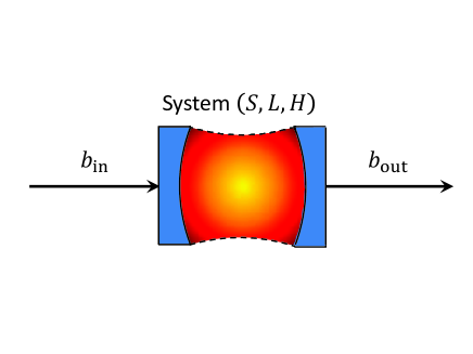
Figure 1: (Color online) Schematic diagram of the quantum input-output system with the input field $b_{\rm in}$ and the output field $b_{\rm out}$. Here, $S$, $L$, $H$ are, respectively, the scattering matrices, the Lindblad operator, and the Hamiltonian of the input-output system.

Let us consider a general input-output model as in Fig. 1. The input field $b_{\rm in}=[b_{1}(t),{\cdots},b_{n}(t)]^{T}$, where the superscript denotes transposition, satisfies the commutation relations $[b_{i}(t),b^{{\dagger}}_{j}(s)]={\delta}_{ij}(t-s)$, and transmits through a beam-splitter described by an $n{\times}n$ unitary scattering matrix $S$, such that $S^{{\dagger}}S=SS^{{\dagger}}=I$. The input field interacts with the controlled system with the Hamiltonian $H$ which leads to the dissipation channel represented by the Lindblad operator $L=[L_{1},{\cdots},L_{n}]^{T}$. The unitary evolution operator $U(t)$ of the total system composed of the controlled system and the input field can be described by the following quantum stochastic differential equation J.Zhang :

$$\frac{{\rm d}{U(t)}}{{\rm d}t}= b^{{\dagger}}_{\rm in}(t)(S-I)U(t)b_{\rm in}(t)+b^{{\dagger}}_{\rm in}(t)LU(t)$$ (6)

$$-L^{{\dagger}}SU(t)b_{\rm in}(t)-\left[\frac{1}{2}L^{{\dagger}}L-iH\right]U(t),$$

with initial condition $U(0)=I$, where $I$ is the identity operator. The output field is defined by

$$b_{\rm out}(t)=U^{{\dagger}}(t)SU(t)b_{\rm in}(t)+U^{{\dagger}}(t)LU(t).$$ (7)

It can be seen that the above quantum input-output system can be fully determined by a set of operators $(S,L,H)$. For a quantum Markovian cascaded system as shown in Fig. 2(a), in which the output field of the first component $(S_{1},L_{1},H_{1})$ acts as the input field of the second system $(S_{2},L_{2},H_{2})$, the dynamics of the total system can be described by

$$\left({S^{\prime}},{L^{\prime}},{H^{\prime}}\right),$$ (8)

with

$${S^{\prime}}\equiv S_{2}S_{1},\ {L^{\prime}}\equiv L_{2}+S_{2}L_{1},$$

$${H^{\prime}}\equiv H_{1}+H_{2}+\frac{i}{2}\left(L_{1}^{{\dagger}}S_{2}^{{\dagger}}L_{2}-L_{2}^{{\dagger}}S_{2}L_{1}\right).$$

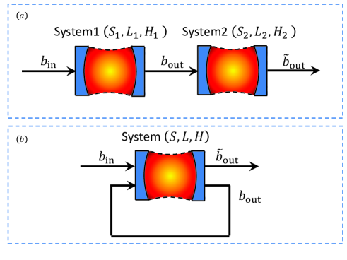
Figure 2: (Color online) Schematic diagram of the cascade system with two cascaded-connected components in (a) and the feedback-control systems in (b), which can be seen as the controlled system cascaded-connected with itself.

In particular, we feed the output of the system $(S,L,H)$ back and take it as the input of the same system to construct a direct coherent-feedback network, as in Fig. 2(b). From Eq. (8), such a feedback network can be described by J.Zhang :

$$\left(\tilde{S},\tilde{L},\tilde{H}\right),$$ (9)

with

$$\tilde{{S}}\equiv S^{2},\ \tilde{{L}}\equiv L+SL,$$

$$\tilde{{H}}\equiv H+\frac{i}{2}L^{{\dagger}}(S^{{\dagger}}-S)L.$$

III Nonlinear coherent feedback in superconducting circuits

In Fig. 3 we present our proposed nonlinear coherent feedback system using superconducting circuits. The controlled system is a one-dimensional transmission line resonator (TLR) with distributed inductor $L_{s}$ and capacitance $C_{s}$, which has two input channels and two output channels. The TLR is driven by the input field $b_{\rm in}$ through the dissipation channel represented by the Lindblad operator $L=\sqrt{\gamma}a$. Also $a$ is the annihilation operator of the quantum field in the TLR, and $\gamma$ is the corresponding dissipation rate. The output field of the TLR is then fed into a controller composed of another TLR coupled to a dc-SQUID-based superconducting charge qubit, which is driven by either a current or voltage source G. Wendin ; Beltran . The quantum controller interacts with the intermediate field via the dissipation channel with Lindblad operator $L_{c}$. Afterwards, the output of the quantum controller is fed back to act as the input field $\tilde{b}_{\rm in}$ of the controlled system via the dissipation channel $L_{f}$ to close the coherent feedback loop.

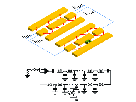
Figure 3: (Color online) Schematic diagram of the coherent feedback network using superconducting quantum circuits. The controlled system is a TLR which can be considered as a linear cavity. The controller in the feedback loop is another TLR coupled with a dc-SQUID-based superconducting charge qubit which acts as a nonlinear component.

If we assume the inductance of the SQUID to be small, we can neglect the magnetic energy of the circulating currents. Under the two-level approximation, the Hamiltonian of the controller can be expressed as Liu1

$$H_{qT} =\frac{1}{2}\omega_{0}\sigma_{z}+\omega_{c}c^{{\dagger}}c+g\left(c\sigma_{+}+c^{{\dagger}}\sigma_{-}\right)$$ (10)

$$+\Omega\left(\sigma_{+}e^{-i\omega_{1}t}+\sigma_{-}e^{i\omega_{1}t}\right)+\varepsilon\left(c^{{\dagger}}e^{-i\omega_{2}t}+ce^{i\omega_{2}t}\right),$$

where $c$ is the annihilation operator of the quantized electromagnetic field in the TLR coupled to the dc-SQUID based superconducting charge qubit; $\Omega$ is the Rabi frequency describing the interaction between the qubit and the classical field; $g$ is the coupling strength between the qubit and the quantized electromagnetic field; and $\varepsilon$ is the strength of the driving field applied to the cavity mode. If the Rabi frequency $\Omega$ is large enough, such that $\Omega\gg g^{2}/\Delta_{qT}$, and in the large-detuning regime,

$$\Delta_{qT}=\omega_{c}-\omega_{0}\gg g,$$

we can write an effective Hamiltonian which can be reexpressed as Liu1 (see derivations in Appendix A)

$$H_{\rm eff}=\omega_{c}c^{{\dagger}}c+\Omega\sigma_{z}+\frac{g^{4}}{2\Omega\Delta_{qT}^{2}}\left(c^{{\dagger}}c\right)^{2}\sigma_{z}$$ (11)

If the qubit is adiabatically placed in its ground state $|-\rangle$, the effective Hamiltonian in Eq. (11) can be expressed as

$$H_{qT}^{\prime} =\omega_{c}c^{{\dagger}}c-\chi\left(c^{{\dagger}}c\right)^{2}$$ (12)

$$+\varepsilon\left(c^{{\dagger}}e^{-i\omega_{2}t}+ce^{i\omega_{2}t}\right),$$

where $\chi={g^{4}}/\left({2\Omega\Delta_{qT}^{2}}\right)$. In the $(S,L,H)$ notation, the quantized electromagnetic field can be represented by:

$$(1,\sqrt{\kappa}{c},H_{qT}^{\prime}),$$ (13)

where $\kappa$ is the decay rate of the quantized electromagnetic field. The controlled linear cavity (TLR) can be described as $(1,\sqrt{\gamma}{a},\omega_{s}{a^{{\dagger}}a})$, where $\gamma$ and $a$ are the decay rate and the annihilation operator of the cavity, respectively.

The total coherent feedback system can be considered as a cascade system of the subsystem $(1,\sqrt{\gamma}{a},\omega_{s}{a^{{\dagger}}a})$, the quantum controller $(1,\sqrt{\kappa}{c},H_{qT}^{\prime})$, and the subsystem $(1,\sqrt{\gamma_{f}}{a},\omega_{s}{a^{{\dagger}}a})$, which can be written as

$$(S^{\prime\prime},L^{\prime\prime},H^{\prime\prime}),$$ (14)

with

$$S^{\prime\prime}=1,\ L^{\prime\prime}=\sqrt{\kappa}{c}+(\sqrt{\gamma}+\sqrt{\gamma_{f}}){a},$$

$$H^{\prime\prime}=\omega_{s}{a^{{\dagger}}a}+H_{qT}^{\prime}+\frac{i}{2}(\sqrt{\kappa\gamma}-\sqrt{\kappa\gamma_{f}})(a^{{\dagger}}c-c^{{\dagger}}a).$$

In the rotating reference frame with unitary transformation $V(t)=\exp\left[i\left(\omega_{2}{c^{{\dagger}}}c+\omega_{2}{a^{{\dagger}}}a\right)t\right]$, the total Hamiltonian can be represented as

$${H}_{\rm tot}= \Delta_{s}{a^{{\dagger}}}a+{\Delta}c^{{\dagger}}c-\chi\left(c^{{\dagger}}\right)^{2}c^{2}-\varepsilon(c^{{\dagger}}+c)$$ (15)

$$+\frac{i}{2}(\sqrt{\kappa\gamma}-\sqrt{\kappa\gamma_{f}})(a^{{\dagger}}c-c^{{\dagger}}a),$$

where

$$\Delta_{s}=\omega_{s}-\omega_{2},\ \Delta=\omega_{c}-\omega_{2},$$

are the detuning frequencies.

With the decrease of the strength of the external driving field, different optical phenomena can be observed. In the strong-driving semi-classical regime, semiclassical nonlinear bistability effects can be found, while in the weak-driving quantum regime, quantum nonlinear phenomena such as anti-bunching can be observed.

IV Nonlinear on-chip optics by coherent feedback: semi-classical regime

We first consider the case when the external field imposed on the controller is strong, where we can observe semiclassical nonlinear phenomena such as optical bistability. Optical bistability is a typical nonlinear phenomenon which has been observed in various systems Gibbs ; Rempe ; Sauer ; Gupta ; Brennecke ; Xiao . It has also been demonstrated that quantum feedback can modulate such kinds of nonlinear effects. For example, the recent experiment Kerckhoff showed that two coupled superconducting tunable Kerr cavities (TKCs) connected in a feedback configuration can demonstrate semiclassical on-chip nonlinear optical phenomena. The reflected phase from the TKC is a nonlinear function of the driving amplitude and thus the TKC acts as a typical nonlinear component, which means that both the controlled system and the controller are nonlinear systems. In contrast to this design, in our system, as shown in Fig. 3, the controlled system is a linear system and the controller is nonlinear. We now want to show how the nonlinear controller modulates the controlled linear dynamics, making the controlled system nonlinear.

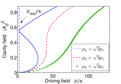
Figure 4: (Color online) Magnitude of the steady field $|A_{0}|^{2}$ in the controlled cavity versus the intensity of the driving field $|\varepsilon|$, with system parameters: $\Delta_{s}/{2\pi}=100$ MHz, $\Delta/{2\pi}=4.9$ MHz, $\chi/{2\pi}=10$ MHz, $\gamma/{2\pi}=6$ MHz, $\gamma_{f}/{2\pi}=8$ MHz and $\kappa/2\pi=3$ MHz. In the parameter regime $p_{2}>\sqrt{3}p_{1}$, we observe a hysteresis curve, indicating bistability. In the parameter regime $p_{2}\leq\sqrt{3}p_{1}$, bistability disappears.

Based on the Hamiltonian in Eq. (15),the Heisenberg-Langevin equations of the total system can be described by:

$$\dot{a} = -i\Delta_{s}{a}-\frac{1}{2}(\sqrt{\gamma}+\sqrt{\gamma_{f}})^{2}a-\sqrt{\kappa\gamma_{f}}c$$ (16)

$$-(\sqrt{\gamma}+\sqrt{\gamma_{f}})b_{\rm in},$$

$$\dot{c} = -i\Delta{c}+i\chi(2c^{{\dagger}}cc)-\frac{\kappa}{2}c-\sqrt{\kappa\gamma}a$$ (17)

$$+i\varepsilon-\sqrt{\kappa}b_{\rm in},$$

where $b_{\rm in}$ is the vacuum field with zero mean value $\langle{b_{\rm in}(t)}\rangle=0$ and delta correlation $\langle{b_{\rm in}(t)b^{{\dagger}}_{\rm in}(t^{\prime})}\rangle=\delta(t-t^{\prime})$, where $\left\langle\cdot\right\rangle$ represents the average over the equilibrium state of the environment. The input-output relation of the total system can be written as

$$b_{\rm out}=\left(\sqrt{\gamma_{f}}+\sqrt{\gamma}\right)a+\sqrt{\kappa}c+b_{\rm in}.$$ (18)

Using the mean field approximation, the time evolutions of the mean values of the operators $a$ and $c$ can be given by Hui Wang :

$$\frac{{\rm d}\langle{a}\rangle}{{\rm d}t} = -i\Delta_{s}\langle{a}\rangle-\frac{1}{2}(\sqrt{\gamma}+\sqrt{\gamma_{f}})^{2}\langle{a}\rangle-\sqrt{\kappa\gamma_{f}}\langle{c}\rangle,$$

$$\frac{{\rm d}\langle{c}\rangle}{{\rm d}t} = -i\Delta\langle{c}\rangle+i\chi(2{\langle{c^{{\dagger}}}\rangle}{\langle{c}\rangle}^{2})-\frac{\kappa}{2}\langle{c}\rangle$$ (19)

$$-\sqrt{\kappa\gamma}\langle{a}\rangle+i\varepsilon.$$

By assuming that the steady values of $\langle{a}\rangle$ and $\langle{c}\rangle$ are $A_{0}$ and $C_{0}$, we can obtain $A_{0}$ and $C_{0}$ by the following equations:

$$4\chi^{2}{\left|C_{0}\right|}^{6}-4p_{2}\chi{\left|C_{0}\right|^{4}}+(p_{1}^{2}+p_{2}^{2}){\left|C_{0}\right|^{2}}=\left|\varepsilon\right|^{2},$$

$$\left|A_{0}\right|^{2}=\frac{4{\kappa{\gamma_{f}}}}{4\Delta_{s}^{2}+(\sqrt{\gamma}+\sqrt{\gamma_{f}})^{4}}\left|C_{0}\right|^{2},$$ (20)

with

$$p_{1} = \frac{\kappa}{2}-\frac{2\kappa\sqrt{\gamma\gamma_{f}}(4\sqrt{\gamma}+\sqrt{\gamma_{f}})^{2}}{4\Delta_{s}^{2}+(\sqrt{\gamma}+\sqrt{\gamma_{f}})^{4}},$$

$$p_{2} = \Delta+\frac{4\kappa\sqrt{\gamma\gamma_{f}}\Delta_{s}}{4\Delta_{s}^{2}+(\sqrt{\gamma}+\sqrt{\gamma_{f}})^{4}}.$$

When $p_{2}>\sqrt{3}p_{1}$, Eq. (IV) has two stable solutions corresponding to a local maximum and a local minimum, respectively, which means that the system is in a bistable regime. Indeed, the maximum of $\left|C_{0}\right|^{2}$ can be found by $\partial{\left|C_{0}\right|^{2}}/\partial{\Delta}=0$, which leads to

$$-2\chi\left|C_{0}\right|^{2}+p_{2}=0.$$ (21)

Substituting Eq. (21) into Eq. (IV), we can obtain

$$\left|\varepsilon\right|^{2}=p_{1}^{2}\left|C_{0}\right|^{2},$$ (22)

by which we can find the strength of the driving field that maximizes the intracavity intensity for fixed $\Delta$. Additionally, we also know that the bifurcation line with the current drive and detuning parameter which provides the boundary between the single-solution and bistable-solution regions is located where the susceptibility $\partial{C}/\partial{\Delta}$ diverges, where $C=|C_{0}|^{2}$. The bistability occurs when $\partial{\Delta}/\partial{C}=\partial^{2}{\Delta}/\partial{C^{2}}=0$ holds. This condition leads to $12\chi^{2}C^{2}-8p_{2}\chi C+p_{1}^{2}+p_{2}^{2}=0$ and $3\chi^{2}C-p_{2}\chi=0$. Thus, it is easy to find that the critical point of bistability $p_{2}^{2}=3p_{1}^{2}$ (from which we find that $\left|p_{2}\right|>\sqrt{3}\left|p_{1}\right|$ and $C>\sqrt{3}\left|p_{1}\right|/{\chi}$) should be satisfied to remain in the stable region. Substituting these into Eq. (22), we relate $p_{1}$ and the driving field intensity $\varepsilon$ in the stable region with a maximum intracavity intensity as

$$\left|\varepsilon\right|^{2}>\frac{\sqrt{3}p_{1}^{3}}{\chi}.$$ (23)

From Fig. 4, we find there is a two steady-state relation between the steady-state solution for the controlled system and driving intensity, where $\left|\varepsilon\right|^{2}>\sqrt{3}p_{1}^{3}/\chi$. And the two steady-state solutions can be lost when $\left|\varepsilon\right|^{2}\leq\sqrt{3}p_{1}^{3}/\chi$.

V Nonlinear on-chip optics by coherent feedback: quantum regime

We now consider the case when the external field imposed on the controller is weak. In this case, the controlled system is in the full quantum regime. Under the Markovian approximation, the evolution of the total system can be described by the following master equation Puri :

$$\frac{{\rm d}\rho}{{\rm d}t}=-{i}[H_{\rm tot},\rho]+\frac{1}{2}(2L_{\rm tot}\rho{L^{{\dagger}}_{\rm tot}}-{L^{{\dagger}}_{\rm tot}}L_{\rm tot}\rho-\rho{L^{{\dagger}}_{\rm tot}}L_{\rm tot}),$$ (24)

where the Lindblad operator $L_{\rm tot}$ can be represented as

$$L_{\rm tot}=(\sqrt{\gamma}+\sqrt{\gamma_{f}})a+\sqrt{\kappa}c.$$

From Eq. (24), we obtain the steady state $\rho_{\rm ss}$ by letting $d\rho/dt=0$, and thus we can calculate the following normalized second-order correlation function of the controlled system:

$${g}^{(2)}(0)=\frac{\langle(a^{{\dagger}})^{2}a^{2}\rangle}{\langle{a}^{{\dagger}}a\rangle^{2}}\equiv\frac{{\rm Tr}(\rho_{\rm ss}(a^{{\dagger}})^{2}a^{2})}{\left[{\rm Tr}(\rho_{\rm ss}a^{{\dagger}}a)\right]^{2}},$$ (25)

which provides the information of the photon number statistics of the single-mode cavity field in the TLR. Let us define a new parameter ${K}=\Delta/\chi+1$, which can be tuned by adjusting the detuning $\Delta$, where ${K}=1$ and ${K}=2$ mean that the system is in the single-photon and two-photon blockade regimes Adam .

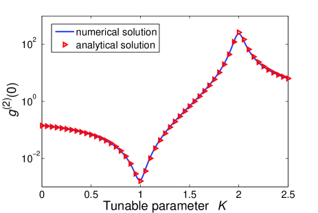
Figure 5: (Color online). The numerical and analytical solutions for the second-order correlation function $g^{(2)}(0)$ in Eq. (25) versus the tunable parameter ${K}$. The system parameters for this simulation are: $\chi=10$ MHz, $\Delta_{s}=50$ MHz, $\gamma/2\pi=2$ MHz, $\gamma_{f}/2\pi=2.5$ MHz, $\kappa=1$ MHz, and $\varepsilon=0.1\kappa$.

We compare the numerical and analytical solutions of ${g}^{(2)}(0)$ in Fig. 5. The analytical solution of $g^{\left(2\right)}\left(0\right)$ is obtained in the following way. From Eq. (25), we have Xu

$$g^{(2)}(0)=\frac{\sum\limits_{n}n(n-1)P_{n}}{\left(\sum\limits_{n}nP_{n}\right)^{2}},$$ (26)

where $P_{n}$ represents the probability with $n$ photons. In the weak-driving limit, i.e., $\varepsilon\to 0$, it can be shown that $P_{n}\gg P_{n+1}$ for $n\geq 2$. Thus, we can omit the probability for three or more photons. In this case, the steady state of the system can be expressed as:

$$\left|\psi\right\rangle=\sum\limits_{n_{p}=0}^{2}\sum\limits_{n_{c}=0}^{2}C_{n_{p},n_{c}}\left|n_{p},n_{c}\right\rangle,$$ (27)

where $\left|n_{p}\right\rangle$ and $\left|n_{c}\right\rangle$ are the states of the controlled system and the controller respectively. In order to find the coefficients $C_{n_{p},n_{c}}$ for the steady state, we introduce the complex Hamiltonian by letting

$$\Delta_{s}\to\Delta_{s}-i(\sqrt{\gamma}+\sqrt{\gamma}_{f})^{2}/2,$$

$$\Delta\to\Delta-i\kappa/2$$

to represent the dissipation effects. Then, the steady state can be found via ${\rm d}\left|\psi(t)\right\rangle/{\rm d}t=0$. The probability of the $n_{p}$-th occupation number can be expressed as

$$P_{n_{p}}=\sum\limits_{n_{c}}\left|C_{n_{p},n_{c}}\right|^{2}.$$

Thus, in the weak-driving limit, $g^{(2)}(0)$ can be described by (see derivations in Appendix B)

$$g^{(2)}(0)=\frac{\left|\Delta_{s}+(K-2)\chi-\frac{i}{2}\gamma_{a}\right|^{2}\left|(K-1)\chi-\frac{i}{2}\kappa\right|^{2}}{\left|\left((K-2)\chi-\frac{i}{2}\kappa\right)\left(\Delta_{s}+(K-1)\chi-\frac{i}{2}\gamma_{a}\right)\right|^{2}},$$ (28)

with

$$\gamma_{a}=(\sqrt{\gamma}+\sqrt{\gamma}_{f})^{2}+\kappa.$$

In Fig. 5, the analytical result for $g^{(2)}(0)$ fits well with the numerical solution obtained by the few photon truncation in the weak-driving regime. It can be shown that

$$g^{(2)}(0)=\frac{4\kappa^{2}\left(\Delta_{s}-\chi\right)^{2}+\kappa^{2}\gamma_{a}^{2}}{4\kappa^{2}\Delta_{s}^{2}+16\chi^{2}\Delta_{s}^{2}+\left(4\chi^{2}+\kappa^{2}\right)\gamma_{a}^{2}},$$ (29)

when $K=1$. When the dissipation coefficients $\kappa$, $\gamma$, and $\gamma_{f}$ are far less than the Kerr nonlinear coefficient $\chi$ and the detunning frequency $\Delta_{s}$, we have $g^{(2)}(0)<1$ which leads to the single-photon blockade.

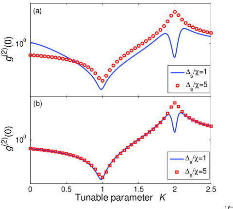
Figure 6: (a) $g^{(2)}(0)$ for the controlled TLR and (b) $g^{(2)}(0)$ for the controller versus the parameter $K=\Delta/\chi+1$. The red dotted curve and the blue curve correspond to different detuning frequencies $\Delta_{s}=50$ MHz and $\Delta_{s}=10$ MHz. The other system parameters are: $\chi=10$ MHz $\gamma/2\pi=2$ MHz, $\gamma_{f}/2\pi=2.5$ MHz, $\kappa=1$ MHz, and $\varepsilon=0.1\kappa$.

We plot the curve of $g^{(2)}(0)$ for the controlled single-mode cavity in the TLR in Fig. 6(a). We find that there is a minimum point of $g^{(2)}(0)$ at $K=1$ for each curve, which means that photon antibunching occurs. This typical nonlinear quantum phenomenon observed in the linear-controlled single-mode cavity in the TLR is induced by the Kerr nonlinearity in the controller by coherent feedback.

However, the curves for different detuning frequencies $\Delta_{s}$ are different at $K=2$. For $\Delta_{s}/\chi=1$, we can observe that $g^{\left(2\right)}\left(0\right)<1$ which means that photon blockade occurs. In this case, it can be shown from $K=2$ and $\Delta_{s}/\chi=1$ that $\omega_{s}=\omega_{c}$, which means that the controller and the controlled TLR resonate with each other. When the resonance occurs, if one photon enters the controlled TLR, this photon will be transmitted to the controller from the feedback loop and then transmitted back. It will block the next photon to enter the controlled TLR. In Fig. 6(b), we can find for the curve with $\Delta_{s}/\chi=5$ that $g^{\left(2\right)}\left(0\right)>1$ at $K=2$, which means two photons resonating. This corresponds to a transparency effect.

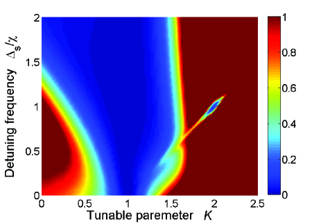
Figure 7: (Color online). Second-order correlation function versus $K$ and $\Delta_{s}$, with $\chi=10$ MHz, $\gamma/2\pi=2$ MHz, $\gamma_{f}/2\pi=2.5$ MHz, $\kappa=1$ MHz and $\varepsilon=0.1\kappa$. Note that $g^{(2)}(0)<1$ occurs when $\Delta_{s}-(K-1)=0$, namely, $\omega=\omega_{s}$ and $K=1$ with any $\Delta_{s}$.

In Fig. 7, we show how $g^{(2)}(0)$ depends on the parameters $K$ and $\Delta_{s}$. The photon antibunching occurs at $K=1$ with any $\Delta_{s}$. However, at $K=2$ it can only be observed when $\Delta_{s}/\chi=1$, which means that the controlled TLR and the controller are resonant with each other.

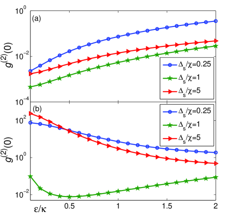
Figure 8: (Color online). Second-order correlation function versus the normalized driving strength $\varepsilon/\kappa$, for different values of the detuning frequency $\Delta_{s}$. Here the system parameters are: $\chi=10$ MHz, $\gamma/2\pi=2$ MHz, $\gamma_{f}/2\pi=2.5$ MHz, and $\kappa=1$ MHz. (a) for $K=1$ and (b) for $K=2$.

In Fig. 8, we also study how $g^{(2)}(0)$ depends on the strength of the driving field. In Fig. 8(a), we find that $g^{(2)}(0)\to 1$ when increasing the strength of the driving field. We can also observe that $g^{(2)}(0)$ is minimized when the resonance occurs, i.e., $\Delta_{s}/\chi=1$. Similar to Fig. 8(a), in Fig. 8(b) we find that all the curves converge to $1$ when increasing the strength of the driving field. However, we can obtain a concave curve when the resonance occurs, i.e., $\Delta_{s}/\chi=1$.

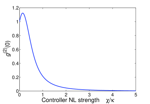
Figure 9: (Color online). Second-order correlation function versus the nonlinear strength $\chi$ of the controller, where the parameters of the system are: $K=1$, $\gamma/2\pi=2\ \rm MHz$, $\gamma_{f}/2\pi=2.5$ MHz, $\kappa=1$ MHz and $\varepsilon=0.1\kappa$.

The generated nonlinear effects in the controlled single-mode field in the TLR can be enhanced by increasing the nonlinear strength of the controller, and the nonlinear strength $\chi$ of the controller can be tuned by adjusting the detuning frequency $\Delta_{qT}$. Thus, we can enhance the generated nonlinear effects in the controlled TLR by tuning $\Delta_{qT}$. Indeed, from Fig. 9, we can find that the antibuching effects in the controlled TLR are enhanced by decreasing the detuning $\Delta_{qT}$.

VI Conclusions

In summary, we presented a nonlinear coherent feedback-control system in superconducting circuits in which a controlled linear transmission line resonator is modulated by another transmission line resonator coupled to a dc-SQUID-based superconducting charge qubit in the feedback loop. Such a design changes the linear dynamics of the controlled resonator and makes it nonlinear. This nonlinear coherent feedback-control system is used to produce strong nonlinear on-chip optical phenomena. In the semiclassical regime, we observe in simulations bistable optical-type phenomena observed in previous optical experiments, and give the condition to observe this bistability.

In the quantum regime, we predict a photon antibunching induced by nonlinear coherent feedback, which is believed to be a typical quantum optics phenomenon that violates the Cauchy-Schwartz inequality for classical light. Our study shows that dynamics of linear system can be switched to nonlinear one by using nonlinear coherent feedback in a controllable way. We hope that our prediction of nonlinear coherent feedback in the quantum regime can be verified experimentally in the near future.

ACKNOWLEDGMENTS

ZPL would like to thank Dr. X.W. Xu for helpful discussions. JZ and RBW are supported by the NSFC under Grant Nos.61174084, 61134008, 60904034, and project supported by State Key Laboratory of Robotics, Shenyang Institute of Automation Chinese Academy of Sciences, China. YXL is supported by the NSFC under Grant Nos. 61025022, 60836001. FN is partially supported by the ARO, RIKEN iTHES Project, MURI Center for Dynamic Magneto-Optics, JSPS-RFBR contract No.12-02-92100, Grant-in-Aid for Scientific Research (S), MEXT Kakenhi on Quantum Cybernetics, and the JSPS via its FIRST program.

Appendix A qubit-induced nonlinearity

If the detuning frequency $\Delta_{qT}=\omega_{c}-\omega_{0}$ between the qubit and the TLR is much lager than the intensity $g$ between the qubit and the TLR, by making the unitary transformation

$$U_{0}=\exp\left[\frac{g}{\Delta_{qT}}\left(c\sigma_{+}-c^{{\dagger}}\sigma_{-}\right)\right],$$ (30)

the effective Hamiltonian can be described as

$$H_{\rm eff} =U_{0}HU_{0}^{{\dagger}}$$ (31)

$$\approx\left(\omega_{c}+\frac{g^{2}}{\Delta_{qT}}\sigma_{z}\right)c^{{\dagger}}c+\frac{1}{2}\left(\omega_{0}+\frac{g^{2}}{\Delta_{qT}}\right)\sigma_{z}$$

$$+\Omega\left(\sigma_{+}e^{-i\omega_{1}t}+\sigma_{-}e^{i\omega_{1}t}\right)$$

In the rotating reference frame with frequency $\omega_{1}$ of the driving field, we let

$$U_{1}=\exp\left[-i\omega_{1}\frac{\sigma_{z}}{2}\right]t$$ (32)

where $\omega_{1}=\omega_{0}+\frac{g^{2}}{\Delta_{qT}}$, the Hamiltonian can then be described by

$$H_{\rm eff}^{\prime}=\omega_{c}c^{{\dagger}}c+\Omega\sigma_{x}+\frac{g^{2}}{\Delta_{qT}}c^{{\dagger}}c\sigma_{z}$$ (33)

We set $\sigma_{z}\rightarrow\sigma_{x}$, and then

$$H_{\rm eff}^{\prime\prime}=\omega_{c}c^{{\dagger}}c+\Omega\sigma_{z}+\frac{g^{2}}{\Delta_{qT}}c^{{\dagger}}c\left(\sigma_{+}+\sigma_{-}\right).$$ (34)

If the Rabi frequency $\Omega$ satisfies the condition $\Omega\gg(g^{2}/\Delta_{qT})$, through the unitary transformation

$$U_{2}=\exp\left[\frac{g^{2}}{2\Omega\Delta_{qT}}c^{{\dagger}}c\left(\sigma_{+}-\sigma_{-}\right)\right],$$ (35)

the Hamiltonian can be re-expressed by

$$H_{\rm eff}^{\prime\prime\prime}=\omega_{c}c^{{\dagger}}c+\Omega\sigma_{z}+\frac{g^{4}}{2\Omega\Delta_{qT}^{2}}\left(c^{{\dagger}}c\right)^{2}\sigma_{z}.$$ (36)

Appendix B Derivation of the second-order correlation for the controlled system

In the limit of a weak driving field, the state $|\psi\rangle$ can be derived using perturbation theory. In order to show explicitly the second-order correlation, up to second order in $|\varepsilon|$, we set $|\psi\rangle=C_{00}|00\rangle+C_{01}|01\rangle+C_{02}|02\rangle+C_{10}|10\rangle+C_{11}|11\rangle+C_{12}|12\rangle+C_{20}|20\rangle+C_{21}|21\rangle+C_{22}|22\rangle$. The steady solution for the coefficients $C_{{n_{a}}{n_{c}}}$ can be given by the Schrödinger equation for $|\psi\rangle$, when the limit of neglecting pure dephasing is neglected,

$$i\frac{{\rm d}|\psi\rangle}{{\rm d}t}=H_{\rm tot}|\psi\rangle,$$ (37)

assuming ${\rm d}\left|\psi(t)\right>/{\rm d}t=0$ , and

$$0=\Delta_{s}C_{10}-\varepsilon C_{11}+\frac{i}{2}\left(\sqrt{\kappa\gamma}-\sqrt{\kappa\gamma_{f}}\right)C_{01},$$ (38)

$$0=\Delta_{s}C_{10}-\varepsilon C_{11}+\frac{i}{2}\left(\sqrt{\kappa\gamma}-\sqrt{\kappa\gamma_{f}}\right)C_{01},$$ (39)

$$0= \left(\Delta_{s}+\Delta\right)C_{11}-\varepsilon C_{10}-\sqrt{2}\varepsilon C_{12}$$ (40)

$$+\frac{i}{\sqrt{2}}\left(\sqrt{\kappa\gamma}-\sqrt{\kappa\gamma_{f}}\right)C_{02}-\frac{i}{\sqrt{2}}(\sqrt{\kappa\gamma}-\sqrt{\kappa\gamma_{f}})C_{20},$$

$$0= \left(\Delta_{s}+2\Delta-2\chi\right)C_{12}-\sqrt{2}\varepsilon C_{11}$$ (41)

$$-i\left(\sqrt{\kappa\gamma}-\sqrt{\kappa\gamma_{f}}\right)C_{21},$$

$$0= -\varepsilon C_{00}-\sqrt{2}\varepsilon C_{02}-\frac{i}{2}\left(\sqrt{\kappa\gamma}-\sqrt{\kappa\gamma_{f}}\right)C_{10}+\Delta C_{01},$$ (42)

$$0= \left(2\Delta-2\chi\right)C_{02}-\sqrt{2}\varepsilon C_{01}-\frac{i}{\sqrt{2}}(\sqrt{\kappa\gamma}-\sqrt{\kappa\gamma_{f}})C_{11},$$ (43)

$$0= \left(2\Delta_{s}+\Delta\right)C_{21}-\varepsilon C_{20}-\sqrt{2}\varepsilon C_{22}$$ (44)

$$+i\left(\sqrt{\kappa\gamma}-\sqrt{\kappa\gamma_{f}}\right)C_{12},$$

$$0= 2\Delta_{s}C_{20}-\varepsilon C_{21}+\frac{i}{\sqrt{2}}\left(\sqrt{\kappa\gamma}-\sqrt{\kappa\gamma_{f}}\right)C_{11},$$ (45)

$$0= \left(2\Delta_{s}+2\Delta-2\chi\right)C_{22}-\sqrt{2}\varepsilon C_{21}.$$ (46)

Due to the weak limit of the driving field, we can assume $C_{00}\to 1$. And the equations are now closed (i.e., nine equations for nine parameters). Thus, it is possible to obtain the analytical solution of the system. However, the solution is cumbersome, but we can neglect the higher order terms in $|\varepsilon|$, obtaining

$$P_{1}= |C_{10}|^{2}+|C_{11}|^{2}+|C_{12}|^{2}\approx \frac{|\left(\sqrt{\kappa\gamma}-\sqrt{\kappa\gamma_{f}}\right)\varepsilon|^{2}}{|\left(\Delta-\chi\right)\Delta_{s}|^{2}}$$ (47)

$$P_{2}= |C_{20}|^{2}+|C_{21}|^{2}+|C_{22}|^{2}$$ (48)

$$\approx \frac{|\left(\sqrt{\kappa\gamma}-\sqrt{\kappa\gamma_{f}}\right)\varepsilon|^{4}|\Delta_{s}-2\chi+\Delta|^{2}}{2|\left(\Delta-\chi\right)\left(\Delta-2\chi\right)\left(\Delta_{s}+\Delta-\chi\right)\Delta_{s}^{2}|^{2}}$$

We substitute Eqs. (47)(48) into Eq. (26), and then we can derive the analytical solution of the $g^{(2)}(0)$ in the form of Eq.(28).

References

- (1) K. J. Åström and R.M. Murray, Feedback Systems: An Introduction for Scientists and Engineers (Princeton University Press, Princeton, NJ, 2008).
- (2) H. M. Wiseman and G. J. Milburn, Quantum Measurement and Control (Cambridge University Press, Cambridge, England, 2009).
- (3) D. Y. Dong and I. R. Petersen, IET Control Theory and Applications 4, 2651 (2010).
- (4) C. Altafini and F. Ticozzi, IEEE Trans. Automat. Contr. 57, 1898 (2012).
- (5) J. Kerckhoff, R. W. Andrews, H. S. Ku, W. F. Kindel, K. Cicak, R. W. Simmonds, and K. W. Lehnert, Phys. Rev. X 3, 021013 (2013).
- (6) V. P. Belavkin, J. Multivariate Anal. 42, 171 (1992); Commun. Math. Phys. 146, 611 (1992); Theor. Probab. Appl. 38, 573 (1993).
- (7) H. M. Wiseman and G. J. Milburn, Phys. Rev. A 49, 1350 (1994).
- (8) J. E. Gough and S. Wildfeuer, Phys. Rev. A 80, 042107 (2009).
- (9) S. Iida, M. Yukawa, H. Yonezawa, N. Yamamoto, and A. Furusawa, IEEE Trans. Automat. Contr. 57, 2045 (2012).
- (10) L. K. Thomsen, S. Mancini, and H. M. Wiseman, Phys. Rev. A 65, 061801 (2002).
- (11) J. Wang and H. M. Wiseman, Phys. Rev. A 64, 063810 (2001).
- (12) J. K. Stockton, R. van Handel, and H. Mabuchi, Phys. Rev. A 70, 022106 (2004).
- (13) R. van Handel, J. K. Stockton, and H. Mabuchi, IEEE Trans. Automat. Contr. 50, 768 (2005).
- (14) P. Campagne-Ibarcq, E. Flurin, N. Roch, D. Darson, P. Morfin, M. Mirrahimi, M. H. Devoret, F. Mallet, and B. Huard, Phys. Rev. X 3, 021008 (2013).
- (15) D. Vitali, P. Tombesi, and G. J. Milburn, Phys. Rev. A 57, 4930 (1998).
- (16) N. Ganesan and T.-J. Tarn, Phys. Rev. A 75, 032323 (2007).
- (17) J. Zhang, R.-B. Wu, C.-W. Li, and T.-J. Tarn, IEEE Trans. Automat. Contr. 55, 619 (2010).
- (18) G. F. Zhang and M. R. James, IEEE Trans. Automat. Contr. 56, 1535 (2011).
- (19) B. Qi and L. Guo, Sys. Contr. Lett. 59, 333 (2010).
- (20) R. Vijay, C. Macklin, D. H. Slichter, S. J. Weber, K. W. Murch, R. Naik, A. N. Korotkov and I. Siddiqi, Nature 490, 77 (2012).
- (21) C. Ahn, A. C. Doherty, and A. J. Landahl, Phys. Rev. A 65, 042301 (2002); J. Kerckhoff, H. I. Nurdin, D. S. Pavlichin, and H. Mabuchi, Phys. Rev. Lett. 105, 040502 (2010).
- (22) S.-B. Xue, R.-B. Wu, W.-M. Zhang, J. Zhang, C.-W. Li, and T.-J. Tarn, Phys. Rev. A 86, 052304 (2012).
- (23) J. Wang, H. M. Wiseman, and G. J. Milburn, Phys. Rev. A 71, 042309 (2005).
- (24) N. Yamamoto, K. Tsumura and S. Hara, Automatica, 43, 981 (2007).
- (25) Z. Liu, L. L. Kuang, K. Hu, L. T. Xu, S. H. Wei, L. Z. Guo, and X. Q. Li, Phys. Rev. A 82, 032335 (2010).
- (26) A. Hopkins, K. Jacobs, S. Habib, and K. C. Schwab, Phys. Rev. B 68, 235328 (2003).
- (27) J. Zhang, Y.-X. Liu, and F. Nori, Phys. Rev. A 79, 052102 (2009).
- (28) Ya. S. Greenberg, E. Il ichev, and F. Nori, Phys. Rev. B 80, 214423 (2009); K. Xia and J. Evers, Phys. Rev. B 82, 184532 (2010).
- (29) M. J. Woolley, A. C. Doherty, and G. J. Milburn, Phys. Rev. B 82, 094511 (2010).
- (30) J. Combes and K. Jacobs, Phys. Rev. Lett. 96, 010504 (2006). J. Combes, H. M. Wiseman, and K. Jacobs, Phys. Rev. Lett. 100, 160503 (2008).
- (31) J. Zhang, Y.-X. Liu, R.-B. Wu, C.-W. Li, and T.-J. Tarn, Phys. Rev. A 82, 022101 (2010).
- (32) H. M. Wiseman and G. J. Milburn, Phys. Rev. Lett. 70, 548 (1993); H. M. Wiseman, Phys. Rev. A 49, 2133 (1994).
- (33) H. Mabuchi and A. C. Doherty, Science 298, 1372 (2002).
- (34) A. C. Doherty, S. Habib, K. Jacobs, H. Mabuchi, and S. M. Tan, Phys. Rev. A 62, 012105 (2000).
- (35) S. Mancini, Phys. Rev. A 73, 010304(R) (2006).
- (36) H. M. Wiseman and G. J. Milburn, Phys. Rev. A 49, 4110 (1994).
- (37) S. Lloyd, Phys. Rev. A 62, 022108 (2000).
- (38) M. R. James, H. I. Nurdin, and I. R. Petersen, IEEE Trans. Automat. Contr. 53, 1787 (2008).
- (39) M. Yanagisawa, H. Kimura, IEEE Trans. Automat. Contr. 48, 2107 (2003).
- (40) J. Gough and M. R. James, IEEE Trans. Automat.Contr. 54, 2530 (2009).
- (41) D. Riste, C. C. Bultink, K. W. Lehnert, and L. DiCarlo, Phys. Rev. Lett. 109, 240502 (2012).
- (42) F. Sciarrino, M. Ricci, F. De Martini, R. Filip, and L. Mišta, Jr., Phys. Rev. Lett. 96, 020408 (2006).
- (43) S. Brakhane, W. Alt, T. Kampschulte, M. M. Dorantes, R. Reimann, S. Yoon, A. Widera, and D. Meschede, Phys. Rev. Lett. 109, 173601 (2012).
- (44) H. Yonezawa, D. Nakane, T. A. Wheatley, K. Iwasawa, S. Takeda, H. Arao, K. Ohki, K. Tsumura, D. W. Berry, T. C. Ralph, H. M. Wiseman, E. H. Huntington, and A. Furusawa, Science 337, 1514 (2012).
- (45) J. Gieseler, B. Deutsch, R. Quidant, and L. Novotny, Phys. Rev. Lett. 109, 103603 (2012).
- (46) D. W. Berry and H. M. Wiseman, Phys. Rev. Lett. 85, 5098 (2000).
- (47) A. Kubanek, M. Koch, C. Sames, A. Ourjoumtsev, P. W. H. Pinkse, K. Murr and G. Rempe, Nature 462, 898 (2009).
- (48) C. Sayrin, I. Dotsenko, X. Zhou, B. Peaudecerf, T. Rybarczyk, S. Gleyzes, P. Rouchon, M. Mirrahimi, H. Amini, M. Brune, J. M. Raimond, and S. Haroche, Nature 477, 73 (2011).
- (49) X. Zhou, I. Dotsenko, B. Peaudecerf, T. Rybarczyk, C. Sayrin, S. Gleyzes, J. M. Raimond, M. Brune, and S. Haroche, Phys. Rev. Lett. 108, 243602 (2012).
- (50) R. J. Nelson, Y. Weinstein, D. Cory, and S. Lloyd, Phys. Rev. Lett. 85, 3045 (2000).
- (51) H. Mabuchi, Phys. Rev. A 78, 032323 (2008).
- (52) Z .F. Zhou, C. J. Liu, Y. M. Fang, J.Zhou, R. T. Glasser, L. Q. Chen, J. T. Jing, and W. P. Zhang, Appl. Phys. Lett. 101, 191113 (2012).
- (53) J. Kerckhoff, and K. W. Lehnert, Phys. Rev. Lett. 109, 153602 (2012).
- (54) S. Iida, M. Yukawa, H. Yonezawa, N. Yamamoto, and A. Furusawa, IEEE Trans. Automat. Contr. 57, 2045 (2012).
- (55) D. Jaksch, C. Bruder, J. I. Cirac, C. W. Gardiner, and P. Zoller, Phys. Rev. Lett. 81, 3108 (1998).
- (56) K. M. Birnbaum, A. Boca, R. Miller, A. D. Boozer, T. E. Northup, and H. J. Kimble, Nature 436, 87 (2005).
- (57) J. M. Fink, M. Goppl, M. Baur, R. Bianchetti, A. Leek,P. J. Blais, and A. Wallraff, Nature 454, 315 (2008).
- (58) L. S. Bishop, J. M. Chow, J. Koch, A. A. Houck, M. H. Devoret, E. Thuneberg, S. M. Girvin, and R. J. Schoelkopf, Nat. Phys. 5, 105 (2009).
- (59) A. Politi, J.C.F. Matthews, and J. L. O’Brien, Science 325, 1221 (2009).
- (60) J.C.F. Matthews, A. Politi, A. Stefanov, and J. L. O’Brien, Nat. Photonics 3, 346 (2009).
- (61) D. W. Berry and H. M. Wiseman, Nat. Photonics 3, 317 (2009).
- (62) J. Zhang, R.-B. Wu , Y.-X. Liu, C.-W Li, and T.-J. Tarn, IEEE Trans. Automat. Contr. 57, 1997 (2012).
- (63) J. Q. You, Y.-X. Liu, C. P. Sun, and F. Nori, Phys. Rev. B 75, 104515 (2007).
- (64) A. J. Hoffman, S.J. Srinivasan, S. Schmidt, L. Spietz, J. Aumentado, H. E. Türeci, and A. A. Houck, Phys. Rev. Lett. 107, 053602 (2010).
- (65) P. D. Nation, and M. P. Blencowe, E. Buks, Phys. Rev. B 78, 104516 (2008).
- (66) I. Tornes, and D. Stroud, Phys. Rev. B 77, 224513 (2008).
- (67) I. Buluta, S. Ashhab, and F. Nori, Rep. Prog. Phys. 74, 104401 (2011).
- (68) I. Georgescu, and F. Nori, Phys. World 25, 16-17 (2012).
- (69) I. Buluta, and F. Nori, Science 326, 108-111 (2009).
- (70) P. D. Nation, J. R. Johansson, and M. P. Blencowe, and F. Nori, Rev. Mod. Phys. 84, 1-24 (2012).
- (71) J. Q. You, and F. Nori, Phys. Today 58, 42-47 (2005).
- (72) J. Q. You, and F. Nori, Nature 474, 589 (2011).
- (73) Z.-L. Xiang, S. Ashhab, J. Q. You, and F. Nori, Rev. Mod. Phys. 85, 623 (2013).
- (74) C. W. Gardiner and M. J. Collett, Phys. Rev. A 31, 3761 (1985); C. W. Gardiner and P. Zoller, Quantum Noise (Springer-Verlag, Berlin, 2004) (3rd edition).
- (75) A detailed and pedagogical derivation of the input-output formalism can be found in: K. Jacobs, PhD dissertation, Imperial, London, Eprint:arXiv:quant-ph/9810015.
- (76) G. Wendin and V. S. Shumeiko, Handbook of Theoretical and Computational Nanotechnology edited by M. Rieth and W. Schommers (ASP, Los Angeles, 2006), Vol. 3, pp. 223 C309.
- (77) M. A. Castellanos-Beltran, K. D. Irwin, G. C. Hilton, L. R. Vale, and K. W. Lehnert, Nature phys. 4, 929 (2008).
- (78) Y.-X. Liu, A. Miranowicz, Y. B. Gao, J. Bajer, C. P. Sun, and F. Nori, Phys. Rev. A 82, 032101 (2010).
- (79) H. M. Gibbs, S. L. McCall, and T. N. C. Venkatesan, Phys. Rev. Lett. 36, 1135 (1976).
- (80) G. Rempe, R. J. Thompson, R. J. Brecha, W. D. Lee, and H. J. Kimble, Phys. Rev. Lett. 67, 1727 (1991).
- (81) A. Sauer, K. M. Fortier, M. S. Chanf, C. D. Hamley, and M. S. Chapman, Phys. Rev. A 69, 051804 (2004).
- (82) S. Gupta, K. L. Moore, K. W. Murch, and D. M. Stamper-Kurn, Phys. Rev. Lett. 99, 213601 (2007).
- (83) F. Brennecke, S. Ritter, T. Donner, and T. Esslinger, Science 322, 235 (2008).
- (84) Y. F Xiao, Ş. K. Özdemir, V. Gaddam, C. H. Dong, N. Imoto, and L. Yang, Opt. Express 16, 21462 (2008).
- (85) H. Wang, H. C. Sun, J. Zhang, and Y.-X. Liu, Science China 55, 2264 (2012).
- (86) R. R. Puri, Mathematical Methods of Quantum Optics (Springer-Verlag, Berlin, 2001).
- (87) A. Miranowicz, M. Paprzycka, Y.-X. Liu, J. Bajer, and F. Nori, Phys. Rev. A 87, 023809 (2013).
- (88) X. W. Xu, and Y. J. Li, J. Phys. B: At. Mol. Opt. Phys. 46, 035502 (2013).