Newton-like equations for a radiating particle

Abstract

Second order Newton equations of motion for a radiating particle are presented. It is argued that the trajectories obeying them also satisfy the Abraham-Lorentz-Dirac (ALD) equations for general 3D motions in the non-relativistic and relativistic limits. The case of forces only depending of the proper time is here considered. For these properties to hold, it is sufficient that the external force to be infinitely smooth and that a series formed with its time derivatives converges. This series define in a special local way the effective forces entering the Newton equations. When the external force vanishes in an open vicinity of a given time, the effective one also becomes null. Thus, the proper solutions of the effective equations can not show runaway or pre-acceleration effects. The Newton equations are numerically solved for a pulsed force given by an analytic function along the proper time axis. The simultaneous satisfaction of the ALD equations is numerically checked. Further, a set of modified ALD equations for almost everywhere infinitely smooth forces, but including step like discontinuities in some points is also presented for the case of collinear motions. The form of the equations supports the statement argued in a previous work, about that the causal Lienard-Wiechert field solution surrounding a radiating particle, implies that the effective force on the particle should instantaneously vanish when the external force is retired. The modified ALD equations proposed in the previous work are here derived in a generalized way including the same effect also when a the force is instantly connected.

A. Cabo E-Mail: cabo@icimaf.cu
 N. G .Cabo Bizet  E-Mail: nana@ceaden.edu.cu

I Introduction

The long-standing search for a consistent formulation of the Abraham-Lorentz-Dirac equation (ALD) for a radiating particle remains being a field of intense research activity Lorentz ; abraham ; poincare ; schot ; Dirac ; Teitelboim ; Landau ; Rohrlich ; Yighjian ; Ford ; Spohn ; Raju . The complete understanding of the formulation and solution of the equations had presented hard theoretical difficulties. The existence of solutions with values growing without bound (runaway behavior) or pre-accelerated motions in advance to the applied forces, are two of the most debated issues associated to the ALD equations Yighjian ; Spohn . Important advances in the understanding of these properties had been by now obtained in Refs. Yighjian ; Ford . In particular, in Ref. Yighjian , it was argued that the ALD equations can’t be derived in a completely exact way from the integral equations satisfied by the coupled motion of a particle and its accompanying electromagnetic field for non analytically depending forces.  Moreover, the author derived a correction to the ALD equations which should be used in order to consider suddenly changing forces. The change corresponded to multiplying the reaction force of the field on the particle by a proper-time dependent function $\ \eta(\tau)$ which vanish at the proper time value at which the forces is started to be applied, and attains a unit value in a small time interval of the order of the time required by light to travel the radius of the considered structured body studied in Ref. Yighjian . This change was argued to allow eliminating both: the runaway and the pre-accelerated types of solutions. Thus, in general terms, it was concluded that the ALD equations are not exact consequences of the integral equations of motions for the coupled system describing the structured particle investigated in Ref. Yighjian . In addition, in Refs Ford , the authors presented a derivation of a simpler second order in the time derivative of the position, for a radiating particle, assuming that it shows an internal structure. The equation derived was argued to be exact for the structured particle, which could justify its incomplete equivalence with the ALD equation Ford .

In the present work, at variance with the studies in Refs. Yighjian ; Ford we will not consider that the radiating particles has a structure.  Our work, is rather devoted to identify and study some properties of a curious second order Newton type of equation motion for the radiating particle, that when satisfied, by assuming that the force is a infinitely smooth function, directly obey the ALD equations. This occurs in a proper time region of convergence of a particular series conformed with the infinite sequence of the time derivatives of the force at a given instant. The effective force at this instant results to be defined by the local values of the series at that moment, which implies that the effective force vanishes when the external one is null within an open neighborhood, which eliminates the possibility of pre-acceleration of runway solutions when the external force vanishes.   To motivate the second order equations, firstly we present their equivalence with the ALD ones in the non-relativistic version of them for a general 3D motion. Next, the equations are generalized to the relativistic case by a simple construction. The work also presents the solution of the equations for a simple example of a pulse like force for which the above mentioned particular series of their proper time derivatives converge in the whole time axis. The effective force is evaluated, and the position, velocity, acceleration and its derivative, are determined from the numerical solution of the equations. The results does not show runaway or pre-accelerated behaviors, since as noted before, the effective force only depends on the local behavior around a proper time instant. The case of forces being infinitely smooth, but eventually showing a numerable set of step like discontinuities is also analyzed for the case in which the motion is collinear. It becomes possible to derive modified ALD equation of motion, after assuming that, as in the example of the analytic pulse, the discontinuous force can be expressed as the limit of a sequence of infinitely smooth forces, which define a corresponding sequence of effective forces also showing the same kind of discontinuity as the external one in the limit. The modified ALD equations give a generalization of the ones derived in reference cabojorge and fully support the central idea proposed in that work: that the validity of the Lienard-Wiechert solutions for the electromagnetic field closely around the particle,  just after the external forces is retired, implies that its acceleration should also suddenly disappears. This is a natural consequence of the fact that the electromagnetic field in a sufficiently close small vicinity of the particle is given by a Lorentz boosted Coulomb field, which is known to not produce any force on the central particle. Using these modified equations we also investigated their solutions for an external force in the form of a rigorously squared pulse which exactly vanishes outside a given time interval. An important point to stress is that the Delta function like terms within the smooth solution for the squared pulse obtained, follow as ”normal” contributions to the usual ”radiation” force terms. Thus, their presence is consistent with the well understood notion about that the ALD equation well describe the radiation properties of a moving particle. However, in addition it also follows that such Delta function terms exactly cancel with other ones associated to time derivatives of step like changes in the acceleration occurring at the discontinuities. This means that, effectively, the discontinuities, do not contribute with finite terms to the radiation, contrary to what could be expected due to the appearance of the Delta functions in the modified equations.

The expositions proceed as follows. In section 2, the Newton like equation which solutions also satisfy the non-relativistic ALD equations for a general 3D dynamics is presented. Section 3, generalizes the discussion by constructing a relativist Newton like equation which also satisfies the relativistic ALD one.  Next, Section 4 presents concrete conditions which determine that given an infinitely smooth external force, the effective force determined by it, becomes also well defined. Section 5 continues by presenting the numerical solution of the Newton second order equations for the case of a force being similar to a squared pulse, but being defined by an analytical function along all the time axis. The following Section 6 is devoted to derive the modified ALD equations for forces defined almost everywhere by infinitely smooth functions, but which show step like discontinuities at a denumerable set of instants along the time axis. In Section 7, the modified ALD equations are solved for the rigorous squared pulse. This force pertains to the class of almost everywhere $C^{\infty}$ functions, showing step like discontinuities. The solution is compared with the one associated to the previously studied analytical pulsed force. They show a very close appearance, indicating the presence of Dirac delta functions concentrated at the discontinuity points of the external force in the modified ALD equations. Finally, in the summary the results are shortly reviewed and possible extensions of the work commented.

II The case of the non-relativistic ALD equations

Let us consider a general but nonrelativistic motion of a particle $P$ along a space-time trajectory $C$ defined by a curve $x$($\tau)=(x^{1}(t),\,x^{2}(t),\,x^{3}(t))$ and parameterized by the time $t.$  For this motion, the non-relativistic ALD equations take the standard form

$$m\text{ }a^{i}(t)-f^{i}(t)\text{\ } \text{=}\,\kappa\text{ }\frac{da^{i}(t)}{dt}\text{ },$$ (1)

$$v^{i}(t)\text{ } \text{=\ }\overset{\cdot}{x}^{i}(t)\text{ =}\frac{dx^{i}(t)}{dt}\text{\ ,}$$ (2)

$$a^{i}(t)\text{ } \text{=\ }\overset{\cdot}{v}^{i}(t)\text{ =}\frac{dv^{i}(t)}{dt}\text{\ ,}$$ (3)

where the index $i$ has the three values $i=1,2,3$.  In what follows, without attempting to repeat the trial and error process which led to the mentioned solution, we will directly write its expression for afterwards arguing that it solves the above equations (1).

The second order Newton-like equations have the specific form

$$a^{i}(t)=\frac{1}{m}\sum_{n=0}^{\infty}\frac{d^{n}}{dt^{n}}f^{i}(t)(\frac{\kappa}{m})^{n}.$$ (4)

Let us assume that the forces are infinitely smooth, that is, pertaining to $C^{\infty}$ and that the series at the right hand side (r.h.s) converges in certain interval of times. Then, for the time derivative of the acceleration we have

$$\overset{\cdot}{a}^{i}(t) =\frac{1}{m}\sum_{n=0}\frac{d^{n+1}}{dt^{n+1}}f^{i}(t)(\frac{\kappa}{m})^{n}$$

$$=\frac{1}{\kappa}\sum_{n=0}\frac{d^{n+1}}{dt^{n+1}}f^{i}(t)(\frac{\kappa}{m})^{n+1}$$

$$=\frac{1}{\kappa}(\sum_{n=0}\frac{d^{n}}{dt^{n}}f^{i}(t)(\frac{\kappa}{m})^{n}-f^{i}(t))$$

$$=\frac{1}{\kappa}(m\text{ }a^{i}(t)-f^{i}(t)),$$ (5)

where, as before, in the following a point over a quantity will mean a derivative over the defined temporal argument of it. Therefore, assumed that the series is well defined, the trajectory $x^{i}(t)$  solving equation (4), also satisfies the non-relativistic ALD equations

$$m\text{ }a^{i}(t)-f^{i}(t)=\kappa\,\overset{\cdot}{a}(t).$$ (6)

Now, a question appears about the existence of proper and helpful definitions of the effective force at the r.h.s of equation (4).  Let us differ the discussion of this point up to the next sections. There, we will derive a condition to be satisfied by the external force for the effective one to be well defined. In addition we will construct an explicit example in which the force is infinitely smooth at all the times, allowing to calculate the effective one. In coming section we will generalize the discussion by determining a second order covariant equation which solution should also satisfy the relativistic ALD equations.

III The case of the relativistic ALD equations

Let us consider a force in the instant rest frame of the particle,written in the way

$$f_{e}^{\text{\ }\mu}(\tau)=(0\text{ },\text{ \ }f_{e}^{i}(\tau)),$$ (7)

where the spatial components in the rest frame $f_{n}^{i}(\tau)$ are functions of the proper time given in the form suggested by the discussion in the previous section

$$f_{e}^{\text{\ }i}(\tau)=\frac{1}{m}\sum_{m=0}^{n}\frac{d^{m}}{d\tau^{m}}f^{i}(\tau)(\frac{\kappa}{m})^{m},$$ (8)

and $f^{\text{\ }i}(\tau)$ are the components of the external forces exerted on the particle in the rest frame.  Note that in the rest frame the zeroth component of the external force is always equal to zero,  then the time derivatives of arbitrary order of these components will be automatically zero also.

Let us consider an inertial observer’s inertial frame $O$ and determine  a  particular Lorentz transformation that at any value of the proper time of the particle $\tau$  links the coordinates of the observer’s and the proper one.   For this purpose let us imagine the trajectory of the particle $y^{\mu}(\tau)$  as a function of $\tau$, as seen by the observer. Then, assuming that the particle starts moving at the origin of the observer’s from at $\tau=0,$  let us divide the whole proper time interval of its movement in $N$ equal intervals of size $\epsilon=\frac{{\Large\tau}}{N}.$   Let us now construct a Poincare inhomogeneous transformation  which links the instantaneous rest frame and the observer’s one.  For this purpose let us write the general expression for a general Lorentz boost (a Lorentz transformation without rotation)

$$B_{\text{ \ }\nu}^{\mu} \equiv\left(\begin{tabular}[c]{ll}$\gamma$&$\gamma$ $v^{j}$\\ $\gamma$ $v^{i}$&$\delta_{j}^{i}+(\gamma-1)\frac{v^{i}\text{ }v^{j}}{v^{2}}$\end{tabular}\ \ \ \ \right),$$ (11)

$$\gamma =\frac{1}{\sqrt{1-v^{2}}},\text{ \ \ \ \ }v^{2}=v^{j}v^{j}.$$ (12)

Considering that the transformation is associated to an infinitesimal velocity $dv^{i},$ the expression reduces to

$$B_{\text{ }\nu}^{\mu}\equiv\left(\begin{tabular}[c]{ll}$1$&$dv^{j}$\\ $dv^{i}$&$\delta_{j}^{i}$\end{tabular}\ \ \right).$$ (13)

But defining the four-velocity of the starting frame at the proper time $\tau$, and the corresponding increment in the differential time interval $d\tau$ as defined  by

$$u^{\mu}=\binom{1}{\overrightarrow{0}},\text{ \ \ }du^{\mu}=\binom{0}{d\overrightarrow{v}},$$

the infinitesimal boost in the rest frame can be written in the form

$$B_{\text{ \ }\nu}^{\mu}(u,du)\equiv\delta_{\text{ }\nu}^{\mu}-u^{\mu}du_{\nu}+du^{\mu}u_{\nu}.$$ (14)

Then, after performing a Lorentz or Poincare transformation to an arbitrary reference frame,  the infinitesimal transformations between two successive rest frames separated by a small proper time interval $d\tau$, that will need to do the observer (which see the system in movement) is defined by the same covariant formula but  in terms of the four velocity and its increment  in the form

$$u^{\mu} \equiv\frac{1}{\sqrt{1-v^{2}}}(1,\text{ }\overrightarrow{v}(\tau))=(\gamma,\text{ }\gamma\overrightarrow{v}(\tau)),\text{ \ }$$ (15)

$$du^{\mu} \equiv(\frac{d}{d\tau}\gamma,\frac{d}{d\tau}(\text{ }\gamma\overrightarrow{v}(\tau)))d\tau,$$ (16)

$$\text{\ }\overrightarrow{v}(\tau) \equiv(v^{1}(\tau),\text{ }v^{2}(\tau),\text{ }v^{3}(\tau)),$$

$$=-(v_{1}(\tau),\text{ }v_{2}(\tau),\text{ }v_{3}(\tau)).$$ (17)

The metric tensor will be assumed in the convention

$$g_{\text{ \ }\nu}^{\mu}\equiv\left(\begin{tabular}[c]{llll}$1$&$0$&$0$&$0$\\ $0$&$-1$&$0$&$0$\\ $0$&$0$&$-1$&$0$\\ $0$&$0$&$0$&$-1$\end{tabular}\ \right),$$ (18)

and the natural system of units is being employed.  In the rest frame, the four-velocity takes the reduced form

$$u^{\mu}(\tau)=(1,0,0,0),\text{ \ \ }u^{\mu}(\tau)u_{\mu}(\tau)=1.$$ (19)

Having the expression for the Lorentz boosts which transform (in the observer’s frame) between  two contiguous proper references frames (associated to a small difference of proper times $d\tau$) we can combine a large set of infinitesimal successive Poincare transformations in the form

$$U(\Lambda,y(\tau))=\lim_{N\rightarrow\infty}\left(\prod_{n=1}^{N}U(B(u(n\epsilon),du(n\epsilon)),dy(n\epsilon))\right)$$

to construct a finite Poincare transformation of the form

$$x^{\prime\mu} =\lim_{N\rightarrow\infty}\left(\prod_{n=1}^{N}B(u(\frac{n}{N}\tau),du(\frac{n}{N}\tau))\right)_{\nu}^{\mu}x^{\nu}+y^{\mu}(\tau)$$

$$=\Lambda_{\nu}^{\mu}(\tau)x^{\nu}+y^{\mu}(\tau)$$

$$y^{\mu}(\tau) =dy^{\nu}(\epsilon)+\sum_{m=2}^{N}\lim_{N\rightarrow\infty}\left(\prod_{n=1}^{m-1}B(u(\frac{n}{N}\tau),du(\frac{n}{N}\tau))\right)_{\nu}^{\mu}dy^{\nu}(m\epsilon)+$$

which defines a global transformation from the rest system to the observer’s reference frame. Note that the $u(\frac{n}{N}\tau)$, $d(\frac{n}{N}\tau)$ and $dy^{\nu}(n\epsilon)$ are four-velocities, their differential and the change in the four coordinates of the particle, at the proper time value $\frac{n}{N}\tau,$ that is at an intermediate point of the trajectory.  Thus, their values define contributions to the total coordinate $y^{\mu}(\tau)$ of the particle at the proper time $\tau,$ which ”should” be transformed by all the infinitesimal  transformations  ahead of the time $n\epsilon,$ to define their contributions to the total coordinate of the particle $y^{\mu}(\tau).$  The product of the boosts is assumed to be ordered, with the index $n$ growing indicating the position from left to right and $u^{\mu}(\frac{N}{N}\tau)=u^{\mu}(\tau)=\left(\begin{tabular}[c]{l}1\\ $\overrightarrow{0}$\end{tabular}\ \right).$

Now, the force in the observer’s frame is given by the Lorentz transformation of the force as defined in the rest frame. That is by the formula

$$\mathcal{F}^{\mu}(\tau)=\Lambda_{\text{ \ }\nu}^{\mu}(\tau)\text{ }f_{e}^{\text{\ }\nu}(\tau),$$ (20)

in which $\Lambda_{\nu}^{\mu}(\tau)$ is defined by

$$\Lambda_{\text{ \ }\nu}^{\mu}(\tau)=\lim_{N\rightarrow\infty}\left(\prod_{n=1}^{N}B(u(\frac{n}{N}\tau),du(\frac{n}{N}\tau))\right)_{\nu}^{\mu}.$$

This formula for the forces gives them a covariant definition. It can be argued as follows. Let us consider the same construction of the transformation $\Lambda_{\text{ \ }\nu}^{\mu}(\tau)$  but defined in another arbitrary observer’s frame, and denote it as $\widetilde{\Lambda}_{\text{ \ }\beta}^{\alpha}(\tau).$ Then, the expressions of the forces in the two considered frames are given as

$$\mathcal{F}^{\mu}(\tau) =\Lambda_{\text{ \ }\nu}^{\mu}(\tau)\text{ }f_{e}^{\text{\ }\nu}(\tau),$$

$$\widetilde{\mathcal{F}}^{\mu}(\tau) =\widetilde{\Lambda}_{\text{ \ }\nu}^{\mu}(\tau)\text{ }f_{e}^{\text{\ }\nu}(\tau),$$

and after multiplying by the inverses of  $\Lambda_{\text{ \ }\beta}^{\alpha}(\tau)$ and $\widetilde{\Lambda}_{\text{ \ }\beta}^{\alpha}(\tau),$ if follows

$$\Lambda_{\nu}^{\text{ \ }\mu}(\tau)\mathcal{F}^{\nu}(\tau) =\text{ }f_{e}^{\text{\ }\mu}(\tau),$$

$$\widetilde{\Lambda}_{\nu}^{\text{ }\mu}(\tau)\widetilde{\mathcal{F}}^{\nu}(\tau) =\text{ }f_{e}^{\text{\ }\mu}(\tau),$$

$$\widetilde{\Lambda}_{\nu}^{\text{ }\mu}(\tau)\widetilde{\mathcal{F}}^{\nu}(\tau) =\Lambda_{\nu}^{\text{ \ }\mu}(\tau)\mathcal{F}^{\nu}(\tau),$$

$$\widetilde{\mathcal{F}}^{\mu}(\tau) =\widetilde{\Lambda}_{\alpha}^{\text{ \ }\mu}(\tau)\Lambda_{\nu}^{\text{ \ }\alpha}(\tau)\mathcal{F}^{\nu}(\tau),$$

$$=\widehat{\Lambda}_{\nu}^{\text{ \ }\mu}(\tau)\mathcal{F}^{\nu}(\tau)$$

which indicates that the defined forces in two arbitrary observer’s frame are related by the Lorentz transformation $\widehat{\Lambda}_{\nu}^{\text{ \ }\mu}(\tau)$ linking both reference systems. Therefore, the force is defined as a Lorentz vector and the  following covariant Newton-like equation will be considered

$$a^{\mu}(\tau)=\frac{1}{m}\mathcal{F}^{\mu}(\tau).$$ (21)

The connection of this equation with the ALD one will be discussed in the following subsection. It should be noted, that when the motion is defined by a force that does not maintain the velocities of the particles along a definite direction, the analytic form of the force becomes complicated to determine. This is due to the fact that the Lorentz boosts associated to velocities oriented in different directions do not commute. This makes the analytic determination more difficult.

For the explicit solution of the examples considered here, in which the motion is collinear, the forces can be explicitly written, since the set of Lorentz boosts along a fixed direction is an abelian group, which elements are given in  (11). Then, a Lorentz transformation $\Lambda_{\nu}^{\mu}$  expressing the coordinates of the observer’s frame in terms of the rest one in this simpler case can be chosen in the form

$$\Lambda_{\text{ \ }\nu}^{\mu}(\tau)\equiv\left(\begin{tabular}[c]{ll}$\gamma$&$\gamma$ $v^{j}$\\ $\gamma$ $v^{i}$&$\delta^{ij}+(\gamma-1)\frac{v^{i}\text{ }v^{j}}{v^{2}}$\end{tabular}\ \ \right),$$ (22)

and correspondingly the formula for the force becomes

$$\mathcal{F}^{\mu}(\tau) =\Lambda_{\text{ \ }\nu}^{\mu}(\tau)\text{ }f_{e}^{\text{\ }\nu}(\tau)$$

$$=(\gamma(v)\overrightarrow{v}(\tau).\overrightarrow{f_{e}}(\tau),\text{ }\overrightarrow{f_{e}}(\tau)+(\gamma-1)\frac{\overrightarrow{v}\text{ }\overrightarrow{f_{e}}(\tau)}{v^{2}}\overrightarrow{v}).$$ (23)

Below we simply enumerate some properties and conventions that can be helpful to specify for what follows. The previous discussion determines that in the rest frame of the particle, these relation are valid

$$a^{\mu}(\tau)u_{\mu}(\tau)=0,\text{ \ \ \ }a^{0}(\tau)=0.$$ (24)

In this same rest system, the explicit form of the projection operator over the three-space being orthogonal to the four-velocity is

$$P^{\mu\nu}=g^{\mu\nu}-u^{\mu}u^{\nu}=\left\{\begin{array}[c]{cccc}0&0&0&0\\ 0&-1&0&0\\ 0&0&-1&0\\ 0&0&0&-1\end{array}\right\}.$$ (25)

For the sake of definiteness, let us explicitly write few basic relations definning the spatial velocities and the connections between the proper and observer’s times

$$\overrightarrow{v}(\tau) \equiv\frac{d}{dt}x^{i}(\tau),\text{ \ \ }i=1,2,3,$$ (26)

$$x^{0} =t,$$ (27)

$$d\tau =\sqrt{1-v^{2}}dt.$$ (28)

III.1 The satisfaction of the relativistic ALD equations

Now, consider that the above defined Newton equations have a well defined trajectory solving them, and then, study the question about: up to what point this solution could also satisfies the ALD equations?. For this purpose, let us evaluate the time derivative of the acceleration in the proper frame

$$\frac{d}{d\tau}a^{\mu}(\tau)=\frac{1}{m}\frac{d}{d\tau}\mathcal{F}^{\mu}(\tau)=\frac{1}{m}\frac{d}{d\tau}\Lambda_{\text{ \ }\nu}^{\mu}(\tau)\text{ }f_{e}^{\text{\ }\nu}(\tau),$$ (29)

by considering the definition of $\Lambda_{\text{ \ }\nu}^{\mu}(\tau)$ as follows

$$\frac{d}{d\tau}(\Lambda_{\text{ }\nu}^{\mu}(\tau)f_{e}^{\text{\ }\nu}(\tau)) =\frac{d}{d\tau}\left(\lim_{\epsilon\rightarrow\infty}\left(\prod_{n=1}^{\frac{\tau}{\epsilon}}B(u(n\text{ }\epsilon),du(n\text{ }\epsilon))\right)_{\text{ \ }\nu}^{\mu}f_{e}^{\text{\ }\nu}(\tau)\right)$$

$$=\Lambda_{\text{ \ }\nu}^{\mu}(\tau)\lim_{\delta\rightarrow 0}\left(\frac{B(u(\tau+\delta),du(\tau+\delta))_{\text{ }\nu}^{\mu}f_{e}^{\text{\ }\nu}(\tau+\delta)-f_{e}^{\text{\ }\nu}(\tau)}{\delta}\right)$$

$$=\Lambda_{\text{ \ }\nu}^{\mu}(\tau)\lim_{\delta\rightarrow 0}\left(\frac{B(u(\tau+\delta),du(\tau+\delta))_{\text{ }\nu}^{\mu}f_{e}^{\text{\ }\nu}(\tau+\delta)-f_{e}^{\text{\ }\nu}(\tau)}{\delta}\right)$$

$$=\Lambda_{\text{ \ }\alpha}^{\mu}(\tau)\left({\large(}-u^{\alpha}(\tau)\frac{d}{d\tau}u(\tau)_{\nu}+\frac{d}{d\tau}u^{\alpha}(\tau)\text{ }u(\tau)_{\nu}{\large)}f_{e}^{\text{\ }\nu}(\tau)+\frac{d}{d\tau}f_{e}^{\text{\ }\alpha}(\tau)\right),$$

where all the quantities at the right of $\Lambda_{\text{ \ }\alpha}^{\mu}(\tau)$ in the last line are defined in the rest frame. But, as mentioned before, in the systems of coordinates

$$u^{\mu}(\tau)=\left(\begin{tabular}[c]{l}$1$\\ $\overrightarrow{0}$\end{tabular}\ \right).$$

After recalling that also in this frame

$$\frac{d}{d\tau}(\gamma(v))|_{v\text{=}0}=-\frac{1}{2}\gamma^{\frac{3}{2}}(0)(2v\frac{d}{d\tau}v)|_{v\text{=}0}=0,$$ (30)

it follows for the derivative of the acceleration

$$\frac{d}{d\tau}u^{\mu}(\tau)=\left(\begin{tabular}[c]{l}$0$\\ $\frac{d}{d\tau}\overrightarrow{v}$\end{tabular}\right).$$

Using these relations it is possible to write

$$\frac{1}{m}\frac{d}{d\tau}(\Lambda_{\text{ \ }\nu}^{\mu}(\tau)f_{e}^{\text{\ }\nu}(\tau)) =\frac{\Lambda_{\text{ \ }\alpha}^{\mu}(\tau)}{m}\left(-u^{\alpha}(\tau)\frac{d}{d\tau}u(\tau)_{\nu}f_{e}^{\text{\ }\nu}(\tau)+\frac{d}{d\tau}f_{e}^{\text{\ }\alpha}(\tau)\right)$$

$$=\frac{\Lambda_{\text{ \ }\alpha}^{\mu}(\tau)}{m}\left(u^{\alpha}(\tau)a^{i}(\tau)a^{i}(\tau)+\delta_{i}^{\alpha}\frac{m}{\kappa}(m\text{ }a^{i}(\tau)-f^{i}(\tau)\right),$$

in which it had been employed the property of the considered force given in (5). After taking into account that $a^{i}(\tau)a^{i}(\tau)=-a^{\mu}(\tau)a_{\mu}(\tau)$, where $a^{i}(\tau)$ are the spatial components of the acceleration in the rest frame and the temporal one vanishes,  it follows

$$\frac{1}{m}\frac{d}{d\tau}(\Lambda_{\text{ }\nu}^{\mu}(\tau)f_{e}^{\text{\ }\nu}(\tau))=\Lambda_{\text{ }\alpha}^{\mu}(\tau){\large(-}u^{\alpha}(\tau)a^{\mu}(\tau)a_{\mu}(\tau)+\delta_{\text{ \ }i}^{\alpha}\frac{1}{\kappa}(m\text{ }a^{i}(\tau)-f^{i}(\tau)).$$

But, since $u^{\alpha}(\tau)$ is the four-velocity of the particle in the rest frame, the vector  $\Lambda_{\alpha}^{\mu}(\tau)u^{\alpha}(\tau)$  is its four-velocity in the observer’s frame, and the previous expression can be expressed in the form

$$\kappa(\frac{d}{d\tau}a^{\mu}(\tau)+u^{\mu}(\tau)a^{\nu}(\tau)a_{\nu}(\tau))=m\text{ }a^{\mu}(\tau)-f^{\mu}(\tau).$$

Therefore, it follows that the satisfaction of the proposed Newton-like equations implies the corresponding satisfaction of the Abraham-Lorentz-Dirac ones, also in the relativistic case. We have directly checked the satisfaction of the ALD equation for the case of  the collinear motion in which the force  is explicitly defined by (23).  The derivation of a formula for the general expression of the force is expected to be considered elsewhere.  The explicit solutions in the coming sections all refer to the collinear motions. In addition, the proposal for a generalization of the ALD equations for forces having sudden but finite changes, is also restricted to this case, although its generalization seems to be possible.

IV Forces defined in C^∞

Let us consider the series defining the components of the effective forces in the rest frame system in the form

$$S_{\infty}^{\text{\ }i}(\tau)=\sum_{m=0}^{\infty}\frac{d^{m}}{d\tau^{m}}f^{i}(\tau)(\frac{\kappa}{m})^{m},$$ (31)

and consider the three functions $f^{i}(t)$ as pertaining to the space of infinitely smooth functions $C^{\infty}$ with the additional condition that the series converges in an open region of  proper times values.  Let us argue below that the set of all such series is not vanishing, and moreover that it is a large class of functions. For this purpose, let us decompose the series in a sum over a finite number of terms up to a largest index $m=$ $m_{f},$ plus the rest of the series

$$S_{\infty}^{\text{\ }i}(\tau)=\sum_{m=0}^{m_{f}}\frac{d^{m}}{d\tau^{m}}f^{i}(\tau)(\frac{\kappa}{m})^{m}+\sum_{m=m_{f}}^{\infty}\frac{d^{m}}{d\tau^{m}}f^{i}(\tau)(\frac{\kappa}{m})^{m}.$$ (32)

Then, let us assume that the only restriction on the functions $f^{i}(\tau)$ is that their times derivatives of arbitrary order, and at any time within the mentioned open region, are bounded by a constant $M,$ for all the orders higher that a given number $m(M).$ Then, let us select $m_{f}=m(M)$ which allows to write the inequalities

$$|S_{\infty}^{\text{\ }i}(\tau)| \leq|\sum_{m=0}^{m_{f}}\frac{d^{m}}{d\tau^{m}}f^{i}(\tau)(\frac{\kappa}{m})^{m}|\text{ }+\text{ }|\sum_{m=m_{f}}^{\infty}\frac{d^{m}}{d\tau^{m}}f^{i}(\tau)(\frac{\kappa}{m})^{m}|$$

$$\leq|\sum_{m=0}^{m_{f}}\frac{d^{m}}{d\tau^{m}}f^{i}(\tau)(\frac{\kappa}{m})^{m}|\text{ }+M\text{ }|\sum_{m=m_{f}}^{\infty}(\frac{\kappa}{m})^{m}|$$

$$=|\sum_{m=0}^{m_{f}}\frac{d^{m}}{d\tau^{m}}f^{i}(\tau)(\frac{\kappa}{m})^{m}|\text{ }+M(\frac{\kappa}{m})^{m_{f}}|\frac{1}{1-\frac{\kappa}{m}}<\infty.$$ (33)

Thus, the series defining the effective forces are convergent at all time values, with the unique condition that the time derivatives of arbitrary order of the external forces are uniformly bounded for all orders. This constraint seems not to be a strong one. By example, it is known,  that when all the times derivatives of a given function at a point are bounded, the functions admits a Taylor expansion that converges to the value of the function in a neighborhood of the considered point. That is, the class of external forces for which the effective forces are well defined, includes a large set of analytic functions.

IV.1 An analytic regularization of a constant force pulse

In this section we will solve the effective Newton equations for an external force  which constitutes a regularization of a rigorously constant force acting only during a specified time interval of duration $T$ and exactly vanishing outside this time lapse. The degree of the regularization will be defined by a time interval $t_{o}$ assumed to be very much shorter than $T$ .  It will be found that the parameter $t_{o}$ can be as shorter as ten times the extremely short characteristic time $\frac{\varkappa}{m}$ being associated to the radiation reaction forces in the ALD equations. However, in order to numerically evidence the exact satisfaction of the ALD equations by the solutions found for the effective Newton equations, larger values of $\frac{\varkappa}{m}$ will be assumed. This will avoid the extremely small values of the terms entering the series defining the effective forces, when the ”electromagnetic” values of $\frac{\varkappa}{m}$ are assumed. The considered form of the force represents a regularization of the one employed by Dirac in his classical work

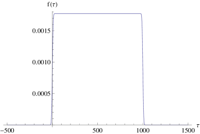
Figure 1: The plot illustrates the form of the external force defined by an analytical function of the proper time along the whole real axis. Note that the force can be seen as an infinitely differentiable regularization of an exact square pulse showing the discontinuities at the times $\tau=0\,\,$s and $\tau=1000\,\,$s .

Dirac , in order to illustrate the appearance of runaway solutions in the ALD equations. For the values of the parameters giving a force in the form  square pulse, it will be shown that the solution predicted by the effective Newton equations does not show the runaway, nor the pre-accelerated behavior, exhibited by the solutions derived by Dirac. However, it will be also numerically checked that these solutions also satisfy the ALD equations.

The explicit form of the ”regularized” pulse defining the force in the rest frame of the particle will be

$$f(\tau,t_{o},T) =f_{o}\int_{0}^{T}ds\exp(-\frac{(\tau-s)^{2}}{f_{1}^{2}t_{o}^{2}})$$

$$=5\sqrt{\pi}t_{o}\text{ }f_{o}(Erf\text{ }(\frac{(T-\tau)}{f_{1}\text{ }t_{o}})+Erf\text{ }(\frac{\tau}{f_{1}\text{ }t_{o}})),$$ (34)

$$f_{o} =\frac{1}{10000},\text{ \ \ }f_{1}=10.$$ (35)

where $Erf$ is the Error Function.  The defined force is depicted in figure 1 for the chosen values of  $t_{o}=1$ cm and $T$ $=$1000 cm. note that we are expressing the time in normal units.   Let us no consider the series defining the effective force $f_{e}(\tau),$  which is associated to the external force $f(\tau):$

$$f_{e}(\tau)=S_{\infty}^{\text{\ }}(\tau)=\sum_{m=0}^{\infty}\frac{d^{m}}{d\tau^{m}}f(\tau)\text{ }(\frac{\kappa}{m})^{m}.$$ (36)

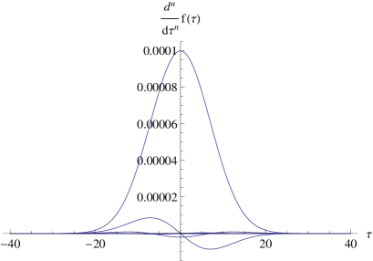
Figure 2: The figure shows the plots of the proper time derivatives up to the order ten, of the force function associated to the defined analytic regularization of the square pulse. The plot was done in a range of the origin of coordinates in which the derivatives show the higher values, since the pulse is transiting to attain its constant non vanishing value. As it can be observed, all these derivatives are bounded functions of the proper time. Even more, the bounds for the derivatives decrease with their order. This behavior is maintained up to high values of the derivatives of order 50, where the numerical errors started distorting the numerical results.

But, given $\frac{\kappa}{m}<1,$ which is extremely well satisfied by the case of the electromagnetic ALD equation, the series defining the effective force will converge just by only requiring that the time derivatives of arbitrary order are uniformly bounded for all time values. The satisfaction of this condition for the specific form to be considered for the force, after fixing $t_{o}=1$ cm and $T$ $=1000$ cm, is evidenced in figure 2. It shows the plots of the times derivatives of orders $n=1,2,3,...,9,10.$ It can be observed that all the depicted times derivatives are bounded, and moreover the bound decreases when the order of the derivatives increases. This behavior is maintained for higher orders, up to values in which the numerical precision becomes degraded in our evaluation.

However, before assuming the form of the force in (35) by fixing the values of $t_{o}$ and $T$ ,  it can be argued that the effective pulse like forces are also well defined for extremely short ”rising” times $t_{o}$ and arbitrarily large time lapses $T$ of the pulses. This property can be argued after performing the changes of variables

$$\tau=t_{o}\text{ }x,\text{ \ }s=t_{o}\text{ }y,$$ (37)

which allows to express the force $f$ in the form

$$f(\tau,t_{o},T) =f^{\ast}(x,t_{o},\frac{T}{t_{o}})$$

$$=f_{o}t_{o}\int_{0}^{\frac{T}{t_{o}}}dy\exp(-(\frac{x-y}{f_{1}})^{2})$$

$$=5\sqrt{\pi}t_{o}\text{ }f_{o}(Erf(\frac{(\frac{T}{t_{o}}-x)}{f_{1}\text{ }})+Erf(\frac{x}{f_{1}\text{ }})).$$ (38)

But, the implemented change of variables, allows to write for the effective force series

$$f_{e}(\tau) =\sum_{m=0}^{\infty}\frac{d^{m}}{dt^{m}}f(t,t_{o},T)(\frac{\kappa}{m})^{m},$$

$$=\sum_{m=0}^{\infty}\frac{d^{m}}{dx^{m}}f^{\ast}(x,t_{o},\frac{T}{t_{o}})(\frac{\kappa}{m}\frac{1}{t_{o}})^{m}.$$ (39)

The last line of this relation, again indicates that with the ”rising” time being so short as to merely satisfying

$$t_{o}>\frac{\kappa}{m},$$ (40)

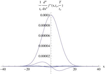
Figure 3: The behavior of the derivatives respect to the variable $x$ of the auxiliary functions $f^{\ast}$ . The plots show derivatives up to the order ten of the function $f^{\ast}$ being associated to the defined analytic regularization of the square pulse. The graphic corresponds to a range of the origin of coordinates in which the derivatives show the higher values. Again all these derivatives are bounded functions of the coordinate $x$.

the effective force as a function of the time (or equivalently the variable $x$) becomes well defined if the arbitrary derivatives over $x$ of the function $\ f^{\ast}(x,t_{o},\frac{T}{t_{o}})$ are uniformly bounded for all the considered values of the variable $x$. But, figure 3 illustrates that the values of these derivatives as functions of $\ x$  up to order ten, are bounded at all the values of the $x$ variable. This behavior is valid up to high orders for which the numerical precision of the evaluations start to become degraded. Therefore, the results indicate that the regularized constant force pulses, constructed in the described analytic way, well define effective forces for very fast pulses, which can rise so rapidly as few times the ALD time constant of nearly 10^-24 seconds in the electromagnetic case.

IV.2 Solutions of the Newton equations for the regularized pulsed force

The equations for the coordinates as functions of the proper time for the pulsed force with the times parameters $t_{o}=1$ cm and $T$ $=1000$ cm will be now numerically solved. With the use of their definition (21) these equations can be written in the form

$$a^{\mu}(\tau) =\frac{1}{m}\mathcal{F}^{\mu}\mathcal{(\tau)},$$ (41)

$$\mathcal{F}^{\mu}\mathcal{(\tau)} =(\gamma\overrightarrow{v}.\overrightarrow{f_{e}},\text{ }\overrightarrow{f_{e}}+(\gamma-1)\frac{\overrightarrow{v}.\overrightarrow{f_{e}}}{v^{2}}\overrightarrow{v}),$$ (42)

$$\overrightarrow{f_{e}} =\sum_{m=0}^{\infty}\frac{d^{m}}{dt^{m}}f(\tau,t_{o},T)(\frac{\kappa}{m})^{m}.$$ (43)

In this 2D case we have the definitions

$$u^{\mu}(\tau) \equiv(\gamma,\gamma\overrightarrow{v}),$$ (44)

$$a^{\mu}(\tau) \equiv(\frac{d}{d\tau}\gamma,\frac{d}{d\tau}(\gamma\overrightarrow{v})).$$ (45)

The  following two Newton equations can be explicitly written in the form

$$\frac{d}{d\tau}u(\tau) =\frac{1}{m}\gamma\text{ }f_{e}(\mathcal{\tau)},$$ (46)

$$\frac{d}{d\tau}u^{0}(\tau) =\frac{1}{m}\gamma\text{ }f_{e}(\mathcal{\tau)}v(\tau),$$ (47)

$$\gamma(\overrightarrow{v}) =\sqrt{1-v^{2}},\text{ \ \ }v^{2}=\overrightarrow{v}.\overrightarrow{v}.$$ (48)

But employing the definitions of the spatial velocity $\overrightarrow{v}$, 4-velocity $u^{\mu}$ and the effective forces $f_{e}$

$$\overrightarrow{v}(\tau) =\frac{d}{dt}\overrightarrow{x}=\frac{d}{\gamma d\tau}\overrightarrow{x}(\tau),$$ (49)

$$u^{\mu} =\frac{d}{d\tau}x^{\mu}(\tau),$$ (50)

$$\overrightarrow{f_{e}} =\sum_{m=0}^{\infty}\frac{d^{m}}{d\tau^{m}}f(\tau,t_{o},T)(\frac{\kappa}{m})^{m},$$ (51)

the equations for the position and the time describing the trajectories $(t(\tau),$ $x(\tau))$ which solve the Newton equations become

$$\frac{d^{2}}{d\tau^{2}}x(\tau) =\frac{1}{m}\frac{d}{d\tau}t(\tau)\text{ }\sum_{m=0}^{\infty}\frac{d^{m}}{d\tau^{m}}f(\tau,t_{o},T)(\frac{\kappa}{m})^{m},$$

$$\frac{d^{2}}{d\tau^{2}}t(\tau) =\frac{1}{m}\text{ }\frac{d}{d\tau}x(\tau)\sum_{m=0}^{\infty}\frac{d^{m}}{d\tau^{m}}f(\tau,t_{o},T)\text{ }(\frac{\kappa}{m})^{m}.$$ (52)

These equations are now solved for the particular values of the parameters

$$t_{o} =1\text{ \ \ cm,}$$ (53)

$$T =1000\text{ \ cm.}$$ (54)

The constant $\frac{\kappa}{m}$ will be set to a value being in fact very much higher than the one associated to the electron motion, which is nearly 10${}^{-24}c$ cm. The chosen specific value $\frac{\kappa}{m}=0.8$ cm will help to avoid extremely small higher orders contributions in powers of $\frac{\kappa}{m}$, in the numerical solution of these equations. It can be noticed that very much larger values of $\frac{\kappa}{m}$ with respect to the one associated with the electron, are also of  physical interest, by example when considering the radiation of small moving objects in the air. The solutions of the equations were considered for the following initial conditions

$$x(-50) =0,$$ (55)

$$\frac{d}{d\tau}x(-50) =0.2.$$ (56)

That is, at a proper time value of $-50$ cm , the particle is situated at the origin of coordinates with a velocity given the proper time derivative of its coordinates (the spatial component of the four-velocity) equal to $0.2$.   It can be noted that this problem is similar to the one considered by Dirac to illustrate the appearance of pre-acceleration in the solutions of the ALD equations Dirac . The main difference between the two situations  is that here the pulse is not rigorously squared  with discontinuous step like transitions, but defined by an analytic function along the whole time axis.

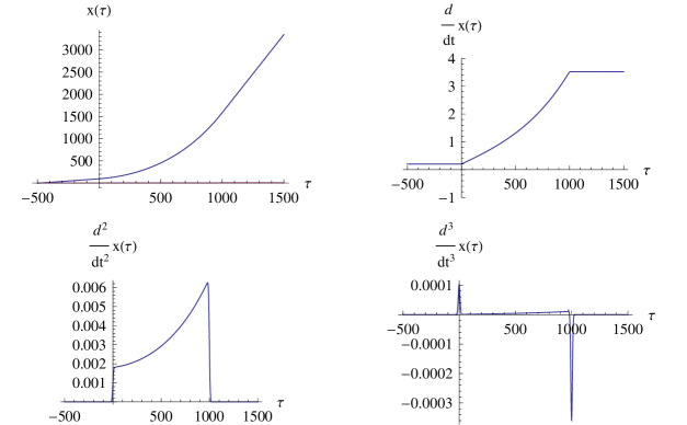
Figure 4: The top left figure depicts the proper time evolution of the coordinates of the particle upon which the force is acting. The top right one, then shows the velocity of the particle in the same proper time interval. It is clear that the motion tends to be uniform, outside of the interval $(0,1000)$. The bottom left figure shows the behavior of the acceleration which tends to vanishes outside the times in which the pulse gets appreciable values. The last graph presents the dependence of the time derivative of the acceleration. This quantity tends to be peaked around the instants at which the pulse drastically changes its value.

The form of this pulse was shown in figure 1. The high value of the ratio $\frac{T}{t_{o}}$ gives to this function the approximate pulse like appearance. The set of plots in figure 4 shows in first place, the proper time evolution of the coordinate of the particle, indicating that the motion is nearly free before the time interval of the pulse, for becoming accelerated for the times in which the force is nearly constant. When the times is large and outside the region in which the force is constant, the solutions becomes again a uniform motion as illustrated by the vanishing of the acceleration in this zone. Note that the solution of the Newton equations do not exhibit the pre-acceleration effect, nor the runaway motions after the pulse is passed, as it was the case in the Dirac solution of the ALD equations Dirac . This is not a strange result given that the effective force tends to vanish outside the pulse interval.  However, this example allows to numerically check that the obtained solution also satisfies the ALD equations. This is clearly illustrated in figure 5. It shows the plot of the following function, which vanishes when the ALD equations are satisfied

$$E_{ALD}(\tau)=ma(\tau)-f(\tau)-\varkappa\text{ }(\frac{d}{d\tau}a(\tau)+a^{\nu}(\tau)a_{\nu}(\tau)u(\tau)),$$ (57)

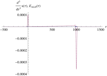
Figure 5: The figure shows two plots in common: the value of the derivative of the acceleration, which is the smaller term among the various contributions to the ALD equations, and the function $E_{ALD}$ which vanishing implies the satisfaction of the spatial ALD equation. The fact that the values of the function $E_{ALD}$ can not be noticed in the plot, checks the very approximate satisfaction of the spatial ALD equation

in common with the plot of the time derivative of the acceleration term of the ALD equations, which is the term of the equations showing, in general, the smaller values along the times axis. As it can be noticed, the values of the function $\ E_{ALD}(\tau)$ can not be noticed in comparison with the values of the third derivative term. This indicates that the ALD equations are satisfied within the precision of the numerical approximation of the solution, confirming the general derivation presented before. Therefore an interesting conclusion arises: the obtained solution of the effective Newton equation, at the same time that also satisfies the ALD equation,  avoids the appearance of the pre-acceleration or runaways effects.

This example of an analytically regularized pulse, leads to an idea about how justify a modification of the ALD equations for the case of non analytically defined forces, presented in reference cabojorge . This point will discussed in next sections.

V  Modified ALD equations for forces with sudden changes

We will now assume that the existence of a sequence of forces $f_{k}^{\mu}(\tau),$ $\ k=1,2,....\infty$ in all the proper time axis, which also show, for each $k$, convergent values of the series defining their effective forces $\ f_{e,k}^{\mu}(\tau),$ $\ k=1,2,....\infty$.   A first general purpose of this section will be to argue that, assumed that the sequence $f_{k}^{\mu}(\tau)$ converges to a piecewise continuous limiting force $f^{\mu}(\tau)$, the sequence of solutions of the corresponding effective Newton equations ALD equations will tend to satisfy a set of modified ALD equations, which form will be also determined. It will follow that these equations just generalize the ones which were proposed in reference cabojorge .  In that work, these equations were simply advanced under the basis of an idea: when a force acting over a radiating classical electron is instantly removed, the Lienard –Wiechert solution for the electromagnetic field surrounding the electron within a sufficiently close neighborhood of its position, should be instantly defined by a Lorentz boost transformed Coulomb field. But such fields, are known to exert a vanishing four-force over the electron. This simple observation strongly suggests that the mechanical equations driving the electron motion, should be able to reproduce this effect: that is, to instantaneously lead the acceleration of the particle to vanish, when a force is removed in a extremely rapid way.  The here found equations of motion implement this property.

Let us firstly consider that the proper time axis is subdivided in a denumerable set of contiguous  intervals by the specific sequence of increasing values of times

$$(\tau_{o},\tau_{o}^{(k)\ast},\tau_{1},\tau_{1}^{(k)\ast},\tau_{2},\tau_{2}^{(k)\ast},...\tau_{n},\tau_{n}^{(k)\ast},.....).$$ (58)

The general intervals ($\tau_{n},\tau_{n}^{(k)\ast})$ for arbitrary $n$ values will be called as the ”transition” intervals, in which the arbitrary time derivatives for the forces of the sequence of $\ f_{k}^{\mu}(\tau)$ for all $k$ values will be assumed as well defined, by also determining bounded values for the effective forces $f_{e,k}^{\mu}(\tau)$ for all values of $k.$  In the limit $k\rightarrow\infty$ we will assume that all the times $\tau_{n}$ not showing the superindex $k$,  will remain constant, and the other instant will have limits $\tau_{n}^{(k)\ast}\rightarrow\tau_{n}.$  In the limit $k\rightarrow\infty$ the sequence of forces will be assumed to possibly approach a piecewise discontinuous limiting force at the points $\tau_{n}$ at all $n$ values.

On the opposite way, within all the intervals $(\tau_{n}^{(k)\ast},\tau_{n+1})$ the sequence of force functions will be assumed to tend to an infinitely smooth function of the proper time, by also leading to well defined effective forces. In particular if the force functions are given by polynomial functions of the proper time with maximal order $N_{max}$, the series defining the effective forces, having a finite number of terms, will always well define effective forces.

Due to the assumption about the existence of the sequence of effective forces along all the whole time axis for all finite $k$ values, the effective Newton equations will be properly defined for all $k$ , and can be solved by simply integrating over the proper time. We assume that the sequence of the effective forces $f_{e,k}^{\mu}(\tau)$ will also tend to be piecewise continuous and bounded at all the time axis. Then, this condition will imply that the time integrals of the forces within all the transition intervals $(\tau_{n},\tau_{n}^{(k)\ast})$ should vanish when these intervals shrink in the limit $k\rightarrow\infty.$   Therefore, since integrals of this sort will define the discontinuity in the four-velocities in the limit $k\rightarrow\infty,$ it follows that the four-velocities should be continuous in the $k\rightarrow\infty$ limit.

V.1 The modified ALD equations

Consider now the sequence of the solutions of the of the effective Newton equations $x^{(k)\mu}(\tau)$ for all values of $k$. From the previous discussion, it is clear that for each $k$ value, the 4-velocities as functions of the time will not tend to develop discontinuities across the transition intervals when they reduce their sizes in the limit $k\rightarrow\infty.$  This follows, because the effective forces are assumed to exist and to be also bounded. Thus, the impulses  of these forces during the shrinking  transition intervals should tend to zero. Therefore, we will have that the sequence of solutions tend to be piecewise smooth trajectory $x^{(k)\mu}(\tau)$ showing also a continuous velocity at the transition points in the $k\rightarrow\infty$ limit.

Strictly inside all the intervals ($\tau_{n}^{(k)\ast},$ $\tau_{n+1})$ the solutions $\ x^{(k)\mu}(\tau)$ can be constructed as satisfying the $k\rightarrow\infty$ limit of the Newton equation, since the limiting $k\rightarrow\infty$ values of the forces and the effective forces within these intervals are assumed to be smooth and also bounded. Then, in these zones they will also satisfy the ALD equation  Therefore, within each of these intervals the limiting $k\rightarrow\infty$ trajectory $x^{\mu}(\tau)$ should satisfy the effective Newton equations

$$ma^{\mu}(\tau) =\mathcal{F}^{(n)\mu}\mathcal{(}\tau\mathcal{)}$$

$$\equiv(\gamma(v)\overrightarrow{v}(\tau).\overrightarrow{f_{e}}^{(n)}(\tau),\overrightarrow{f_{e}}^{(n)}(\tau)+(\gamma-1)\frac{\overrightarrow{v}\text{ }\overrightarrow{f_{e}}^{(n)}(\tau)}{v^{2}}\overrightarrow{v}),$$ (59)

in which the effective forces $\ \ \overrightarrow{f_{e}}^{(n)}$ are defined by

$$\overrightarrow{f_{e}}^{(n)}=\sum_{m=0}^{\infty}\frac{d^{m}}{dt^{m}}\overrightarrow{f}^{(n)}(\tau)(\frac{\kappa}{m})^{m},$$ (60)

with $\overrightarrow{f}^{(n)}(\tau)$ being the limit $k\rightarrow\infty$ of the sequence of forces $f_{k}^{\mu}(\tau)$ for the time taken within the interval ($\tau_{n},\tau_{n+1}).$ At this point, as noted in the introduction, we will restrict the discussion in this section to collinear motions. The generalization to arbitrary motions seems to be feasible, and it will be considered elsewhere.

However, due to the assumed developing of step like discontinuities of the force values after the limit $k\rightarrow\infty,$ at the transition points $\tau_{n},$ we can have for the effective four-force possibly different values at the left $\tau_{n}^{-}$ and right $\tau_{n}^{+}$ of the transition instants, with values

$$\mathcal{F}^{\mu}\mathcal{(}t_{n}^{-}\mathcal{)} \equiv\left.(\gamma(v)\overrightarrow{v}(\tau).\overrightarrow{f_{e}}^{(n-1)}(\tau),\overrightarrow{f_{e}}^{(n-1)}(\tau)+(\gamma-1)\frac{\overrightarrow{v}\text{ }\overrightarrow{f_{n}}^{(n-1)}(\tau)}{v^{2}}\overrightarrow{v})\right|_{\tau=\tau_{n}^{-}},$$ (61)

$$\mathcal{F}^{\mathcal{\mu}}\mathcal{(}t_{n}^{+}\mathcal{)} \equiv\left.(\gamma(v)\overrightarrow{v}(\tau).\overrightarrow{f_{e}}^{(n)}(\tau),\overrightarrow{f_{e}}^{(n)}(\tau)+(\gamma-1)\frac{\overrightarrow{v}\text{ }\overrightarrow{f_{n}}^{(n)}(\tau)}{v^{2}}\overrightarrow{v})\right|_{\tau=\tau_{n}^{+}},$$ (62)

where, as noted before the coordinates and velocities are continuous at both sides of the  transition point $\tau_{n}.$ We will also define the force functions inside each of the intervals $(t_{n},t_{n+1})$ as $\mathcal{F}^{(n)\mu}\mathcal{(}\tau\mathcal{)}=\mathcal{F}^{\mathcal{\mu}}\mathcal{(}\tau\mathcal{)}$ for $\tau$ $\epsilon$ $(\tau_{n},\tau_{n+1}).$ Thus $\mathcal{F}^{\mu}\mathcal{(}\tau_{n}^{-}\mathcal{)}=\mathcal{F}^{(n)\mu}\mathcal{(}\tau_{n}\mathcal{)}.$ Since these two limiting forces are equal to the mass $m$ times de accelerations at any instant,  this relation says that the accelerations can be discontinuous at those instants.  This property defines a clear deviation from the case of the solutions showing pre-acceleration or runaway behavior, which are assumed to have continuous accelerations  Dirac .

Then, let us now argue that the effective equations (59)  with the two boundary conditions (61),(62) are equivalent to the set of modified ALD equations

$$ma^{\mu}(\tau)-f^{\mu}(\tau) =\varkappa\text{ }(\frac{d}{d\tau}a^{\mu}(\tau)+a^{\nu}(\tau)a_{\nu}(\tau)u^{\mu}(\tau))+$$

$$+\frac{\varkappa}{m}\sum_{n=0}^{\infty}(\mathcal{F}^{\mu}\mathcal{(}t_{n}^{-}\mathcal{)}\delta^{(D,-)}(\tau-\tau_{n})-\mathcal{F}^{\mu}(\tau_{n}^{+})\delta^{(D,+)}(\tau-\tau_{n}),$$ (63)

where  the Dirac Delta function, let say $\delta^{(D,-)}(\tau)$   is defined as linear functionals determined by a sequence of functions of time $\delta_{k}^{(D,-)}$($\tau),k=1,2,3,...,$ all having time integrals equal to the unit for any $k$ value. Their supports for each $k$ is defined by intervals $(-\epsilon_{k},0),$ with positive $\epsilon_{k}$, which tend to vanish in the limit $k\rightarrow\infty$. The linear functional acting over a possibly piecewise continuous function $g(\tau)$ is then defined as the integral

$$\lim_{\tau\rightarrow 0^{-}}(g(\tau))=\lim_{k\rightarrow\infty}\int d\tau\text{ }\delta_{k}^{(D,-)}(\tau)g(\tau).$$ (64)

Therefore, if the function $g$ has a discontinuity of the step function type, the integral of the function $\delta^{(D,-)}(\tau-\tau_{n})$ will give the value of the limit of $g$ at the left of the point $\tau_{n}.$ The right Dirac Delta $\delta^{(D,+)}(\tau)$ is defined in a similar way, but with support of the form  $(0$, $\epsilon_{k})$ with all $\epsilon_{k}$ again positive.

Now let us consider the acceleration $a^{\mu}(\tau)$ defined by the effective force in a sufficiently small open neighborhood $B_{n}$ of each instant $t_{n}.$ The expression for it can be written in the form

$$a^{\mu}(\tau)=\frac{\mathcal{F}^{(n-1)\mu}\mathcal{(}\tau\mathcal{)}}{m}\Theta^{(-)}\mathcal{(}\tau_{n.}-\tau)\text{+}\frac{\mathcal{F}^{(n)\mu}\mathcal{(}\tau\mathcal{)}}{m}\Theta^{(+)}\mathcal{(}\tau-\tau_{n.}),_{.}$$ (65)

where the special Heaviside like functions are defined as $\Theta^{(\pm)}\mathcal{(}\tau)=\int_{-\infty}^{\tau}ds$ $\delta^{(D,\pm)}(s).$Therefore, let us search for the equation satisfied by this expression for the acceleration.  The derivative of the acceleration within the neighborhood $B_{n}$ takes the form

$$\frac{d}{d\tau}a^{\mu}(\tau) ={\Large(}\frac{d}{d\tau}(\frac{\mathcal{F}^{(n-1)\mu}\mathcal{(}\tau\mathcal{)}}{m})\Theta^{(-)}\mathcal{(}\tau_{n.}-\tau)\text{+}\frac{d}{d\tau}(\frac{\mathcal{F}^{(n)\mu}\mathcal{(}\tau\mathcal{)}}{m})\Theta^{(+)}(\tau-\tau_{n.})$$

$$+\frac{\mathcal{F}^{(n-1)\mu}\mathcal{(}\tau\mathcal{)}}{m}\frac{d}{d\tau}\Theta^{(-)}\mathcal{(}\tau_{n.}-\tau)\text{+}\frac{\mathcal{F}^{(n)\mu}\mathcal{(}\tau\mathcal{)}}{m}\frac{d}{d\tau}\Theta^{(+)}(\tau-\tau_{n.}){\Large)}$$

$$={\Large(}\frac{d}{d\tau}(\frac{\mathcal{F}^{(n-1)\mu}\mathcal{(}\tau\mathcal{)}}{m})\Theta^{(-)}\mathcal{(}\tau_{n.}-\tau)\text{+}\frac{d}{d\tau}\frac{\mathcal{F}^{(n)\mu}\mathcal{(}\tau\mathcal{)}}{m}\Theta^{(+)}(\tau-\tau_{n.})+$$

$$-\frac{\mathcal{F}^{(n-1)\mu}\mathcal{(}\tau\mathcal{)}}{m}\delta^{(D,-)}(\tau-\tau_{n})\text{+}\frac{\mathcal{F}^{(n)\mu}\mathcal{(}\tau\mathcal{)}}{m}\delta^{(D,+)}(\tau-\tau_{n}){\Large)}.$$ (66)

Henceforth, after substituting this expression in (63), and considering that the ALD equations are satisfied at the interior points of all the intervals $(\tau_{n},\tau_{n+1}),$ it follows

$${\LARGE(}{\large(}ma^{\mu}(\tau)-f^{\mu(n-1)}(\tau)-\varkappa\text{ }(\frac{d}{d\tau}a^{\mu}(\tau)+a^{\nu}(\tau)a_{\nu}(\tau)u^{\mu}(\tau)){\large)}\mathcal{\Theta}^{(-)}\mathcal{(}\tau_{n.}-\tau)+$$

$${\large(}ma^{\mu}(\tau)-f^{\mu(n)}(\tau)-\varkappa\text{ }(\frac{d}{d\tau}a^{\mu}(\tau)+a^{\nu}(\tau)a_{\nu}(\tau)u^{\mu}(\tau)){\large)}\mathcal{\Theta}^{(+)}\mathcal{(}\tau-\tau_{n.})$$

$$-\frac{\varkappa\mathcal{F}^{(n-1)\mu}\mathcal{(}\tau\mathcal{)}}{m}\delta^{(D,-)}(\tau-\tau_{n})+\frac{\varkappa\mathcal{F}^{(n)\mu}\mathcal{(}\tau\mathcal{)}}{m}\delta^{(D,+)}(\tau-\tau_{n}).$$

$$+\frac{\varkappa}{m}(\mathcal{F}^{\mu}\mathcal{(}\tau_{n}^{-}\mathcal{)}\delta^{(D,-)}(\tau-\tau_{n})-\mathcal{F}^{\mu}(\tau_{n}^{+})\delta^{(D,+)}(\tau-\tau_{n}){\LARGE)}=0.$$ (67)

Thus, all the terms in the above equations add to zero around each transition time $t_{n}$. The first two lines line vanish because the trajectories solving the Newton equations within each of the intervals $(\tau_{n},\tau_{n+1})$ also satisfy the ALD equations within each neighborhood $B_{n}$except at the point $t_{n}$. The last two terms also cancels between themselves since the Delta functions allow to evaluate the argument of the functions multiplying them at their support point. Therefore, after considering that the modifying terms of the ALD equations vanish outside all the vicinities $B_{n},$   it follows that the limiting solution along the whole axis satisfies the modified ALD equations

$$ma^{\mu}(\tau)-f^{\mu}(\tau) =\varkappa\text{ }(\frac{d}{d\tau}a^{\mu}(\tau)+a^{\nu}(\tau)a_{\nu}(\tau)u^{\mu}(\tau))+$$

$$+\varkappa\sum_{n=0}^{\infty}(a^{\mu}(\tau_{n}^{-})\delta^{(D,-)}(\tau-\tau_{n})-a^{\mu}(\tau_{n}^{+})\delta^{(D,+)}(\tau-\tau_{n}).$$ (68)

V.2 The solution for the constant force pulse

Let us consider now the solution of the modified ALD equations for the case of a exact squared pulse of the similar form as the before considered analytic one. The same initial conditions for the position and velocities will be fixed

$$x(-50) =0,$$ (69)

$$\frac{d}{d\tau}x(-50) =0.2.$$ (70)

The Newton equations in the interior points of any of the three intervals in which the time axis is decomposed by the two instants $\tau_{o}=0$ and $\tau_{1}=T,$ have basically the same form as the equation (52)

$$\frac{ds^{2}}{d\tau^{2}}x(\tau) =\frac{1}{m}\frac{d}{d\tau}t(\tau)\text{ }f_{P}(\tau,T),$$

$$\frac{d^{2}}{d\tau^{2}}t(\tau) =\frac{1}{m}\text{ }\frac{d}{d\tau}x(\tau)f_{P}(\tau,T),$$ (71)

where the force now defining the exact pulse of constant amplitude is given by the formula

$$f_{P}(\tau,T)=f^{p\text{ }}\Theta(\tau)\text{ }\Theta(T-\tau),$$ (72)

in which $\Theta(\tau)$ is the Heaviside function. The width of the pulse was chosen as given by the same parameter $T$ defining the width of the analytically regularized pulse in past sections. The constant amplitude of the pulse $f^{p\text{ }}$ will be approximately coinciding with the  height of the  regularized pulse, by selecting its magnitude as

$$f^{p\text{ }}=f(\frac{T}{2},t_{o},T).$$ (73)

That is, by the height of the pulse at a time equal to half of its approximate width $T$ . The parameters for the numerical evaluation will also coincide with values selected before  $t_{o}=1$ and $\ T=1000.$

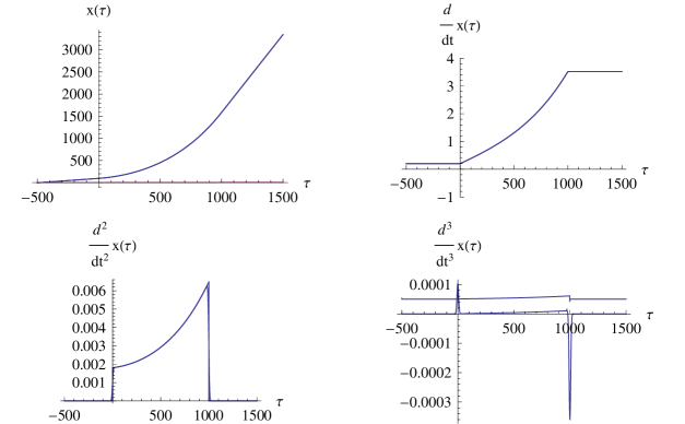
Figure 6: The array of figures show in each graphic two plots, one associated to the analytic pulse of force and the other relate with the exact square pulse solving the modified ALD equations. The top left figure shows the coordinates of both solutions. Note the close coincidence of the coordinates. The top right curves for the velocities also illustrates the similarity between the solutions for this quantity. The bottom left plot present the results for the accelerations for the two solutions. The non constant behavior of the acceleration shows that the motion is relativistic. Finally the bottom right plot compares the time derivatives of the acceleration for both solutions. For better evidencing the difference, the quantity associated to the exactly square pulse is shifted in a positive constant along the vertical axis. It can be noted that in the internals points of the interval $(0,1000)$ the two evaluations tend to coincide. However, in the points close to the boundaries of this interval, the derivative of the acceleration associated to the analytic pulse develops peaked values. These peaked values gives account of the developing of the Dirac functions entering the modified ALD equations. The analytic solution, as obeying the exact ALD along the whole axis should generate these Dirac functions, in order to imply the modified equations in the limit.

The solution of the equations (71) for the time dependence of the coordinate, velocity, acceleration and its time derivative,  are jointly plotted in figure 6, for both pulses: the one of exactly constant amplitude and the analytically regularized one.  The plots evidence that these quantities are closely similar for both forces. A small difference starts to be noticed in the curve for the velocities. It shows that only in the close neighborhood of the transition points, in which the forces suddenly change, the rapid but smooth transition of the velocity for the  regularized pulse can be observed. Further, the plot of the derivative of the acceleration is also presenting a difference.  For making the comparison clearer, the plot associated to the derivative of the acceleration for the pulse of exact constant amplitude, is slightly shifted along the vertical axis away the zero values.  This permits to note that the magnitude of the derivative of the acceleration at the interior points of the interval $(0,T)$ closely coincide for both solutions. However, near the transition points, the regularized pulse presents a peaked behavior.  This is a numerical confirmation for the validity of the modified equations, since these peaked dependence are necessary for reproducing the Dirac’s delta functions entering these modified equations, in the limit when the regularized pulse tends to becomes the exactly constant one. That is, when the regularized pulse is gradually made to be even more similar to the constant pulse, it can be expected that the ”spikes” appearing at the transition points for the derivatives of the acceleration, are associated to regularizations of the Dirac’s distributions. The enhancing of the peaks when the regularized pulse tends to be closer to the exact constant ones is illustrated in figure 7. It shows the derivative of the acceleration for two solutions with almost all the parameters identical to the ones considered before, but differing only in the value determining the pulse rise time $t_{o}$.

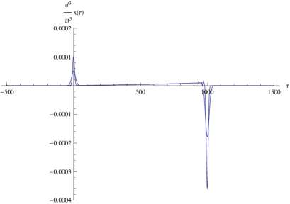
Figure 7: The superposed plot corresponds to two analytic pulsed forces of nearly equal height and width, but one having a rising time double than the other. One curve is related with the higher left and right peaks, and the other is associated with lower ones at both sides. The curve showing the higher peaks corresponds to the pulse with shorter rising time, which illustrates how the Dirac’ Delta functions appearing in the modified ALD equations are gradually generated as the pulse approaches the exactly squared form.

The values selected for this parameters were $t_{o}=1$ cm and $t_{o}=2$ cm.  That is, the pulse with $t_{o}=1$ will have a rising time two times smaller than the one with $t_{o}=2$ m. In the picture, there is a curve which shows the smaller peaks at the right and left of the figure, and the other one presents the higher peaks at both sides.  The curve with the larger values is associated to the pulse $t_{o}=1$ and the curve with smaller values is related with the slower rising pulse. Thus, it is clear that when the analytic pulse tends to approach the exactly constant one, the solution tends to show time derivatives with the appearance of  regularizations of the Dirac’s Delta functions, as the it should be, if the modified ALD equations are implied by the limit of the exact ALD equations.

The absence of the peaks in the solution linked with the square pulse is associate with the fact that the equations were solved at the interior points, and the boundary conditions are automatically satisfied across the two transition points, by the solutions of the Newton equations in the three intervals. These boundary conditions were argued before to be equivalent to the presence of Dirac Delta functions with supports in the transition points.

Summary

The work presents a second order Newton like equations of motion for a radiating particle. It was argued that the trajectories obeying the equation exactly satisfy the Abraham-Lorentz-Dirac (ALD) equations. Forces which only depend on the proper time were considered by now. A condition for these properties to occurs in a given time interval is derived: it is sufficient that the force becomes infinitely smooth and also that a particular series defined by the infinite sequence of its time derivatives converges to a bounded function. This series defines in a local way the effective force determining the Newton effective equation. The existing solutions of such effective equations can not show the runaways or pre-acceleration phenomena. The Newton equations were numerically solved for a pulsed like force given by an analytic function on the whole proper time axis. The satisfaction of the ALD equations by the obtained solution is numerically checked. In addition, for the case of the collinear motions, it was derived a set of modified ALD equations for almost infinitely smooth forces, which however, show step like discontinuities. The form of these equations supported the statement argued in a former work, about that the Lienard-Wiechert field surrounding a radiating particle should determine that the effective force on the particle instantaneously vanishes, when the external force is suddenly removed. The modified ALD equations argued in the former study are here derived in a more general form, in which a suddenly applied external force is also instantly creating an effective non vanishing acceleration. The work is expected to be extended in some directions. By example, one issue which seems of interest to define is whether the class of external forces which also show well defined effective forces, constitutes a dense subset (within an appropriate norm) at least within the set of forces defined by continuous proper time functions. This property could help to understand, whether the ALD equations, for any continuous time dependent force, could always exhibit a solution, which is also approximately solving second order Newton equations, and then not showing pre-accelerated or runaway behavior.

References

- (1) H. A. Lorentz, The theory of electrons, Leipzig: Teubner, 1909 (2nd edition, 1916).
- (2) M. Abraham, Theorie der Elektrizitat, V. 2: Elektromagnetische, Theorie der Strahlung, Leipzig: Teubner, 1905.
- (3) H. Poincare, On the dynamics of the electron, Rendiconti del Circulo Matematico de Palermo 21, 129-176, 1906.
- (4) G. A. Schott, Electromagnetic radiation, Cambridge University Press, 1912.
- (5) P. A. M. Dirac, Proc. Roy. Soc. A 167, 148, 1938.
- (6) C. Teitelboim, D. Villarroel and Ch. G. van Weerth, Rev. Nuov. Cim. 3, 1, 1980.
- (7) F. Rohrlich, Classical charged particles, Redwood City, CA: Addison-Wesley, 1990.
- (8) A. Yaghjian, Relativistic dynamics of a charged particle, Lecture notes in Physcs, m11, Springer Verlag, New York, Berlin, Heidelberg, 1992.
- (9) G. W. Ford and R. F. O’Connell, Phys. Letts. A157, 17, 1991.
- (10) H. Spohn, Dynamics of charged particles and their radiation field, Cambridge University Press, Cambridge, 2004.
- (11) C. K. Raju and S. Raju, Radiative damping and functional differential equations, arXiv.0802.3390v2 (2008)
- (12) L. D. Landau, and E. M. Lifshitz, The classical theory of fields, Addison-Wesley, London 1959.
- (13) E. M. Purcell, Electricidade e Magnetismo, Curso de Fisica de Berkeley, V. 2, Edgar Blucher, Sao Paolo 1973.
- (14) D. Vogt and P. S. Letelier, Gen. Rel. Grav. 35, 2261, 2003.
- (15) A. Cabo Montes de Oca and J. Castiñeiras, On radiation reaction and the Abraham-Lorentz-Dirac equation, arXiv:1304.2203 [gr-qc], 2013.