Packing hard spheres with short-range attraction in infinite
dimension:
Phase structure and algorithmic implications
Abstract
We study, via the replica method of disordered systems, the packing problem of hard-spheres with a square-well attractive potential when the space dimensionality, , becomes infinitely large. The phase diagram of the system exhibits reentrancy of the liquid-glass transition line, two distinct glass states and a glass-to-glass transition, much similar to what has been previously obtained by Mode-Coupling Theory, numerical simulations and experiments. The presence of the phase reentrance implies that for a suitable choice of the intensity and attraction range, high-density sphere packings more compact than the one corresponding to pure hard-spheres can be constructed in polynomial time in the number of particles (at fixed, large ) for packing fractions . Although our derivation is not a formal mathematical proof, we believe it meets the standards of rigor of theoretical physics, and at this level of rigor it provides a small improvement of the lower bound on the sphere packing problem.
1 Introduction
Packing problems [1] are ubiquitous in science and engineering and arise in a variety of contexts ranging from biology (e.g. in the crowded cellular environment where physiological processes conspire significantly with excluded-volume effects [2]) to communication technology (e.g. in connection with the design of error correcting codes for signal transmission over noisy channels [3]). From a mathematic [4, 5] and algorithmic [1, 6, 7, 8] point of view the problem of packing sphere efficiently is most challenging when the dimension of the physical space becomes increasingly large. This is mainly due to several unusual features which are at the origin of the so-called “curse of dimensionality”. It is well known, for example, that hypersphere packings cannot be very dense because the volume of the empty spaces left unoccupied by the spheres tends to become dominant in high-dimensional spaces thus giving a vanishingly small sphere packing density. Lattice packings with simple unit cells and simple symmetries are particularly inefficient in filling space when is large [4], hence it is reasonable to guess that dense packing with complex unit cells might be the densest ones in large . However, such packings have complex symmetries and they are hard to construct explicitly in generic dimensions [4]. At the same time, numerical simulations require a minimal number of particles that grow exponentially with [6, 7, 8, 9] and become extremely hard for large . In this situation it is by no means obvious whether the dense packings should have a periodic or rather an irregular structure and how to devise an algorithmic procedure to construct explicitly them [7].
In statistical physics, hard-sphere systems have been used for a long time to describe the gas-liquid transition (e.g. by van der Waals [10]) and the geometric structure of dense liquids (starting from Bernal [11]). More recently, they have been much studied as models of colloids (with steric and electrostatic stabilization). The interest has been especially motivated by the possibility of introducing a (depletion-induced) attraction between colloidal particles by adding a suitable amount of non-adsorbing polymers to the colloidal solution. The intensity and the range of the attraction can be tuned by changing the polymer concentration and the polymer coil radius, respectively. By doing so, one can thus explore a wide range of static and dynamic behaviors which are not directly accessible in a simple liquid system. Some of the fascinating properties that have been identified in these systems include the reversible melting-by-cooling of the colloidal glass state and structurally distinct types of dynamically arrested states [12].
The above colloid-polymer solutions can be modeled by an assembly of particles interacting through a potential made by a repulsive hard-core plus a very short-range attractive part. In the following, we shall be focused on the phase behavior of such systems when the space dimensionality becomes infinitely large. This is interesting for several reasons. First, in this limit the approach we use is arguably exact [13] and this allows for a comparison with the results obtained by alternative methods. Moreover, our study provides evidence for the possibility of improving slightly the lower bound on the sphere packing problem in large dimensions.
A short account of our work was presented in [14]. In the present contribution we report extensively on the method we have used and discuss thoroughly the results of our calculations. In the remaining part of this introduction we explain further the motivations behind our work, including their possible algorithmic relevance. In section 2, we briefly outline the Franz-Parisi effective potential method [15] (the related replica calculation are reported in A). In section 3 we present the derivation of the phase diagram in an exemplary case and in the sticky limit as well. We then conclude by a qualitative description of the dynamical behavior implied by our results, and by discussing further perspectives of our work.
1.1 Short-range attractive colloids: a re-entrant liquid-glass transition and two glasses
Colloidal systems with short-range attraction display a very rich phase diagram. When the range of the attraction is not too short, the phase diagram is characterized by a re-entrant liquid-glass transition line. This means that for a suitable intensity of the attraction (or, equivalently, temperature), the liquid-glass transition occurs at density higher than for the pure hard-sphere system without attraction. Moreover, when the range of the attraction is short enough, a glass-glass transition appears at high packing density. This transition separates a “repulsive glass” phase dominated by the hard core repulsion from an “attractive glass” phase dominated by the short range attraction [12]. The attractive glass is particularly interesting because it forms also at quite small densities where the slowing down is induced by a “gelation mechanism”: filamentary chains of bonded particles form and percolate the system.
This interesting phase diagram has been first obtained by MCT [16, 17], and later confirmed by numerical simulations [18, 19, 20], experiments [21, 22], and within the heterogeneous facilitation picture [23, 24]. MCT is often thought to be part of a more general Random First Order Transition (RFOT) scenario for the glass transition. This idea is based on the analogy between the glass problem and a class of spin glass models [25, 26, 27]: indeed, several studies found glass-glass transitions in these spin glass (or lattice glass) models [28, 29, 30, 31, 32] and gave further insight on the relaxation dynamics around this transition [28]. According to the general RFOT scenario [27], the same phase diagram should be obtained using the replica method [33, 27]. The advantage of using the replica method is that one can also access the glass phase (e.g. compute the equation of state of the glass). Moreover, critical properties are easier to compute in the replica formalism [34].
So far only one attempt to use the replica method for this problem has been reported [35]. It is based on the replicated Hypernetted Chain (HNC) formalism, which is known to give a correct qualitative phase diagram, even if its quantitative accuracy is rather poor. Within this formalism the re-entrant glass transition was found, however the glass-glass transition and in particular the attractive glass phase were not found. This is probably due to the fact that the replicated HNC scheme is known to fail badly when the “cage size” is very small [36], which is the case in the attractive glass [12]. It is therefore important to carry out this computation by using the “small cage expansion” scheme [33, 36], which is more appropriate for this situation and normally gives much better results from the quantitative point of view. In this paper we report such a computation and we show that its results are consistent with the one obtained from MCT, which is nicely consistent with the general RFOT picture.
1.2 Large space dimension: algorithmic implications for the sphere packing problem
In the following, we will stick to the limit, for two reasons. First of all, computations are simplified, the theory can be shown to be exact at the level of rigor of theoretical physics [13], and one is able to access all the transitions that characterize the RFOT scenario (the dynamical transition, the Kauzmann transition, and the jamming/glass close packing point) [36]. A second and more important motivation is that the presence of a re-entrant glass transition has an algorithmic interest in , which we now explain.
Rigorous results on high dimensional sphere packings–
The problem of packing spheres is very hard when the space dimensionality becomes larger than [4, 5]. From an analytic point of view, the recursive strategy of constructing optimal packings by slicing -dimensional packings in dimensions turns out to be very inefficient [4, 5] and the few good packings which are known for dimension smaller than have been mostly “handcrafted”. Moreover, because in some dimensions there are special symmetries that lead to the existence of extremely dense packings, it is very hard to extrapolate the trend of the maximum packing density to larger dimensions. From the algorithmic point of view, one could try to solve the problem by adapting the “simulated annealing” procedure, which in this case consists in constructing good packings by slowly compressing low density configurations of spheres. This procedure is known as the Lubachevsky-Stillinger (LS) algorithm [37, 38]. Unfortunately, as soon as , crystallization becomes exceedingly rare [38, 39, 9]: the system remains stuck “forever” in an amorphous phase, which at high enough density is a glass. It seems that the time needed to crystallize increases at least exponentially with dimension. Other smart algorithms have been used to construct dense lattice packings [6, 7, 8] but unfortunately their running time increases fast with dimension and for the moment the use of these algorithms is limited to dimensions smaller than . It is also important to stress that, at least to investigate amorphous packings, the minimal number of particles that need to be studied increases exponentially with [9], which is an important limitation to study large spatial dimensions.
Because finding optimal packings is so difficult for large , only non-constructive upper and lower bounds to the best packing fraction (the fraction of volume covered by the spheres) are known. Roughly speaking (see [4, 5, 1] for more precise formulations), the known best lower bound is [40] (note that it took 20 years to gain a factor of with respect to the previous best lower bound [41]), while the known best upper bound is [42]. Therefore, the upper and lower bounds are exponentially divergent with , leaving a huge gap open where the densest packing might be located.
Non-rigorous results on disordered packings–
It has been proposed, based on an analysis of consistency conditions for the pair correlation functions, that sphere packings could exist up to a density , i.e. somewhere in between the lower and upper bounds but exponentially larger than the best lower bound [1]. The fact that the pair correlation function used in the analysis has no structure suggests that these packings, if they exist, could be lattice packings with a very complex fundamental cell or even disordered packings. Unfortunately, no way to construct such packings, or to transform the conjecture in a more rigorous bound, has been obtained.
The study of disordered packings in large space dimension is therefore extremely interesting to obtain further insight into the problem. The analytical study of a system of amorphous hard spheres in large dimensions within the RFOT scenario and using the replica method [43, 36] gives the following predictions.
-
•
An ergodic liquid phase exists up to a density that scales asymptotically as . At , the liquid phase fragments into a large number of non-ergodic components. Under very general conditions, one can prove rigorously [44] that if such an ergodicity breaking transition exists, the equilibration time of any local dynamics is polynomial in the number of particles for , while it is exponential in for . Hence at , a dynamical arrest of the MCT type towards a glass phase happens. Note however that this statement is not rigorous for hard spheres because the very existence of is not rigorously proven in that case.
-
•
An exponential number of amorphous packings exist up to a density scaling asymptotically as . Yet, based on the statement above, the time needed to explore these packings using standard local dynamics is exponentially large in the number of particles.
This approach can be shown to be exact at the level of rigor of theoretical physics [13], and these predictions are consistent with numerical simulations in dimensions ranging from to [9, 45]. We are therefore led to conclude that exponentially many disordered sphere packings exist up to , but sampling them using local hard sphere dynamics is exponentially hard in the number of particles when the density is larger than . Note that this situation resembles closely the one that is encountered in many random optimization problems for which the RFOT scenario is exact, for example the coloring of random graphs in the limit of a large number of colors [46]. Note also that sampling the packings uniformly is exponentially hard in for , but one can still construct packings in polynomial time in above by adiabatic compression of the packings at [9] (again, in close analogy with the coloring problem [47]). This allows to construct packings with density slightly larger than , but probably still proportional to (the computation of the proportionality constant remains however an open problem, and should be done by extending the replica method following [48]).
An interesting conclusion of the above discussion is that at the level of rigor of theoretical physics, we can state that disordered sphere packings exist and can be sampled with simulated annealing in polynomial time in at fixed for density at least equal to , which provides a non-rigorous (but constructive) small improvement of the lower bound of Vance [40] mentioned above (the reader should however keep in mind that, unfortunately, the minimal number of particles must scale exponentially with [9], which in practice renders the numerical simulations prohibitive for current computers above ). In this paper we will show that when a short range attraction is added to the hard sphere potential, the glass transition line moves to even higher densities. The presence of this re-entrance of the line implies that one is able to equilibrate the system in polynomial time in up to a higher threshold. We will show that unfortunately the improvement is only in the prefactor, which is brought to at most for a suitable choice of the range and intensity of the attraction.
2 The Franz-Parisi potential and the replica method
We assume that the potential has a soft repulsive core of diameter . The most general potential we want to consider in this paper has the form
| (1) |
However, in the following we restrict for simplicity to the case which corresponds to hard spheres with a square-well attraction. We scale the attraction width in such a way that is finite. Moreover, the natural scale of packing fraction is the scaled where is the packing fraction of the repulsive core.
The basic idea of the replica approach to the glass transition is that the kinetic slowing down on approaching the glass phase is due to the sudden appearance of a bunch of long-lived metastable states [49, 50, 51]. Under this assumption, the glass transition can be detected by looking at the free energy of a system constrained to be at a fixed distance from a reference equilibrium configuration. This is known as the Franz-Parisi potential [52, 53, 54], see also [51, 55] for an alternative but very related approach. In the present context, the best way of making this construction explicit is the following. One considers an equilibrium configuration of the liquid at a given state point, and a second configuration that is constrained to be closed to the first one, in such a way that the mean square displacement
| (2) |
where is a fixed constant. One then computes the free energy of the system for fixed , and then averages it over the equilibrium distribution of . The result is the average free energy of a system constrained to be at distance from a typical liquid configuration. In the liquid phase, it is always possible for particles to diffuse away from any reference configuration, and correspondingly has a unique minimum at . On the contrary, in the glass phase, there is a metastable phase – corresponding to a local minimum of at finite – in which the second system remains spontaneously close to the first one, signaling the presence of a caging effect. The secondary minimum appears discontinuously at a finite below the dynamical transition line . At the mean-field level, this secondary minimum has an infinite life time. Very remarkably, such a construction can be done explicitly for realistic models of glass formers, both analytically (using standard liquid theory approximations) or numerically [15, 54, 56, 57]. From an analytic point of view, the computation of the Franz-Parisi potential requires the use of the replica method. This procedure has been developed in [58, 54, 59, 36]. For the specific case of the potential in Eq. (1), the best known approximation has been discussed (for ) in [60]. Moreover, it has been shown (at a theoretical physics level, i.e. not rigorously) in [13] that this approximation becomes exact in the limit where space dimensionality becomes very large. The extension of these results to is straightforward and it is discussed in A.
In summary, we show in A that
| (3) |
and can be computed by means of Eq. (21). Moreover,
| (4) |
Therefore the stationary points (maxima and minima) of the Franz-Parisi potential are located at values of which are the solutions of
| (5) |
with the function defined in Eq. (20). The values of corresponding to the local minima of correspond to the long-time mean square displacement (i.e. the Debye-Waller factor) in the glass phase. In this context the dynamical transition corresponds to the disappearance of all the local minima of , which happens when . Hence, the equation for the dynamical transition is
| (6) |
3 The static phase diagram of the square-well potential
Let us now discuss the static phase diagram, which is derived by studying the behavior of the functions and . The connection with dynamics will be briefly discussed in the conclusions.
3.1 Medium-range attraction: a single glass phase
When the attraction width is large enough (above ), the function has a single maximum for all densities and temperatures, and the resulting phase structure is easily determined: for each temperature, a single glass phase exists for densities larger than defined by Eq. (6). In Fig. 1 we show the phase diagram in rescaled variables: reduced temperature, , and reduced packing fraction, . Interestingly, there is a range of above in which the glass melts upon cooling and the resulting fluid freezes when temperature is further lowered. This reentrance effect is driven by the width of the square-well potential. The smaller the attraction width the deeper the fluid phase enters into the glass region. This effect was already found in [35] by using the replica method in a different approximation scheme.
3.2 Short-range attraction: two glass phases
When the attraction width is below , the function can have two maxima in some range of temperatures and densities, and the determination of the phase diagram requires some care in this case because of the appearance of multiple glass phases. To discuss in detail the several interesting features we find for the square-well potential we focus on a representative case with .
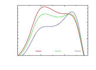
The function is reported in Fig. 2 for and two selected values of temperature. A crucial observation is that does not depend on density. It is seen that in these cases, has two local maxima separated by a local minimum. Let us give the following definitions, illustrated in Fig. 2:
| (7) |
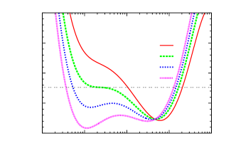
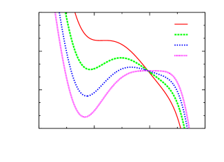
we also consider the analytic continuations of these densities when they exist. Therefore in some range of densities Eq. (5) has four solutions: two of them (the first and the third, upon increasing ) correspond to local minima and the two others correspond to local maxima of the Franz-Parisi potential. This is illustrated in Fig. 3, and remember that while does not depend on density, does. The two local minima correspond to two different metastable glass states, and we call them the attractive glass (the one with smaller ) and repulsive glass (with larger ). Therefore, in this region of density we have coexistence between the two glasses.
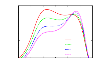
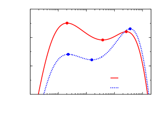
To obtain the phase diagram we must analyze the behavior of systematically as a function of temperature. From Fig. 2 we deduce the existence of several different temperature ranges:
-
•
For , has a unique maximum at small , corresponding to . The other two densities in (7) do not exist, only the attractive glass exists for these temperatures, in the region .
- •
-
•
For , there are two local maxima separated by a local minimum, and the maximum at small is higher. In other words, . In this region the attractive glass exists for , while the repulsive glass exists for . The Franz-Parisi potential is reported in Fig. 3(right).
- •
-
•
For the situation is reversed, , but for the rest nothing changes. The Franz-Parisi potential is in Fig. 3(left).
- •
-
•
Finally, for there is a unique maximum at large corresponding to the attractive glass, which is the only state in this region and exists for .
In Fig. 6 we show the transition lines in the phase diagram that delimit the regions defined above. The two lines and cross each other at point . Below , the liquid-glass transition is given by and the liquid transforms into the attractive glass, while above , the liquid-glass transition is given by and the liquid transforms into the repulsive glass. Hence
| (8) |
and the liquid is ergodic for .
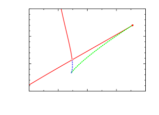
For , the system is arrested but the two different glass phases can exist. The line can be continued from point to point where it merges with the line . The point is a critical endpoint representing a cusp singularity that corresponds to a very singular point of the Franz-Parisi potential. Similarly, the line can be continued from point to point where it merges with the line . Together, these three lines delimit the region of temperature and density where the two glasses coexist, while outside this region only one glass is present. This scenario is the standard one associated with a first order phase transition between the two glasses, as described by the Franz-Parisi potential that exhibits two stable minima in the coexistence region.
3.3 The sticky limit
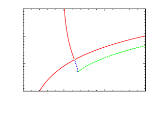
It is interesting to consider a sticky sphere limit where while is kept constant. In this limit the control parameters are therefore and . One can show (A) that in this limit the small- maximum of , corresponding to the attractive glass, moves to . Because of the sticky attraction, particles do not move at all in the attractive glass phase. The height of this maximum can be computed explicitly and gives , see Eq. (26). Hence in this case the spinodal point of the attractive glass can be computed analytically and reaches arbitrarily large densities, therefore the point moves to infinite density. Still, the other two lines and –corresponding respectively to the large- local maximum and the local minimum– have to be computed numerically. The resulting phase diagram is reported in Fig. 7.
3.4 The evolution of the phase diagram with : and singularities
We now summarize the evolution of the phase diagram when the range of the attraction is changed. At large , the phase diagram displays a single re-entrant liquid-glass transition line, see Fig. 1. At very small , a phase coexistence region between two glasses is observed, and is delimited by the triangle -- in Fig. 6. This triangle is quite large at very small (its size diverges in the sticky limit, see Fig. 7). Its size decreases with increasing , until it disappears at where the three points -- merge into a further higher-order singularity of type , also known as swallowtail bifurcation.
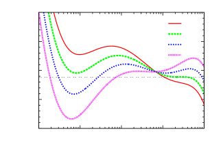
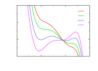
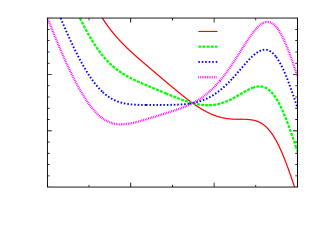
The higher-order singularities, and , are special singular points of the Franz-Parisi potential. From Eq. (4) it is easy to show that if Eq. (5) is satisfied (i.e. on stationary points of the potential), the vanishing of the -th derivative of leads to the vanishing of the -th derivative of . On the points , the first two derivatives of vanish (see Fig. 4) and therefore the first three derivatives of the Franz-Parisi potential vanish (see Fig. 5). On the point , the first three derivatives of vanish and therefore the first four derivatives of the Franz-Parisi potential vanish (not shown). This higher-order singularities lead to peculiar properties of the relaxation dynamics, that have been explored in great detail in the Mode-Coupling theory framework [61, 17, 20, 28, 62] and numerically [63, 64]. However, note that point is a maximum of the Franz-Parisi potential and therefore it is unstable, see Fig. 5(top). This instability has also been discussed within Mode-Coupling Theory [62].
3.5 The Kauzmann transition
Finally, it is important to stress that the complexity contains a term proportional to , which makes it positive for all finite values of . Hence the Kauzmann transition happens at and [36] and it is therefore out of the range of the phase diagrams discussed above. In particular, this implies that the Kauzmann transition always happens in a region of the phase diagram where there is no coexistence between different glasses. The complexity associated to both glasses is therefore positive and for this reason we did not discuss the Kauzmann transition.
4 Conclusion
The main result of this paper is that a static replica picture based on the Franz-Parisi potential allows to re-derive many of the results that have been previously obtained using Mode-Coupling theory for attractive colloids [20, 12, 62], namely the re-entrance of the glass transition line and the coexistence of two glass phases for very short range attractions. Here we limited ourselves to the limit where computations are easier and the replica theory is exact [13], but the computations can in principle be generalized to any finite dimension [36]. Moreover, we found that for suitable attraction range and temperature , the fluid phase extends to density . This shows that sphere packings exist up to packing fraction and can be produced by slow compression of the fluid phase of attractive systems with the above parameters.
Let us conclude by some speculations on the connection between the static replica picture presented in this paper and the dynamic MCT picture of [20, 12, 62], and by presenting some perspective for future work.
4.1 Dynamics
It is very important to discuss the consequences that the static phase diagram obtained above has for dynamics. This is crucial to compare theory with numerical simulations and experiments, that in the glass phase are necessarily out of equilibrium. In simple spin glass models this connection is perfectly understood (both at equilibrium and out of equilibrium) within the general RFOT framework [49, 50, 51, 65, 66, 27]. Unfortunately, when one tries to translate this to approximate theories of particle systems based on MCT and replicas, the situation is much more complicated and controversial results have been obtained in the past [49, 67, 68, 69, 36, 9]. This is due to the fact that, although the general RFOT picture is perfectly consistent at least for large enough dimensions [70], its practical implementation using liquid theory approximate closure can lead to inconsistencies (a fact which is well known in the theory of simple liquids [71]).
Moreover, the discussion of out of equilibrium dynamics is not obvious because in general this dynamics depends a lot on the preparation history and the protocol that is used to explore the glass phase. This is particularly true in the present situation where two distinct glass phases can coexist. In principle, if one considers a slow annealing in the glass phase, one can obtain precise information through the so-called state-following method [48]. However, such a computation goes beyond the scope of this work.
Given these important remarks, we can discuss qualitatively the evolution of the cage radius in the glass phase based on our results for the Franz-Parisi potential. When , the system is in a liquid phase and it is ergodic. Particles can diffuse and the long time limit of connected density correlations is zero. As usual, when from below, dynamics slows down until at diffusion is arrested and the long time limit of the mean square displacement becomes equal to a constant according to Eq. (2). For densities very close to , the mean square displacement plotted as a function of time exhibits a long plateau before crossing over to the diffusive regime, and the value of this plateau corresponds roughly to the long time mean square displacement in the glass phase.
We therefore have two different behavior depending on temperature. When , the liquid arrests into the attractive glass and the value of mean square displacement corresponds to the small solution. Instead, when the liquid arrests into the repulsive glass with larger .
Suppose that we now continue to compress the system slowly and isothermally, out of equilibrium into the glass phase. We have several possibilities:
-
•
At low , the system jumps in the attractive glass at . Then it remains in this phase upon compression. This is because, even if the repulsive glass solution can appear in some range of density, dynamics is arrested in the attractive glass, which does not have a spinodal that could make it unstable. Therefore the blue and green lines in Fig. 6 cannot be observed under isothermal compression below .
-
•
At intermediate temperature the system is stuck in the repulsive glass at . However upon further increasing density, the repulsive glass solution disappears at large enough density (corresponding to , the green line in Fig. 6). Around this point, the system undergoes a transition to the attractive glass, which then remains stable upon further compression. Note however that strong history dependent out of equilibrium effects are surely present, therefore the transition can happen everywhere between the red and green lines in Fig. 6.
-
•
At , there is no attractive glass. The system jumps into the repulsive glass at and remains there at any other density because this is the only solution.
In general, it is reasonable to expect that the repulsive glass phase will be very hard to observe below . Although this phase exists in a strictly mean-field picture as a metastable minimum, one can easily see from Fig. 3(bottom) that the barriers separating this phase from the liquid and the attractive glass are very small. It is therefore most probable that in finite dimensions these barriers are easily crossed in this region, leading to a very short lifetime of the repulsive glass. The most relevant line in the triangle in Fig. 6 seems therefore the line -, consistently with MCT results [20, 62].
In particular, the singularity corresponds to the point where the repulsive glass disappears leading to a local quartic maximum of the Franz-Parisi potential, as shown by the curve for in Fig. 5(top): it is therefore dynamically unobservable as the repulsive glass will always be unstable around this singularity. This is consistent with results from MCT [62]. On the contrary, the singularity corresponds to a local quartic minimum of the Franz-Parisi potential, see the curve for in Fig. 5(bottom). This leads to a unique glass phase with peculiar dynamical properties and a very slow logarithmic relaxation, as it has been shown within MCT [62].
4.2 Perspectives
The discussion of dynamics reported above is very qualitative and preliminary. Exploring further the connection between static and dynamical pictures will surely lead to a better understanding of the rich out of equilibrium dynamics in the glass-glass coexistence phase, where one could naturally expect hysteresis effects. We believe that such a study is a very interesting subject for future work. Performing numerical simulations in high dimensions, following [9], could be very useful to remove undesired metastability effects that complicate the picture. Of course, the hope is to put back these effects in a controlled way once the mean field picture is fully understood.
Our work opens the way to several other studies. First of all one should understand better the nature of the glass phase close to the glass-glass transition. It is to be expected that the complexity function will have two distinct branches, corresponding to the two different sets of glassy states in coexistence. The solution that maximizes the complexity should then correspond to the “typical” phase, in which equilibrium configurations will be found with probability 1 in the thermodynamic limit. This corresponds as usual to choosing the solution that minimizes the Franz-Parisi potential and would provide an “equilibrium” definition of the glass-glass transition line in the coexistence region. How activated barrier processes change the picture within RFOT theory remains an open problem that would be very interesting to investigate. Another question that would be important to address is the role of the Kauzmann transition in finite dimension, which we did not discuss here because in the limit this transition moves at infinite , and is therefore outside the range of relevant densities for the glass-glass coexistence region. Furthermore, one could compute the equation of state of the two glasses, the jump of specific heat at the glass transition, and so on.
For soft matter applications, one would like of course to repeat this calculation in . We expect that the qualitative phase diagram will remain the same in low dimensions. Unfortunately, for the moment the small cage expansion scheme does not give good quantitative results for the dynamical transition in low dimensions, but there is hope to improve it.
For algorithmic applications, it would be very important to perform a “state following” calculation [48], to study how much the states at can be compressed adiabatically: this would give the true threshold beyond which packings cannot be constructed in polynomial time by simulated annealing.
Acknowledgments –
We warmly thank P. Charbonneau and E. Zaccarelli for stimulating discussions.
Appendix A Gaussian replica equations for a generic potential
We collect here all the equations that are needed to obtain the results presented in this work. Because these are based on extensions of previous work [36, 60], we do not provide the general derivation but rather highlight the extensions that are needed with respect to the previous works.
We assume that the potential has a soft repulsive core of diameter . The most general potential we consider has the form
| (9) |
Here is temperature and . We define and and where is the packing fraction of the repulsive core. We also define .
A.1 Finite dimensions
The approximation scheme used here holds for large enough and is based on [60, Eq. (22) and (23)], which give the replicated free entropy separated between the harmonic and the liquid contributions
| (10) |
for replicas at temperature , in a Gaussian cage of variance . The function is defined in [60, just after Eq. (16)] where is a normalized and centered Gaussian of variance , and is the contact value of the hard-spheres cavity function. Introducing bipolar coordinates, as in [36, Appendix C.2.a], we obtain the generalization of [36, Eq. (C16)] to a generic potential
| (11) |
From the replicated entropy we can obtain the Franz-Parisi potential
| (12) |
Note that the Franz-Parisi potential corresponds to the complexity at as a function of .
The local minima of correspond to stable glass phases. Because is independent of at , one can show that the stationary points in of are the same as those of for . In general, the stationary points of are given by the condition
| (13) |
A.2 Infinite dimension
We follow [36]: in the limit of infinite dimension, we are interested in the scaling . One can show that
| (14) |
Using this result in (11), we have
| (15) |
Changing variables again to and and using
| (16) |
we get
| (17) |
We can use this result to compute :
| (18) |
where .
The equation for is
| (19) |
At the equation is
| (20) |
hence the dynamical transition is reached when , as stated in Eq. (6). The non-trivial part of the Franz-Parisi potential, for , is proportional to
| (21) |
A.3 Square-well potential
We consider here the case corresponding to a square well potential. In this case the function is
| (22) |
which allow one to compute easily and solve the equation for .
A.4 Sticky spheres
A special case is the limit and with or . In this case
| (23) |
In this limit the attractive glass has , hence it is useful to compute the limit . We have
| (24) |
hence we can write, with :
| (25) |
The branch of the dynamical transition that corresponds to the attractive glass therefore reads
| (26) |
References
- [1] Torquato S and Stillinger F H 2010 Rev. Mod. Phys. 82 2633–2672
- [2] Rivas G, Ferrone F and Herzfeld J 2004 EMBO Rep. 5 23–27
- [3] Hamming R W 1997 The Art of Doing Science and Engineering (Gordon and Breach)
- [4] Conway J H and Sloane N J A 1993 Sphere Packings, Lattices and Groups (New York: Spriger-Verlag)
- [5] Cohn H 2010 Proceedings of the International Congress of Mathematicians IV 2416–2443 (Preprint arXiv:1003.3053)
- [6] Torquato S and Jiao Y 2010 Physical Review E 82 061302
- [7] Andreanov A and Scardicchio A 2012 Physical Review E 86 041117
- [8] Marcotte E and Torquato S 2013 arXiv.org:1304.5003
- [9] Charbonneau P, Ikeda A, Parisi G and Zamponi F 2011 Phys. Rev. Lett. 107(18) 185702
- [10] Van der Waals J D 1873 Doctoral thesis
- [11] Bernal J and Mason J 1960 Nature 188 910–911
- [12] Sciortino F 2002 Nature materials 1 145
- [13] Kurchan J, Parisi G and Zamponi F 2012 Journal of Statistical Mechanics: Theory and Experiment 2012 P10012
- [14] Sellitto M and Zamponi F 2013 arXiv.org:1306.2912, to appear on Europhysics Letters
- [15] Franz S and Parisi G 1998 Physica A: Statistical Mechanics and its Applications 261 317–339
- [16] Frisch H L and Percus J K 1999 Phys. Rev. E 60 2942–2948
- [17] Fabbian L, Götze W, Sciortino F, Tartaglia P and Thiery F 1999 Phys. Rev. E 59(2) R1347–R1350
- [18] Zaccarelli E and Poon W C 2009 Proceedings of the National Academy of Sciences 106 15203–15208
- [19] Foffi G, Sciortino F, Zaccarelli E and Tartaglia P 2004 Journal of Physics: Condensed Matter 16 S3791
- [20] Dawson K, Foffi G, Fuchs M, Götze W, Sciortino F, Sperl M, Tartaglia P, Voigtmann T and Zaccarelli E 2000 Phys. Rev. E 63(1) 011401
- [21] Eckert T and Bartsch E 2002 Phys. Rev. Lett. 89(12) 125701
- [22] Pham K N, Puertas A M, Bergenholtz J, Egelhaaf S U, Moussaıd A, Pusey P N, Schofield A B, Cates M E, Fuchs M and Poon W C 2002 Science 296 104–106
- [23] Sellitto M, De Martino D, Caccioli F and Arenzon J J 2010 Phys. Rev. Lett. 105 265704
- [24] Sellitto M 2012 Phys. Rev. E 86 030502
- [25] Kirkpatrick T R and Thirumalai D 1987 Phys. Rev. Lett. 58 2091–2094
- [26] Kirkpatrick T R and Wolynes P G 1987 Phys. Rev. B 36 8552–8564
- [27] Wolynes P and Lubchenko V (eds) 2012 Structural Glasses and Supercooled Liquids: Theory, Experiment, and Applications (Wiley)
- [28] Caiazzo A, Coniglio A and Nicodemi M 2004 Phys. Rev. Lett. 93(21) 215701
- [29] Crisanti A and Leuzzi L 2006 Phys. Rev. B 73(1) 014412
- [30] Krakoviack V 2007 Phys. Rev. B 76(13) 136401
- [31] Crisanti A and Leuzzi L 2007 Phys. Rev. B 76(13) 136402
- [32] Krzakala F, Tarzia M and Zdeborová L 2008 Physical Review Letters 101 165702 (pages 4)
- [33] Mézard M and Parisi G 1999 The Journal of Chemical Physics 111 1076–1095
- [34] Franz S, Parisi G, Ricci-Tersenghi F and Rizzo T 2011 The European Physical Journal E 34 1–17
- [35] Velenich A, Parola A and Reatto L 2006 Physical Review E 74 021410 (pages 7)
- [36] Parisi G and Zamponi F 2010 Rev. Mod. Phys. 82 789–845
- [37] Lubachevsky B D and Stillinger F H 1990 J. Stat. Phys. 60 561–583
- [38] Skoge M, Donev A, Stillinger F H and Torquato S 2006 Physical Review E 74 041127 (pages 11)
- [39] van Meel J A, Charbonneau B, Fortini A and Charbonneau P 2009 Phys. Rev. E 80 061110
- [40] Vance S 2011 Advances in Mathematics 227 2144 – 2156
- [41] Ball K 1992 International Math. Research Notices 1992 217–221
- [42] Kabatiansky G A and Levensthein V I 1978 Problems on Information Transmission 14 1–17
- [43] Parisi G and Zamponi F 2006 Journal of Statistical Mechanics: Theory and Experiment 2006 P03017
- [44] Montanari A and Semerjian G 2006 J.Stat.Phys. 125 23–54
- [45] Charbonneau P, Corwin E I, Parisi G and Zamponi F 2012 Phys. Rev. Lett. 109(20) 205501
- [46] Zdeborová L and Krzakala F 2007 Physical Review E 76 031131 (pages 29)
- [47] Krzakala F and Kurchan J 2007 Physical Review E 76 021122 (pages 13)
- [48] Krzakala F and Zdeborová L 2010 EPL (Europhysics Letters) 90 66002
- [49] Kirkpatrick T R and Wolynes P G 1987 Phys. Rev. A 35 3072–3080
- [50] Kirkpatrick T R and Thirumalai D 1988 Phys. Rev. A 37(11) 4439–4448
- [51] Kirkpatrick T R and Thirumalai D 1989 Journal of Physics A: Mathematical and General 22 L149
- [52] Franz S and Parisi G 1995 Journal de Physique I 5 1401–1415
- [53] Franz S and Parisi G 1997 Phys. Rev. Lett. 79 2486–2489
- [54] Cardenas M, Franz S and Parisi G 1998 Journal of Physics A: Mathematical and General 31 L163–L169
- [55] Monasson R 1995 Phys. Rev. Lett. 75 2847–2850
- [56] Dawson K A, Franz S and Sellitto M 2003 Europhysics Letters 64 302–308
- [57] Cammarota C, Cavagna A, Giardina I, Gradenigo G, Grigera T S, Parisi G and Verrocchio P 2010 Phys. Rev. Lett. 105(5) 055703
- [58] Mézard M and Parisi G 1996 Journal of Physics A: Mathematical and General 29 6515
- [59] Mezard M and Parisi G 2012 Structural Glasses and Supercooled Liquids: Theory, Experiment and Applications ed PGWolynes and VLubchenko (Wiley & Sons) (Preprint arXiv:0910.2838)
- [60] Berthier L, Jacquin H and Zamponi F 2011 Phys. Rev. E 84(5) 051103
- [61] Bergenholtz J and Fuchs M 1999 Phys. Rev. E 59(5) 5706–5715
- [62] Götze W 2009 Complex dynamics of glass-forming liquids: A mode-coupling theory (Oxford University Press, USA)
- [63] Sciortino F, Tartaglia P and Zaccarelli E 2003 Phys. Rev. Lett. 91(26) 268301
- [64] Charbonneau P and Reichman D R 2007 Phys. Rev. Lett. 99(13) 135701
- [65] Cugliandolo L F and Kurchan J 1993 Phys. Rev. Lett. 71 173–176
- [66] Castellani T and Cavagna A 2005 Journal of Statistical Mechanics: Theory and Experiment 2005 P05012
- [67] Ikeda A and Miyazaki K 2010 Phys. Rev. Lett. 104 255704
- [68] Schmid B and Schilling R 2010 Phys. Rev. E 81 041502
- [69] Szamel G 2010 Europhysics Letters 91 56004
- [70] Charbonneau P, Ikeda A, Parisi G and Zamponi F 2012 Proceedings of the National Academy of Sciences 109 13939–13943
- [71] Hansen J P and McDonald I R 1986 Theory of simple liquids (London: Academic Press)