Impedance and Scattering Variance Ratios of Complicated Wave Scattering Systems in the Low Loss Regime

Abstract

Random matrix theory (RMT) successfully predicts universal statistical properties of complicated wave scattering systems in the semiclassical limit, while the random coupling model offers a complete statistical model with a simple additive formula in terms of impedance to combine the predictions of RMT and nonuniversal system-specific features. The statistics of measured wave properties generally have nonuniversal features. However, ratios of the variances of elements of the impedance matrix are predicted to be independent of such nonuniversal features and thus should be universal functions of the overall system loss. In contrast with impedance variance ratios, scattering variance ratios depends on nonuniversal features unless the system is in the high loss regime. In this paper, we present numerical tests of the predicted universal impedance variance ratios and show that an insufficient sample size can lead to apparent deviation from the theory, particularly in the low loss regime. Experimental tests are carried out in three two-port microwave cavities with varied loss parameters, including a novel experimental system with a superconducting microwave billiard, to test the variance-ratio predictions in the low loss time-reversal-invariant regime. It is found that the experimental results agree with the theoretical predictions to the extent permitted by the finite sample size.

PACS numbers: 05.45.Mt 24.60.-k 42.25.Dd 78.20.Bh

I Introduction

Understanding the properties of complicated wave scattering systems Newton1966B is a common challenge in many engineering and physics fields, such as quantum chaotic systems Stockmann1999B ; Haake2000B , quantum dots and mesoscopic systems Altshuler1991B ; Brouwer1997 ; Alhassid2000 ; Mello2004B , acoustic waves Pagneux2001 , and microwave cavities Doron1990 ; Kuhl2005 ; Hemmady2005a ; Hemmady2005b . Due to the complexity of wave propagation and scattering in many of these systems, numerically solving the wave equations with high resolution is difficult or impractical. This is particularly true when the wavelength is short compared to the characteristic size of the scattering region (the situation of interest in this paper). In addition, in this case, scattering properties are extremely sensitive to small changes in system parameters, which may not be precisely known. Thus, a statistical approach has become a popular alternative for describing the wave properties Holland1999B .

Researchers have developed statistical models based on random matrix theory (RMT), which successfully predict certain universal statistical properties of complicated wave scattering systems Bohigas1984 ; Mehta1991B ; Akemann2011B . In order to apply RMT to practical wave systems, one usually needs to account for nonuniversal system-specific features, which are not included in RMT. For example, considering microwave signals entering an enclosure through localized ports and propagating inside, the port coupling between the enclosure and the outside world is one system-specific feature Zheng2006a ; Zheng2006b . The short ray trajectories between ports due to scattering from fixed walls and/or objects within the enclosure are also nonuniversal system-specific features Hart2009 .

The random coupling model (RCM) is a well-developed model to combine the universal predictions of RMT and the nonuniversal features of a practical system by a simple additive formula in terms of impedance Zheng2006a ; Zheng2006b ; Hart2009 . This model has been experimentally verified in microwave cavities, and it offers a complete statistical model for the impedance matrices, the scattering matrices Hemmady2005a ; Hemmady2005b ; Yeh2010a ; Yeh2010b , the admittance matrices Hemmady2006a , the conductances Hemmady2006c , and the fading statistics Yeh2012a ; Yeh2012b of practical systems. The statistical distributions of the universal predictions of RMT and the practical distributions which includes nonuniversal features are distinctly different for most wave scattering properties. However, the impedance variance ratio (defined below) is a quantity that is predicted to be independent of nonuniversal features of the wave system, and it is expected to be a universal function of the loss of the system Zheng2006c . In this paper, we use “universality” to mean that the impedance variance ratio is independent of the system-specific features including the port coupling of the system and the short ray trajectories betweeen ports.

Impedance is a meaningful concept in electromagnetism, and it can be extended to all wave scattering systems. In a linear electromagnetic wave system with $N$ ports, the $N\times N$ impedance matrix Z is the linear relationship of the complex phasor voltage vector $\widehat{\textbf{{V}}}$ of the $N$ port voltages and the complex phasor current vector $\widehat{\textbf{{I}}}$ of the $N$ port currents, via the phasor generalization of Ohm’s law as $\widehat{\textit{{V}}}=\textbf{Z}\widehat{\textit{{I}}}$ Pozar1990B . A quantum-mechanical quantity corresponding to the impedance is the so-called reaction matrix, which is often denoted in the literature as K and is related to Z by $\textbf{K}=-i\textbf{Z}$ Alhassid2000 ; Verbaarschot1985 ; Lewenkopf1991 ; Beck2003 ; Fyodorov2004 ; Fyodorov2005 ; Savin2005 . The impedance matrix can also be related to the scattering matrix S via the relationship Zheng2006a ; Zheng2006b

$$\textbf{Z}=\textbf{Z}_{0}^{1/2}\left(\textbf{1}+\textbf{S}\right)\left(\textbf{1}-\textbf{S}\right)^{-1}\textbf{Z}_{0}^{1/2},$$ (1)

where $\textbf{Z}_{0}$ is a $N\times N$ diagonal matrix whose diagonal element $Z_{0,nn}$ is the characteristic impedance of the n^th scattering channel mode, and 1 is the identity matrix. The scattering matrix S specifies the linear relationship between the incoming wave vector $\widehat{\textit{{a}}}$ and the outgoing wave vector $\widehat{\textit{{b}}}$, as $\widehat{\textit{{b}}}=\textbf{S}\widehat{\textit{{a}}}$. The $n^{th}$ element of the incoming and outgoing power waves are $a_{n}=(V_{n}+Z_{0,nn}I_{n})/\sqrt{Z_{0,nn}}$ and $b_{n}=(V_{n}-Z_{0,nn}I_{n})/\sqrt{Z_{0,nn}}$, where $V_{n}$ and $I_{n}$ are the voltage and current at the $n^{th}$ port, respectively Pozar1990B , and the incident and reflected power fluxes in channel $n$ are $|a_{n}|^{2}$ and $|b_{n}|^{2}$.

For complicated wave scattering systems, the impedance matrices and the scattering matrices are sensitive to small variations of the system, such as change of the applied frequency, the configuration of the enclosure boundary, or the location and orientation of an internal scatterer. The statistical variations of the elements of Z and S due to small random changes in the scattering system are of great interest Zheng2006c ; Fyodorov2005 ; Savin2006 . For example, the variances of the the elements of S and their ratio (the Hauser-Feshbach relation) have been studied in the nuclear scattering literature when researchers investigate the statistics of inelastic scattering of neutrons Hauser1952 and compound nuclear reactions Verbaarschot1985 ; Agassi1975 . Friedman and Mello used information theory to derive the Hauser-Feshbach formula in the statistical treatment of nuclear reactions Friedman1985 .

The elastic enhancement factor is the ratio of variances in reflection (diagonal elements of S) to that in transmission (off-diagonal elements of S) Verbaarschot1986 . In chaotic scattering, elastic processes (the diagonal elements) are known to be systematically enhanced over inelastic ones (the off-diagonal elements) Kretschmer1978 ; Dietz2010 . For a two-port system, the elastic enhancement factor $W=\sqrt{\textrm{Var}[S_{11}]\textrm{Var}[S_{22}]}/\textrm{Var}[S_{12}]$, where $\textrm{Var}[x]$ stands for the variance of the variable $x$, and $S_{ij}$ denotes the matrix element of S that occupies the $i^{th}$ row and the $j^{th}$ column. In research on electromagnetic fields in mode-stirred reverberating chambers, Fiachetti and Michelsen have conjectured the universality of the ratio of the variances of the scattering elements in the cases of time reversal invariant systems (corresponding to RMT of the Gaussian orthogonal ensemble (GOE)) Fiachetti2003 . The universality of the scattering variance ratio has been tested with wave scattering experiments in microwave resonators in the GOE case Zheng2006c . Dietz et al. have also tested the universality of the elastic enhancement factor with microwave resonators in the GOE case and in the cases of partially breaking of time reversal invariance (corresponding to RMT of the Gaussian unitary ensemble (GUE)) Dietz2010 . Ławniczak et al. have used microwave networks to test the elastic enhancement factor in both the GOE and GUE cases Lawniczak2010 ; Lawniczak2011 ; Lawniczak2012 .

In this paper we are concerned with the impedance variance ratio, which is defined as Zheng2006c

$$\Xi_{Z}\equiv\frac{\textrm{Var}[Z_{ij}]}{\sqrt{\textrm{Var}[Z_{ii}]\textrm{Var}[Z_{jj}]}},\ \ \ i\neq j,$$ (2)

and the scattering variance ratio, defined as

$$\Xi_{S}\equiv\frac{\textrm{Var}[S_{ij}]}{\sqrt{\textrm{Var}[S_{ii}]\textrm{Var}[S_{jj}]}},\ \ \ i\neq j,$$ (3)

where the variances arise from small variations of the system. For a reciprocal ($Z_{ij}=Z_{ji}$) two-port system, the impedance variance ratio is $\Xi_{Z}=\textrm{Var}[Z_{12}]/\sqrt{\textrm{Var}[Z_{11}]\textrm{Var}[Z_{22}]}$. Similarly, the scattering variance ratio is $\Xi_{S}=\textrm{Var}[S_{12}]/\sqrt{\textrm{Var}[S_{11}]\textrm{Var}[S_{22}]}$. Note that $\Xi_{S}$ is the inverse of the elastic enhancement factor of a two-port system. The impedance variance ratio $\Xi_{Z}$ is predicted to be a universal function of the loss parameter $\alpha$ Zheng2006c , which characterizes the losses and mode-spacing within the wave scattering system (defined below). On the other hand, $\Xi_{S}$ is in general dependent on the system-specific features of the wave scattering system and hence not universal. Only in the high loss regime ($\alpha\gg 1$) can one assume that the fluctuating part of the impedance matrix (or the scattering matrix) is much smaller than the mean part, which allows one can obtain the result $\Xi_{S}\simeq\Xi_{Z}$ ($\alpha\gg 1$) Zheng2006c , which implies that $\Xi_{S}$ is approximately universal for high loss.

The loss parameter can be understood as the degree of overlap of resonances in frequency in the electromagnetic case (or energy level in the quantum case) due to the distributed losses of the closed version of the wave scattering system. For example, in the case of electromagnetic wave scattering, the loss parameter is

$$\alpha=\frac{f}{2Q\Delta f},$$ (4)

where $f$ is the frequency of the wave signal, $\Delta f$ is the average spacing between cavity resonant frequencies near $f$, and $Q$ is the quality factor due to the distributed losses of the closed cavity, such as losses from conducting walls or a lossy dielectric that fills the cavity Hemmady2005a ; Zheng2006a ; Zheng2006b . Based on RMT, researchers have given analytical expressions of $\Xi_{Z}(\alpha)$ Zheng2006c ; Fyodorov2005 and $\Xi_{S}(\alpha)$ Fyodorov2005 ; Savin2006 for the GOE and GUE cases. In this paper, we focus on the time reversal invariant case (GOE).

The goal of this paper is to experimentally test the analytical predictions of the impedance variance ratio and the scattering variance ratio in the low loss regime. Dietz et al. carried out experiments in the low loss regime, but their interests were in the elastic enhancement factor (inverse of $\Xi_{S}$) in the weak port-coupling situation Dietz2010 . Note that the common approach to accounting for coupling (one nonuniversal feature) is to use a single scalar quantity for a given frequency range (the amplitude of the averaged scattering parameter $|\overline{S_{ii}}|$) Kuhl2005 ; Savin2006 , whereas the random coupling model treats nonuniversal features more generally by using a complex function of frequency (the frequency-dependent averaged impedance matrix, defined in Section 2.2), and includes short ray trajectories. Zheng et al.’s study of $\Xi_{Z}$ and $\Xi_{S}$ Zheng2006c and Ławniczak et al.’s study of the elastic enhancement factor Lawniczak2010 ; Lawniczak2011 ; Lawniczak2012 applied the original version of the RCM to take account of the nonuniversality of the port-coupling. In this paper we apply the extended version of the RCM to further include the nonuniversal features of the short ray trajectories. We also test the low loss regime which has not been previously achieved by Zheng’s or Ławniczak’s experiments Zheng2006c ; Lawniczak2010 ; Lawniczak2011 ; Lawniczak2012 .

In the following sections, we first review the theory and present numerical tests of $\Xi_{Z}$ and $\Xi_{S}$ as a function of loss parameter. The numerical tests point out a numerical deviation from the theory due to the finite number of samples, which is more significant in the low loss regime for the impedance variance ratio. After the numerical tests, we present our experimental systems of three microwave cavities with varied values of the loss parameter and make a thorough experimental test in a broad range of loss parameters.

II Theory and Numerical Results

II.1 Universal Statistics Based on RMT

The theoretical model of the impedance variance ratio $\Xi_{Z}$ is derived from RMT Zheng2006c . Using RMT, for a complicated wave scattering system with time reversal invariance of wave propagation, researchers have developed a statistical model of the impedance matrix $\textbf{Z}_{rmt}$ Zheng2006a ; Zheng2006b ; Hart2009 ; Lewenkopf1991 ; Beck2003 ; Fyodorov2004 ; Fyodorov2005 ; Savin2005 . This statistical model is applicable to situations where system-specific short-ray-trajectory effects are negligible and the ports are such that the input-output channels are perfectly matched to the scatterer (in the sense that $\langle\textbf{Z}\rangle=\textbf{1}$, where $\langle\ldots\rangle$ denotes a suitable ensemble average).

With the known statistics of $\textbf{Z}_{rmt}$, the impedance variance ratio as a function of $\alpha$ can be analytically derived Mehta1991B ; Zheng2006a

$$\Xi_{Z_{rmt}}(\alpha)=\left[3-2\int_{0}^{\infty}\frac{4\ g(x)}{4+(x/\alpha)^{2}}\ dx\right]^{-1},$$ (5)

where $\displaystyle g(x)=f^{2}(x)-\left[\int^{x}_{0}f(x^{\prime})dx^{\prime}-\frac{1}{2}\right]\frac{df}{dx}$ and $\displaystyle f(x)=\frac{\sin(\pi x)}{\pi x}$ in the time reversal invariant case. This result is shown as the thick black curve in Fig.  1, where the loss parameter scale is logarithmic. Note that $\Xi_{Z_{rmt}}=1/3$ in the GOE lossless case ($\alpha=0$) and $\Xi_{Z_{rmt}}=1/2$ as $\alpha\rightarrow\infty$.

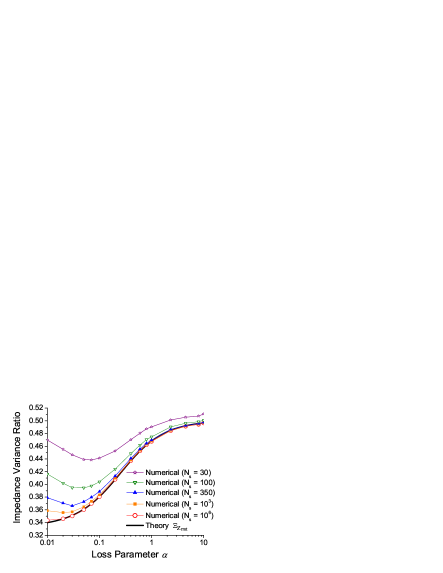
Figure 1: The impedance variance ratio versus the loss parameter $\alpha$. The thick black curve is the analytical formula $\Xi_{Z_{rmt}}$, Eq.  (5). The other colored curves are numerical results of mean impedance variance ratio $\widetilde{\Xi}_{Z_{rmt}}^{(N_{s})}$ based on $\textbf{Z}_{rmt}$ with different numbers of samples ($N_{s}$) indicated in the parentheses.

In addition to the analytical prediction (Eq.  (5)), we also numerically generate $2\times 2$ random impedance matrices $\textbf{Z}_{rmt}$ (using the appropriate RMT ensemble) and compute the variance ratios with different values of the loss parameter $\alpha$. We select 15 different loss parameters from $\alpha=0.01$ to $\alpha=10$. With each loss parameter, we generate a finite ensemble with $N_{s}$ samples of $\textbf{Z}_{rmt}$ matrices. The variations of these matrices represent a finite sampling of the universal variations of the wave scattering system. Because the number of generated sample matrices ($N_{s}$) is finite, the variance ratio $\displaystyle\Xi_{Z_{rmt}}^{(N_{s})}=\frac{\textrm{Var}^{(N_{s})}[Z_{rmt,12}]}{\sqrt{\textrm{Var}^{(N_{s})}[Z_{rmt,11}]\textrm{Var}^{(N_{s})}[Z_{rmt,22}]}}$ of a finite ensemble is not a single value, but has a statistical distribution. To illustrate the finite-sample-size issue, we choose the sample numbers as $N_{s}=$ 30, 100, 350, $10^{3}$, and $10^{6}$ for each loss parameter, and we numerically generate the statistical distribution of $\Xi_{Z_{rmt}}^{(N_{s})}$. We plot the means of these distributions ($\widetilde{\Xi}_{Z_{rmt}}^{(N_{s})}=\langle\Xi_{Z_{rmt}}^{(N_{s})}\rangle$) versus the loss parameter as colored curves in Fig.  1. One can see the deviations between the numerical $\widetilde{\Xi}_{Z_{rmt}}^{(N_{s})}$ and the analytical theory (Eq.  (5)) are more significant in the low loss cases. This indicates that fluctuations of $\Xi_{Z_{rmt}}^{(N_{s})}$ in the low loss cases are more significant, thus necessitating a large number of samples to achieve good agreement between the finite-size numerical mean and the theory.

As with the impedance variance ratio $\Xi_{Z_{rmt}}$, we have done the same analysis for the scattering variance ratio $\Xi_{S_{rmt}}$, where $\textbf{S}_{rmt}=(\textbf{Z}_{rmt}-\textbf{1})(\textbf{Z}_{rmt}+\textbf{1})^{-1}$. For the scattering matrices generated based on RMT in the time reversal invariant (GOE) case, the theoretical prediction is $\Xi_{S_{rmt}}=1/2$ Brouwer1997 ; Zheng2006c , and it is independent of the loss parameter $\alpha$. We show the theory and numerical results in Fig.  2. Note that $\Xi_{S_{rmt}}$ does not contain the nonuniversal features encountered in a typical practical system.

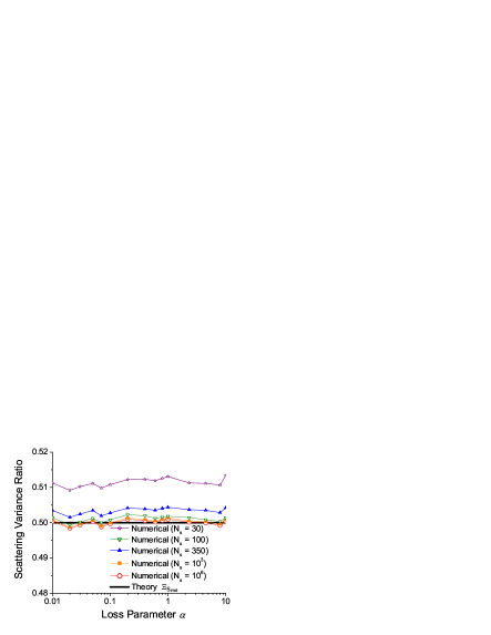
Figure 2: The scattering variance ratio versus the loss parameter $\alpha$. The thick black curve is the theory $\Xi_{S_{rmt}}=1/2$. The other colored curves are numerical results $\widetilde{\Xi}_{S_{rmt}}^{(N_{s})}$ with different numbers of samples ($N_{s}$) indicated in the parentheses.

II.2 Including the Nonuniversal Features through the RCM

To extend the predictions of RMT to practical systems and include nonuniversal features, Zheng et al. have introduced the random coupling model Zheng2006a ; Zheng2006b . The original version of the random coupling model took the system-specific port coupling into account through the radiation impedance matrix. This method has also been applied in previous work on impedance and scattering variance ratios Zheng2006c . Hart et al. have considered the additional system-specific features of short ray trajectories between ports and developed the short-ray-trajectory-corrected version of the RCM Hart2009 . This RCM connects the universal fluctuating part and the practical impedance matrix Z as

$$\textbf{Z}_{n}=\textbf{R}_{avg}^{-1/2}\left(\textbf{Z}-i\textbf{X}_{avg}\right)\textbf{R}_{avg}^{-1/2}.$$ (6)

The normalized impedance matrix $\textbf{Z}_{n}$ represents the universal part, and its statistics are the same as the RMT prediction ($\textbf{Z}_{rmt}$) Yeh2010a ; Yeh2010b . The nonuniversal features of the port coupling (the radiation impedance) and short ray trajectories are included in the ensemble-averaged impedance matrix $\textbf{Z}_{avg}=\textbf{R}_{avg}+i\textbf{X}_{avg}$, where $\textbf{R}_{avg}=\textrm{Re}[\textbf{Z}_{avg}]$, $\textbf{X}_{avg}=\textrm{Im}[\textbf{Z}_{avg}]$ Hart2009 ; Yeh2010b .

In experiments measuring the statistics of wave scattering properties, one needs an ensemble measurement of many different realizations of the system Hemmady2005a ; Yeh2010a ; Yeh2010b ; Schafer2005 ; Schanze2005 . In this paper, our experimental measurement ensemble includes configuration variation and frequency variation. These variations aim to create a set of systems in which none of the nonuniversal system details are reproduced from one realization to another, except for the effects of the port coupling and short ray trajectories. The previous analysis of the experimental results for the impedance variance ratio included frequency-dependent nonuniversal feature of short ray trajectories Zheng2006c . In this paper we remove these by utilizing the extended RCM (Eq.  (6)) Yeh2010a ; Yeh2010b .

Considering the extended RCM (Eq.  (6)), in general the variance ratio $\Xi_{Z}$ of the impedance matrix and the variance ratio $\Xi_{Z_{n}}$ of the normalized impedance matrix are not equal, and their relationship depends on the elements of $\textbf{R}_{avg}$ (note that $\textbf{X}_{avg}$ does not influence the variances of the impedance elements). However, if the ports of the wave scattering system are far apart, then the off-diagonal elements of $\textbf{Z}_{avg}$ are small Zheng2006c , and one can approximately simplify the relationship between $\Xi_{Z}$ and $\Xi_{Z_{n}}$. More specifically for a two-port system, one can define

$$\textbf{R}_{avg}^{1/2}=\left[\begin{array}[]{cc}A&B\\ C&D\\ \end{array}\right],$$ (7)

where $A$, $B$, $C$, and $D$ ($B=C$ in time reversible (reciprocal) cases) are all frequency-dependent real quantities. Under the condition $A$, $D\gg|B|$, $|C|$, the relationships of impedance variances over configuration realizations at a frequency $f$ become

$$\textrm{Var}[Z_{11}]=A^{2}(f)\textrm{Var}[Z_{n,11}],$$ (8)

$$\textrm{Var}[Z_{22}]=D^{2}(f)\textrm{Var}[Z_{n,22}],$$ (9)

$$\textrm{Var}[Z_{12}]=A(f)D(f)\textrm{Var}[Z_{n,12}].$$ (10)

In this case, $A(f)$ and $D(f)$ cancel in the calculation of the variance ratio, and one has the universal result

$$\Xi_{Z}=\Xi_{Z_{n}}.$$ (11)

This equation shows the significance of the impedance variance ratio: if off-diagonal elements of $\textbf{R}_{avg}$ are negligible, the quantity is independent of the system-specific feature $\textbf{Z}_{avg}$ and is directly related to the universal fluctuating quantity $\textbf{Z}_{n}$. The statistics of $\textbf{Z}_{n}$ are the same as the statistics of $\textbf{Z}_{rmt}$, and the statistical properties only depend on the loss parameter $\alpha$ Zheng2006c . Therefore, the impedance variance ratio becomes is a universal property of the wave scattering system and only depends on the loss parameter $\alpha$.

On the other hand, the scattering variance ratio $\Xi_{S}$ of the practical scattering matrix does not have this universality, even under the condition $A$, $D\gg|B|$, $|C|$ Zheng2006c . The elastic enhancement factor (inverse of $\Xi_{S}$) is known to be a function of both the loss parameter $\alpha$ and the coupling, in general Savin2006 . Only in the high loss regime ($\alpha\gg 1$), can one further assume that the fluctuation part of the practical impedance $\delta\textbf{Z}$ is much smaller than the mean part of the practical impedance $\langle\textbf{Z}\rangle$, as $\delta\textbf{Z}\ll\langle\textbf{Z}\rangle$ and the practical impedance elements $|Z_{11}|$, $|Z_{22}|\gg|Z_{12}|$, $|Z_{21}|$, and therefore with Eq.  (1) Zheng et al. have derived Zheng2006c ,

$$\Xi_{S}\simeq\Xi_{Z},\ \ \ \ (\alpha\gg 1).$$ (12)

Note that for the high loss GOE case, $\Xi_{S}\simeq\Xi_{Z}=1/2$.

III Experimental Systems and Results

III.1 Three Experimental Systems

In order to experimentally test the predictions above, we use an Agilent PNA E8364C network analyzer to measure the frequency dependence of the complex $2\times 2$ scattering matrices S of three two-port microwave scattering enclosures in the semiclassical limit. To achieve the semiclassical limit, the typical length scales of the cavities are at least several times larger than the free-space wavelength making the systems sensitive to small perturbations. We add perturbing objects (perturbers) in each wave scattering system and move the perturbers (with the movement larger or on the scale of the applied wavelength) to create an ensemble for each wave scattering system. We can convert S to Z by Eq.  (1), and the characteristic impedances of the transmission lines connected to the ports are $Z_{0,11}=Z_{0,22}=50\ [\Omega]$ in all experiments.

The first experimental system is a quasi-two-dimensional ray-chaotic “$1/4$-bowtie-shaped” microwave billiard illustrated in Fig.  3(a). The cavity is made of copper and has two coupling ports schematically shown as the red dots in Fig.  3(a). Microwaves are injected or extracted through each port antenna attached to a coaxial transmission line, and each antenna is inserted into the cavity through a small hole (diameter about 0.1 [cm]) in the lid, similar to previous setups Yeh2010a ; Hemmady2006a ; Hemmady2006c . Due to the two convex circular arc walls, ray trajectories are chaotic. This system has previously been used to test the predictions of RMT So1995 ; Gokirmak1998 ; Chung2000 . To create an ensemble for statistical analysis, we add two metal perturbers to the interior of the cavity and randomly move the perturbers to create 100 different realizations Yeh2010a ; Yeh2010b . For each realization, we measure the scattering matrix over the frequency window ($6-18$ [GHz]). The perturbers are conducting cylinders of diameter 5.1 [cm] and height approximately equal to that of the cavity (0.7 [cm]).

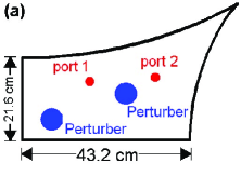
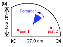
Figure 3: (a) The $1/4$-bowtie cavity with the two ports as red dots and the two metallic perturbers as blue circles. (b) The cut-circle cavity with the two ports as red dots and the Teflon perturber as the blue wedge.

In order to test the predictions of $\Xi_{Z}$ and $\Xi_{S}$ in the low loss regime, we have carried out experiments (similar to the $1/4$-bowtie cavity) in a superconducting microwave cavity, illustrated in Fig.  3(b). The shape of the cavity is a symmetry-reduced “cut-circle” that shows chaos for ray trajectories Yeh2012a ; Ree1999 ; Richter2001 ; Dietz2006 ; Dietz2008 . The superconducting cavity is made of copper with Pb-plated walls and cooled to a temperature (6.6 [K]) below the transition temperature of Pb. A Teflon wedge (the blue wedge in Fig.  3(b)) can be rotated as a ray-splitting perturber inside the cavity, and we rotate the wedge in $5^{o}$ increments to create an ensemble of 72 different realizations. Measurements of the scattering matrix of the superconducting cavity are calibrated by an in-situ broadband cryogenic calibration system (more experimental details of the cryogenic systems can be found in Yeh2013 ).

The previous two wave systems are both quasi-two-dimensional cavities. We also do experiments in a three-dimensional metal cavity, which we call the “GigaBox” Taddese2011 ; Frazier2013 . The GigaBox is approximately a rectangular microwave resonator with dimensions of length 1.27 [m], width 1.22 [m], and height 0.65 [m]. The cavity is made of aluminum and has mode stirrers (a fan formed by aluminum plates) inside it. The mode stirrers and the irregularities on the surface create a complicated wave scattering environment. A stepper motor is used to rotate the mode stirrers to create an ensemble of 199 different realizations.

Table 1: Parameters of the six experimental data sets.

Data Set	I	II	III	IV	V	VI
Cavity	Cut-circle	Cut-circle	$1/4$-bowtie	$1/4$-bowtie	GigaBox	GigaBox
$f_{R}$ [GHz]	$14-16$	$17-19$	$14-16$	$17-19$	$6.0-6.1$	$9.0-9.1$
$\Delta f$ [MHz]	28	23	10	8.6	0.031	0.014
$N_{m}$	71	87	200	230	3200	7100
$N_{r}$	72	72	100	100	199	199
$\alpha$	0.02	0.23	1.24	1.9	4.51	9.31
$\Xi_{Z}$	$0.39\pm 0.01$	$0.44\pm 0.01$	$0.48\pm 0.01$	$0.48\pm 0.01$	$0.502\pm 0.005$	$0.487\pm 0.004$
$\Xi_{Z_{n}}$	$0.37\pm 0.02$	$0.45\pm 0.01$	$0.48\pm 0.01$	$0.48\pm 0.01$	$0.502\pm 0.005$	$0.489\pm 0.004$
$\Xi_{S}$	$0.41\pm 0.01$	$0.48\pm 0.01$	$0.50\pm 0.01$	$0.48\pm 0.01$	$0.508\pm 0.005$	$0.503\pm 0.004$
$\Xi_{S_{n}}$	$0.51\pm 0.02$	$0.55\pm 0.02$	$0.51\pm 0.01$	$0.50\pm 0.01$	$0.503\pm 0.005$	$0.489\pm 0.004$

For each of these three microwave systems, we select two frequency ranges where the condition $A$, $D\gg|B|$, $|C|$ (Eq.  (7)) is satisfied. The parameters of these six experimental data sets are shown in Table 1, where $f_{R}$ is the frequency range, $\Delta f$ is the mean frequency spacing of the resonant modes in that range, $N_{m}$ is the approximate number of modes in the frequency range, $N_{r}$ is the number of configuration realizations. The first data set of the cut-circle cavity is measured at temperature 6.6 [K] (the superconducting case), and the second data set is from the cut-circle cavity at temperature 270 [K] (the normal metal case). Note that the GigaBox system has a much higher mode density than the two quasi-two-dimensional cavities due to its large volume ($V$ = 1.01 [m³]), and therefore the smaller frequency range (100 [MHz]) of the GigaBox contains more resonances than the frequency range (2 [GHz]) of the other two cavities. The loss parameters $\alpha$ for these data sets are determined as the best-fit parameter by the method introduced in Yeh2010b , which compares the statistics of the normalized scattering element $S_{n,12}$ and the prediction of RMT ($S_{rmt,12}$). The averaged variance ratios ($\Xi_{Z}$, $\Xi_{Z_{n}}$, $\Xi_{S}$, and $\Xi_{S_{n}}$) and their standard errors of the mean are calculated from the experimental data, and we introduce the procedures in the next section.

III.2 Analysis of the Variance Ratios

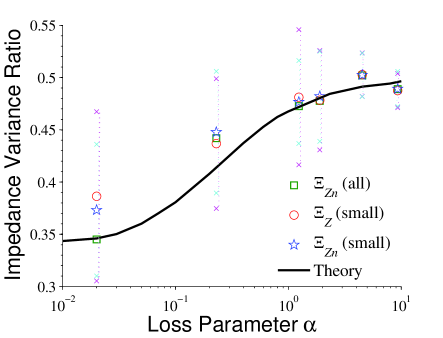
Figure 4: The experimental impedance variance ratio versus the loss parameter $\alpha$. The thick black curve is the analytical formula $\Xi_{Z_{rmt}}$, Eq.  (5). The green squares are $\Xi_{Z_{n}}$ from the normalized impedance matrix over the whole frequency range. The red circles are averaged $\Xi_{Z}$, and the pink bars show the standard deviations of $\Xi_{Z}$ from the practical impedance matrix over the smaller frequency windows. The blue stars are averaged $\Xi_{Z_{n}}$, and the light blue bars show the standard deviations of $\Xi_{Z_{n}}$ from the normalized impedance matrix over the smaller frequency windows.

We show the impedance variance ratios of the normalized impedance matrix $\textbf{Z}_{n}$ and the measured impedance matrix Z versus the loss parameter $\alpha$ in Fig.  4. As shown in the finite-size numerical ensembles (Fig.  1), a large number of samples are critical for accurately determining the impedance variance ratio, especially in the low loss regime. For experimental measurement, the number of samples from different configuration realizations are limited by the remaining correlations in the experimental data. Therefore, we take the samples for computing the variance from the ensemble not only with different configuration realizations but also frequency variations. Note that in Eqs.  (8) to (11) the variances are taken over the configuration realizations at a fixed frequency. However, if $\alpha$ is frequency independent, Maxwell’s equations are invariant to the scaling $f\rightarrow\eta f$ and (length) $\rightarrow\eta$(length), so that a frequency change can be thought of as equivalent to a configuration change.

For the normalized impedance matrix $\textbf{Z}_{n}$, the frequency-dependent nonuniversal features ($A(f)$ and $D(f)$) have been removed by the RCM, so we can compute the impedance variance ratio $\Xi_{Z_{n}}$ from variances over the whole frequency range and all realizations. The results are shown as green squares in Fig.  4. For the measured impedance matrix Z, the frequency-dependent nonuniversal features remain, so taking variances over the whole frequency range is not valid. Therefore, we take a smaller frequency window (1/20 of the whole frequency range $f_{R}$) instead and assume that the nonuniversal features ($A(f)$ and $D(f)$) are approximately constant in this small frequency window (100 [MHz] for the cut-circle cavity and the $1/4$-bowtie cavity, and 5 [MHz] for the GigaBox). With this condition, the derivation from Eqs.  (8) to (11) is still valid. We compute the averaged impedance variance ratio $\Xi_{Z}$ of the 20 impedance variance ratios of the smaller windows and plot the results as red circles in Fig.  4. For comparison, we also plot the averaged impedance variance ratio $\Xi_{Z_{n}}$ of small windows for the normalized impedance matrix as the blue stars. The pink bars (and the light blue bars) show the standard deviations of the 20 variance ratios of the measured (and normalized) impedance matrices for the smaller windows to illustrate the larger fluctuations in the low loss regime. Note that $1/\sqrt{20}$ of these standard deviations are the standard errors of the mean shown in the last four rows in Table 1. Note also that in Fig.  4 the green squares and the blue stars are both computed from the normalized impedance matrix, and the only difference is the finite sample size due to the frequency range for the green squares being 20 times larger than the frequency range for the blue stars. The values of the blue stars are systematically larger than the values of the green squares, especially the lowest loss case. This trend is consistent with the finite-sample-size deviation illustrated in Fig.  1. Comparing all three sets of experimental impedance variance ratios, the results in Fig.  4 agree with the prediction $\Xi_{Z}=\Xi_{Z_{n}}=\Xi_{Z_{rmt}}$ as a function of the loss parameter, to the extent permitted by the finite sample sizes.

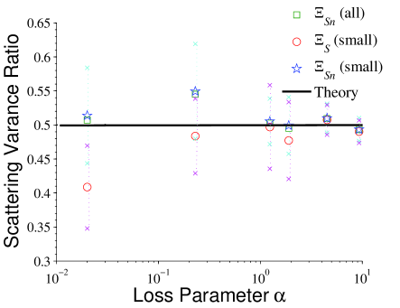
Figure 5: The experimental scattering variance ratio versus the loss parameter $\alpha$. The thick black curve is the theory $\Xi_{S_{rmt}}=1/2$. The green squares are $\Xi_{S_{n}}$ from the normalized scattering matrix over the whole frequency range. The red circles are averaged $\Xi_{S}$, and the pink bars show the standard deviations of $\Xi_{S}$ from the practical impedance matrix over the smaller frequency windows. The blue stars are averaged $\Xi_{S_{n}}$, and the light blue bars show the standard deviations of $\Xi_{S_{n}}$ from the normalized impedance matrix over the smaller frequency windows.

We also convert the impedance matrix to the scattering matrix by Eq.  (1) and do the same analysis for the scattering variance ratio. The results are shown in Fig.  5. The experimental results show that the variance ratios of the normalized scattering matrices (green squares and blue stars) are consistent with the theoretical prediction $\Xi_{S_{n}}=\Xi_{S_{rmt}}=1/2$. Note that the measured scattering variance ratios (red circles and pink bars) tend to be lower than 1/2, especially in the low loss regime. This trend is opposite to the finite-sample-size deviation illustrated in Fig.  2 and is due to the nonuniversal features in the wave scattering system. Zheng et al. have shown that the nonuniversal features (imperfect port coupling) makes the averaged $\Xi_{S}<1/2$ in the lossless case Zheng2006c . Savin et al. have also examined the nonuniversal feature of $\Xi_{S}$ and found its relationship with the loss parameter in the imperfect coupling situations Fyodorov2005 ; Savin2006 . Hence, the variance ratios of the scattering matrix $\Xi_{S}$ (red circles) are found not to be universal, and they depend on the nonuniversal features, such as the port coupling and short ray trajectories Zheng2006c ; Savin2006 . Only in the high loss regime ($\alpha\gg 1$) is approximately universal behavior of $\Xi_{S}$ observed, such as the two data sets in the GigaBox, where $\Xi_{S}\simeq 1/2$. By comparing Fig.  4 and 5, or the four rows of variance ratios in Table 1, we see that $\Xi_{S}\simeq\Xi_{Z}$ in the high loss regime.

IV Conclusion

In this paper, we analyze the impedance and scattering variance ratios of complicated wave scattering systems at short wavelength. Through numerical tests (Fig.  1) and experimental tests in three microwave systems (Fig.  4), we show that the impedance variance ratio $\Xi_{Z}$ is a universal function of the loss parameter, independent of the nonuniversal port coupling and short-ray-trajectory effects (accounted for in $\textbf{Z}_{avg}$ by the RCM). On the other hand, the scattering variance ratio $\Xi_{S}$ in general depends on the nonuniversal features (as the low loss cases in Fig.  5 demonstrate), although it is universal in the high loss regime.

Comparing with the previous analysis Zheng2006c , this work has two novel contributions. One is that we utilize the superconducting microwave cavity to test the theoretical predictions in the low loss regime. The other is that we have utilized the extended RCM to better account for the nonuniversal features. By applying the extended RCM to remove the nonuniversal features of the system, we show that the normalized data ($\Xi_{Z_{n}}$ and $\Xi_{S_{n}}$) agree with the theoretical predictions ($\Xi_{Z_{rmt}}$ and $\Xi_{S_{rmt}}$) to within the precision dictated by the finite sample size.

References

- (1) R. G. Newton, Scattering Theory of Waves and Particles, McGraw-Hill, New York 1966.
- (2) H.-J. Stöckmann, Quantum Chaos, Cambridge University Press, Cambridge, England 1999.
- (3) F. Haake, Quantum Signatures of Chaos, 2nd ed., Springer, Berlin 2000.
- (4) B. L. Altshuler, P. A. Lee, R. A. Webb, Mesoscopic Phenomena in Solids, North Holland, Armsterdam 1991.
- (5) P. W. Brouwer, C. W. J. Beenakker, Phys. Rev. B 55, 4695 (1997). DOI: 10.1103/PhysRevB.55.4695
- (6) Y. Alhassid, Rev. Mod. Phys. 75, 895 (2000). DOI: 10.1103/RevModPhys.72.895
- (7) P. A. Mello, N. Kumar, Quantum Transport in Mesoscopic Systems, Oxford University Press, New York 2004.
- (8) V. Pagneux, A. Maurel, Phys. Rev. Lett. 86, 1199 (2001). DOI: 10.1103/PhysRevLett.86.1199
- (9) E. Doron, U. Smilansky, A. Frenkel, Phys. Rev. Lett. 65, 3072 (1990). DOI: 10.1103/PhysRevLett.65.3072
- (10) U. Kuhl, M. Martínez-Mares, R. A. Méndez-Sánchez, H.-J. Stöckmann, Phys. Rev. Lett. 94, 144101 (2005). DOI: 10.1103/PhysRevLett.94.144101
- (11) S. Hemmady, X. Zheng, E. Ott, T. M. Antonsen, S. M. Anlage, Phys. Rev. Lett. 94, 014102 (2005). DOI: 10.1103/PhysRevLett.94.014102
- (12) S. Hemmady, X. Zheng, T. M. Antonsen, E. Ott, S. M. Anlage, Phys. Rev. E 71, 056215 (2005). DOI: 10.1103/PhysRevE.71.056215
- (13) R. Holland, R. St. John, Statistical Electromagnetics, Taylor and Francis, United Kingdom 1999.
- (14) O. Bohigas, M. J. Giannoni, C. Schmidt, Phys. Rev. Lett. 52, 1 (1984). DOI: 10.1103/PhysRevLett.52.1
- (15) M. L. Mehta, Random Matrices, 2nd ed., Academic Press, Boston 1991.
- (16) G. Akemann, J. Baik, P. Di Francesco, The Oxford Handbook of Random Matrix Theory, Oxford University Press, Oxford 2011.
- (17) X. Zheng, T. M. Antonsen, E. Ott, Electromagnetics 26, 3 (2006). DOI: 10.1080/02726340500214894
- (18) X. Zheng, T. M. Antonsen, E. Ott, Electromagnetics 26, 37 (2006). DOI: 10.1080/02726340500214902
- (19) J. A. Hart, T. M. Antonsen, E. Ott, Phys. Rev. E 80, 041109 (2009). DOI: 10.1103/PhysRevE.80.041109
- (20) J.-H. Yeh, J. A. Hart, E. Bradshaw, T. M. Antonsen, E. Ott, S. M. Anlage, Phys. Rev. E 81, 025201(R) (2010). DOI: 10.1103/PhysRevE.81.025201
- (21) J.-H. Yeh, J. A. Hart, E. Bradshaw, T. M. Antonsen, E. Ott, S. M. Anlage, Phys. Rev. E 82, 041114 (2010). DOI: 10.1103/PhysRevE.82.041114
- (22) S. Hemmady, X. Zheng, T. M. Antonsen, E. Ott, S. M. Anlage, Phys. Rev. E 74, 036213 (2006). DOI: 10.1103/PhysRevE.74.036213
- (23) S. Hemmady, J. Hart, X. Zheng, T. M. Antonsen, E. Ott, S. M. Anlage, Phys. Rev. B 74, 195326 (2006). DOI: 10.1103/PhysRevB.74.195326
- (24) J.-H. Yeh, T. M. Antonsen, E. Ott, S. M. Anlage, Phys. Rev. E 85, 015202(R) (2012). DOI: 10.1103/PhysRevE.85.015202
- (25) J.-H. Yeh, E. Ott, T. M. Antonsen, S. M. Anlage, Acta Physica Polonica A 120, A-85 (2012).
- (26) X. Zheng, S. Hemmady, T. M. Antonsen, S. M. Anlage, E. Ott, Phys. Rev. E 73, 046208 (2006). DOI: 10.1103/PhysRevE.73.046208
- (27) D. M. Pozar, Microwave Engineering, Addison-Wesley Longman, Boston 1990.
- (28) J. J. M. Verbaarschot, H. A. Weidenmüller, M. R. Zirnbauer, Phys. Rep. 129, 367 (1985). DOI: 10.1016/0370-1573(85)90070-5
- (29) C. H. Lewenkopf, H. A. Weidemüller, Ann. of Phys. 212, 53 (1991). DOI: 10.1016/0003-4916(91)90372-F
- (30) F. Beck, C. Dembowski, A. Heine, A. Richter, Phys. Rev. E 67, 066208 (2003). DOI: 10.1103/PhysRevE.67.066208
- (31) Y. V. Fyodorov, D. V. Savin, JETP Lett. 80, 725 (2004). DOI: 10.1134/1.1868794
- (32) Y. V. Fyodorov, D. V. Savin, H.-J. Sommers, J. Phys. A: Math. Gen. 38, 10731 (2005). DOI: 10.1088/0305-4470/38/49/017
- (33) D. V. Savin, H.-J. Sommers, Y. V. Fyodorov, JETP Lett. 82, 544 (2005). DOI: 10.1134/1.2150877
- (34) D. V. Savin, Y. V. Fyodorov, H.-J. Sommers, Acta Phys. Pol. A 109, 53 (2006).
- (35) W. Hauser, H. Feshbach, Phys. Rev. 87, 366 (1952). DOI: 10.1103/PhysRev.87.366
- (36) D. Agassi, H. A. Weidenmuller, G. Mantzouranis, Phys. Rep., Phys. Lett. 22, 145 (1975). DOI: 10.1016/0370-1573(75)90028-9
- (37) W. A. Friedman, P. A. Mello, Ann. Phys. 161, 276 (1985). DOI: 10.1016/0003-4916(85)90081-8
- (38) J. J. M. Verbaarschot, Annals of Phys. 168, 368 (1986). DOI: 10.1016/0003-4916(86)90036-9
- (39) C. Fiachetti, B. Michielsen, Electron. Lett. 39, 1713 (2003). DOI: 10.1049/el:20031138
- (40) W. Kretschmer and M. Wangler, Phys. Rev. Lett. 41, 1224 (1978). DOI: 10.1103/PhysRevLett.41.1224
- (41) B. Dietz, T. Friedrich, H. L. Harney, M. Miski-Oglu, A. Richter, F. Schäfer, H. A. Weidenmüller, Phys. Rev. E 81, 036205 (2010). DOI: 10.1103/PhysRevE.81.036205
- (42) M. Ławniczak, S. Bauch, O. Hul, L. Sirko, Phys. Rev. E 81, 046204 (2010). DOI: 10.1103/PhysRevE.81.046204
- (43) M. Ławniczak, S. Bauch, O. Hul, L. Sirko, Phys. Scr. T143, 014014 (2011). DOI: 10.1088/0031-8949/2011/T143/014014
- (44) M. Ławniczak, S. Bauch, O. Hul, L. Sirko, Phys. Scr. T147, 014018 (2012). DOI: 10.1088/0031-8949/2012/T147/014018
- (45) R. Schäfer, T. Gorin, T. H. Seligman, H.-J. Stöckmann, New J. Phys. 7, 152 (2005). DOI: 10.1088/1367-2630/7/1/152
- (46) H. Schanze, H.-J. Stöckmann, M. Martínez-Mares, C. H. Lewenkopf, Phys. Rev. E 71, 016223 (2005). DOI: 10.1103/PhysRevE.71.016223
- (47) P. So, S. M. Anlage, E. Ott, R. N. Oerter, Phys. Rev. Lett. 74, 2662 (1995). DOI: 10.1103/PhysRevLett.74.2662
- (48) A. Gokirmak, D.-H. Wu, J. Bridgewater, S. M. Anlage, Rev. Sci. Instrum. 69, 3410 (1998). DOI: 10.1063/1.1149108
- (49) S.-H. Chung, A. Gokirmak, D.-H. Wu, J. S. A. Bridgewater, E. Ott, T. M. Antonsen, S. M. Anlage, Phys. Rev. Lett. 85, 2482 (2000). DOI: 10.1103/PhysRevLett.85.2482
- (50) S. Ree, L. E. Reichl, Phys. Rev. E 60, 1607 (1999) DOI: 10.1103/PhysRevE.60.1607
- (51) A. Richter, Phys. Scr. T90, 212 (2001). DOI: 10.1238/Physica.Topical.090a00212
- (52) B. Dietz, A. Heine, A. Richter, O. Bohigas, P. Leboeuf, Phys. Rev. E 73, 035201(R) (2006). DOI: 10.1103/PhysRevE.73.035201
- (53) B. Dietz, T. Friedrich, H. L. Harney, M. Miski-Oglu, A. Richter, F. Schäfer, H. A. Weidenmüller, Phys. Rev. E 78, 055204 (2008). DOI: 10.1103/PhysRevE.78.055204
- (54) J.-H. Yeh, S. M. Anlage, Rev. Sci. Instrum. 84, 034706 (2013). DOI: 10.1063/1.4797461
- (55) B. T. Taddese, T. M. Antonsen, E. Ott, and S. M. Anlage, Electronics Lett. 47, 1165 (2011). DOI: 10.1049/el.2011.2047
- (56) M. Frazier, B. Taddese, T. Antonsen, and S. M. Anlage, Phys. Rev. Lett. 110, 063902 (2013). DOI: 10.1103/PhysRevLett.110.063902