Hadron Structure in Chiral Perturbation Theory

Abstract

We present our predictions for meson form factors for the SU(3) octet and investigate their impact on the pion electroproduction cross sections. The electric and magnetic polarizabilities of the SU(3) octet of mesons and baryons are analyzed in detail. These extensive calculations are made possible by the recent implementation of semi-automatized calculations in fully-relativistic chiral perturbation theory, which allows evaluation of polarizabilities from Compton scattering up to next-to-the-leading order.

I Introduction

The Chiral Perturbation Theory (CHPT) has been tremendously successful in describing low-energy hadronic properties in the non-perturbative regime of Quantum Chromodynamics (QCD). Some of the major goals of low-energy QCD are the study of hadronic form factors, which reflect the static structure, and the investigation of the dynamical hadronic response to the external electromagnetic field via electric and magnetic polarizabilities. To study the dependence of the electric and magnetic polarizabilities on the photon energy, we use the relativistic CHPT while applying the multipole expansion approach for the Compton structure functions. Unfortunately, the various versions of CHPT predict a rather broad spectrum of values for the polarizabilities, introducing theoretical uncertainty. However, so far CHPT is the only theory available in the regime of non-perturbative QCD, so our Computational Hadronic Model (CHM) employed here is based on relativistic CHPT. CHM gives us the opportunity to avoid the low-energy approximation in the Compton structure functions and retain all the possible degrees of freedom arising from the SU(3) chiral Lagrangian. The article is constructed as follows. Section 2 discusses the meson form factor and its role in the pion electroproduction. Section 3 and 4 are dedicated to the dynamical polarizabilities of the mesons and baryons, respectively. Section 5 briefly summarizes our conclusions.

II Pion Form Factor

The spatial pion electromagnetic form factor has been addressed in Ga84 ; NR ; JK ; FC ; IBG ; MT and is under experimental study currently Fpi . To investigate the behavior of the pion form factor experimentally at momentum transfers $Q^{2}>0.3\,GeV^{2}$ and in the transitional region between long-distance and short-distance QCD, one must use the charged pion electroproduction process. The two-fold differential cross section for the exclusive pion electroproduction can be parametrized by a well known formula EP1 in terms of photoabsorption cross sections, where each term corresponds to certain polarization states of the virtual photon:

$$2\pi\frac{d^{2}\sigma}{dtd\phi}=\epsilon\frac{d\sigma_{L}}{dt}+\frac{d\sigma_{T}}{dt}+$$

$$\sqrt{2\epsilon(\epsilon+1)}\frac{d\sigma_{LT}}{dt}\cos\phi+\epsilon\frac{d\sigma_{TT}}{dt}\cos 2\phi.$$ (1)

Here, subscripts L and T correspond to the longitudinal and transverse polarizations of the virtual photon respectively. Parameter $t$ is the negative momentum transfer to the hadronic target squared and $\phi$ is the azimuthal angle of the detected hadron in the center-of-mass reference frame. If the experimental setup has the azimuthal acceptance Fpi , it is possible to determine interference terms, $\sigma_{LT}$ and $\sigma_{TT}$, and then extract the longitudinal term $\sigma_{L}$ by the Rosenbluth separation. In the t-pole approximation, the longitudinal term, $\sigma_{L}$, is related to the pion form factor, $F{}_{\pi}$, in the following way:

$$\frac{d\sigma_{L}}{dt}\propto-\frac{tQ^{2}}{t-m_{\pi}^{2}}g_{\pi NN}^{2}(t)F_{\pi}^{2}(Q^{2},t),,$$ (2)

where $g{}_{\pi NN}(t)$ is a pion-proton coupling. Thus, Eq.(2) allows the extraction of the pion electromagnetic form factor for different momentum transfers above the pion production threshold. As it is well known, the determination of the pion form factor from the pion electroproduction is impacted by radiative corrections, $\delta=\frac{d\sigma_{obs}}{d\sigma_{o}}$. The radiative corrections to the electron current and vacuum polarization were calculated in AAB , and leading hadronic corrections (two-photon box diagrams) were addressed in AAB2 . In AAB2 , it was found that the two-photon box correction could reach as much as -20% for the backward kinematics ($\epsilon\rightarrow 0$) and high momentum transfers. In order to calculate the form factor of the pion, we use the CHM from CHM , which is based on CHPT. Here, we do one-loop calculations with a subtractive renormalization scheme for the scale fixed by the charge radius of the pion: ($<r_{\pi}^{2}>=(0.439\pm 0.030)\,\mbox{fm${}^{2}$}$). For the $\pi-\gamma-\pi$ interaction, we arrive at the following renormalized amplitude:

$$M_{r}(q)=e\epsilon\cdot(p^{\prime}+p)\ \bigg{(}1-\frac{q^{2}}{f_{\pi}^{2}}f_{1}(q^{2},\Lambda^{2},m_{\pi}^{2})\bigg{)}-$$

$$e\frac{\epsilon\cdot q(p^{\prime 2}-p^{2})}{f_{\pi}^{2}}f_{2}(q^{2},\Lambda^{2},m_{\pi}^{2}).$$ (3)

From this, we can form two form factors - one on-shell and another off-shell (if one of the pions is off-shell):

$$F_{on-shell}(q^{2})=1-\frac{q^{2}}{f_{\pi}^{2}}f_{1}(q^{2},\Lambda^{2},m_{\pi}^{2})$$ (4)

$$F_{off-shell}(q^{2})=-\frac{p^{\prime 2}-p^{2}}{f_{\pi}^{2}}f_{2}(q^{2},\Lambda^{2},m_{\pi}^{2}).$$ (5)

Here, $p$ and $p^{\prime}$ are momenta of the incoming and outgoing pion, $q$ is the momentum of the virtual photon, and the functions, $f_{1,2}(q^{2},Q^{2},m_{\pi}^{2})$, depend on one- and two-point Passarino-Veltman functions. To incorporate CHPT into the calculations of the two-photon box correction, we fit the pion on-shell monopole formfactor to the form factor in Eq.4 for the $Q^{2}<0.3\,\mbox{GeV}^{2}$ and get $F_{on-shell}(Q^{2})=\frac{\Phi^{2}}{\Phi^{2}+Q^{2}}$ with $\Phi=0.73\,\mbox{GeV}$. A reason to choose the monopole form factor is its asymptotic behavior at high momentum transfers, $F_{on-shell}(Q^{2})\bigg{|}_{Q^{2}\rightarrow\infty}=\frac{8\pi\alpha_{s}(Q^{2})f_{\pi}^{2}}{Q^{2}}$, driven by the perturbative QCD. For the off-shell form factor in Eq.(5), we also choose the monopole form, which is fitted to the CHPT off-shell form factor, so we get $F_{off-shell}(Q^{2},t)=(m_{\pi}^{2}-t)\frac{Q^{2}}{\Omega^{2}+Q^{2}}$ with $\Omega=2.5\,\mbox{GeV.}$

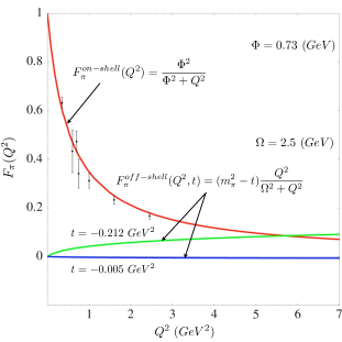
Figure 1: On-shell and off-shell pion form factors. The red line shows the monopole fit of the on-shell formfactor to CHPT results. Experimental data are taken from Amend ; Acker ; Brauel ; Hub . The off-shell form factor is shown for both low ($t=-0.005\,\mbox{GeV}^{2}$, blue line) and high ($t=-0.212\,\mbox{GeV}^{2}$, green line) hadronic momentum transfers.

From Fig.1, one can see that our fit is in rather good agreement with experimental data. We now use the fitted form factors in the calculations of the two-photon box pion electroproduction correction with the same tools for the exact calculations as in AAB2 , for high ($Q^{2}=6.0\,\mbox{GeV}^{2}$) and low ($Q^{2}=0.3\,\mbox{GeV}^{2}$) momentum transfers (see Fig.2).

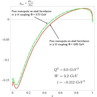
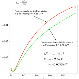
Figure 2: Two-photon box radiative correction for the exclusive pion electroproduction for $Q^{2}=6.0\,\mbox{GeV}^{2}$ (left plot) and $Q^{2}=0.3\,\mbox{GeV}^{2}$ (right plot). The corrections calculated with the monopole pion form factor for $\Phi=0.73\,\mbox{GeV}$ and $\Phi=0.85\,\mbox{GeV}$ are shown by the dashed green and solid red lines, respectively.

Two lines, $\Phi=0.73\,\mbox{GeV}$ (green dashed line) and $\Phi=0.85\,\mbox{GeV}$ (red solid line), illustrate the box correction sensitivity to the choice of the scale in the form factor. As can be clearly seen from the right plot of Fig.2, for the low momentum transfer the correction is rather sensitive to the scale, which induces an additional theoretical uncertainty due to the box correction model dependence. For the high momentum transfer (left plot of Fig.2, we observe that the correction does not change much with the change of the scale in the form factor. Thus, we observe a reduced degree of model dependence in the correction for high momentum transfers. For the off-shell part of the pion form factor, we have observed a contribution of less than 1% to the correction, which certainly diminishes any role of the off-shell form factor in the pion electroproduction process.

III Dynamical Polarizabilities of Mesons

Experimentally, a unique opportunity to study the dynamical structure of hadrons over a wide kinematic range is provided by Compton scattering. In the non-relativistic approximation, the Hamiltonian related to the meson internal structure can be represented as

$$H_{eff}=-\frac{1}{2}4\pi\alpha_{E}\vec{E}^{2}-\frac{1}{2}4\pi\beta_{M}\vec{H}^{2},$$ (6)

where $\alpha_{E}$ and $\beta_{M}$ are electric and magnetic polarizabilities of the meson, respectively. Up to now, only charged and neutral pion polarizabilities have been measured, producing a broad range of values Ahrens ; Antipov ; Ba92 . Precision measurements of the charged pion polarizability through the Primakoff two-pion photo-production process with linearly polarized photons is planned at JLab. The cross section for this process,

$$\frac{d^{2}\sigma}{d\Omega_{\pi\pi}dW_{\pi\pi}}=\frac{2\alpha_{f}Z^{2}}{\pi^{2}}\frac{E_{\gamma}^{4}\beta^{2}}{W_{\pi\pi}}\frac{\sin\theta_{\pi\pi}^{2}}{Q^{4}}|F(Q^{2})|^{2}$$

$$\sigma(\gamma\gamma\rightarrow\pi\pi)(1+2P_{\gamma}\cos 2\phi_{\pi\pi}),$$ (7)

is related to the photon fusion cross section, $\sigma(\gamma\gamma\rightarrow\pi\pi)$, which can be easily turned into a Compton cross section by means of crossing symmetry. In Eq.(7), $W_{\pi\pi}$ is the $\pi\pi$ invariant mass, Z is the atomic number, $E_{\gamma}$ is the energy of the incident photon, $F(Q)$ is the electromagnetic form factor for the proton target, $\theta_{\pi\pi}$ is the lab angle for the two pions, $P_{\gamma}$ is the incident photon polarization and $\phi_{\pi\pi}$ is the azimuthal angle of the $\pi\pi$ system. One can relate photon fusion cross section, $\sigma(\gamma\gamma\rightarrow\pi\pi)$, to the polarizabilities of the pion Ba92 ; Do93 as

$$\sigma_{\gamma\gamma\rightarrow\pi\pi}(|\cos\theta|<Z)=\frac{\kappa}{256\pi s^{2}}\int_{t_{a}}^{t_{b}}dt$$

$$\Bigg{(}\bigg{|}m_{\pi}^{2}B_{o}-8\pi sm_{\pi}\beta+\frac{4\pi}{m_{\pi}}(\alpha+\beta)st\bigg{|}^{2}+$$

$$\bigg{|}B_{o}+\frac{4\pi s}{m_{\pi}}(\alpha+\beta)\bigg{|}^{2}\frac{(m_{\pi}^{4}-tu)^{2}}{s^{2}}\Bigg{)},$$ (8)

where

$$\displaystyle{B_{o}=16\pi\alpha_{f}{\displaystyle\frac{s}{(t-m_{\pi}^{2})(u-m_{\pi}^{2})}}|q|},$$

and

$$\displaystyle t_{b,a}=m_{\pi}^{2}-\frac{1}{2}s\pm\frac{sZ}{2}\beta(s).$$

Here, $s,\,t$ and $u$ are the Mandelstam variables, $|q|$ is the meson charge, $\beta(s)=\sqrt{\frac{s-4m_{\pi}^{2}}{s}}$ is the center-of-mass velocity of produced pions and $\kappa=1$ or $2$ for a neutral or charged pion, respectively. Eqs.7 and III are valid for any meson, not just pions. For real Compton scattering, we can construct an invariant amplitude,

$$\ M(\gamma\pi\rightarrow\gamma^{\prime}\pi)=\epsilon^{\prime\mu}\epsilon^{\nu}\ M_{\mu\nu}.$$ (9)

Here $\boldsymbol{\epsilon}\>\mbox{and }\boldsymbol{\epsilon^{\prime}}$ are polarization vectors of incoming and outgoing photons, respectively, and $M_{\mu\nu}$ is the Compton tensor, which is related to two Compton structure functions ($A(s,t)$ and $B(s,t)$) in the following way:

$$M_{\mu\nu}=A(s,t)\ T_{\mu\nu}^{(1)}+B(s,t)\ T_{\mu\nu}^{(2)}.$$ (10)

The Lorentz tensors, $T_{\mu\nu}^{(1)}$ and $T_{{}_{\mu\nu}}^{(2)}$, are

$$T_{\mu\nu}^{(1)}=-\displaystyle{\frac{t}{2}g_{\mu\nu}-k_{3,\mu}k_{1,\nu}}$$

$$T_{\mu\nu}^{(2)} =\displaystyle{\frac{1}{2t}(s-m_{\pi}^{2})(u-m_{\pi}^{2})g_{\mu\nu}+k_{2,\mu}k_{2,\nu}+}$$ (11)

$$\displaystyle{\frac{s-m_{\pi}^{2}}{t}k_{3,\mu}k_{3,\nu}-\frac{u-m_{\pi}^{2}}{t}k_{2,\mu}k_{1,\nu}}.$$

The amplitude related to the meson electric and magnetic polarizabilities can now be rewritten as

$$\ M(\gamma\pi\rightarrow\gamma^{\prime}\pi)=\alpha\omega^{2}(\boldsymbol{\epsilon}{}^{\prime*}\cdot\boldsymbol{\epsilon})+\beta\omega^{2}({\bf s}{}^{\prime*}\cdot{\bf s}),$$ (12)

where $\omega$ is the photon energy and $\boldsymbol{s}=(\boldsymbol{k}\times\boldsymbol{\epsilon})$ denotes the magnetic vector. Combining Eq.(10) and (12), we get a connection between the polarizabilities and Compton structure functions:

$$\alpha(s,t)=-\frac{1}{8\pi m}\bigg{(}A(s,t)+\frac{s-3m^{2}}{t}B(s,t)\bigg{)}$$

(13)

$$\beta(s,t)=\frac{1}{8\pi m}\bigg{(}A(s,t)+\frac{s-m^{2}}{t}B(s,t)\bigg{)}.$$

Terms in Eq.(13) are clearly energy-dependent, so we call them dynamical. In the limit when $s\rightarrow m^{2}$ and $t\rightarrow 0$, we recover the static values of the polarizabilities. Using CHM and restricting our calculations to one-loop in CHPT (two-loop SU(2) calculations were done in Ga06 and showed a rather small impact on the cross section in Primakoff reaction), we calculate the dynamical polarizabilities of mesons including the entire SU(3) octet of mesons in the loop integrals.

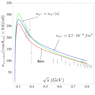
Figure 3: Left graph: energy dependence of the pion electric polarizabilty. Right graph: $\gamma\gamma\rightarrow\pi\pi$ cross section, where red line corresponds to the Born cross section, blue line is the cross section related to the static CHPT value of polarizability and green line shows the cross section with dynamical polarizabilities from Eq.(13). The data points are taken from MARK-II Bo92 .

In addition, we include a structure-dependent pole contribution arising from the vector mesons in similar fashion to Ba92 ; Do93 . We now have the following static electric and magnetic polarizabilities (in units of $10^{-4}\mbox{fm}^{3}$):

$$\alpha_{\pi^{\pm}}=\frac{8\alpha_{f}}{m_{\pi}f_{\pi}^{2}}(L_{9}+L_{10})=2.83;$$

$$\beta_{\pi^{\pm}}=-\alpha_{\pi^{\pm}}+\frac{m_{\pi}}{4\pi}\frac{G_{\rho}}{M_{\rho}^{2}-m_{\pi}^{2}}=-2.76$$

$$\alpha_{\pi^{0}}=-\frac{\alpha_{f}}{48\pi^{2}m_{\pi}f_{\pi}^{2}}=-0.50;$$

$$\beta_{\pi^{o}}=-\alpha_{\pi^{o}}+\frac{m_{\pi}}{4\pi}\sum_{V=\rho,\omega}\frac{G_{V}}{M_{V}^{2}-m_{\pi}^{2}}=1.25.$$ (14)

The pion coupling constant is $f_{\pi}=\sqrt{2}F_{\pi}=130.7\,\mbox{MeV}$, $\alpha_{f}$ is the fine structure constant, the low energy constants are $L_{9}=(5.99\pm 0.43)\cdot 10^{-3}$ and $L_{10}=(-4.5\pm 0.7)\cdot 10^{-3}$, and for the vector mesons coupling constants we use $G_{\rho}=0.044\,\mbox{GeV}$ and $G_{\omega}=0.495\,\mbox{GeV}$. The polarizabilities for the octet of mesons are summarized in Table 1.

($10^{-4}\,\mbox{fm}^{3}$)	$\alpha-\beta$	$\alpha+\beta$
$\pi^{\pm}$	5.59	0.07
$\pi^{0}$	-1.75	0.75
$\eta$	-0.044	0.0
$K^{\pm}$	0.88	0.0
$K^{0}$	0.0032	0.0

Table 1: Meson electric and magnetic static polarizabilities

To extract the static pion polarizabilities from the $\gamma\gamma\rightarrow\pi\pi$ cross section, one can use Eq.(13) (with crossing symmetry $s\rightarrow t$ and $t\rightarrow s$) substituted into Eq.(III). The important role of the energy dependence of the polarizabilities in the description of the $\gamma\gamma\rightarrow\pi\pi$ cross section can be seen in Fig.3. In Fig.4, it is clearly visible that the dynamical polarizability of the kaon has a very strong influence on the $\gamma\gamma\rightarrow K^{+}K^{-}$ cross section.

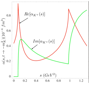
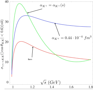
Figure 4: Charged kaon dynamical polarizability and prediction for the $\gamma\gamma\rightarrow K^{+}K^{-}$ cross section. On the left plot, red line is the Born cross section, blue line corresponds to the static polarizability and green line to the dynamical polarizability cross section.

IV Dynamical Polarizabilities of Baryons

The electric and magnetic polarizabilities of baryons introduce an additional contribution into the effective Hamiltonian for baryons in the electromagnetic field in the same way as defined in Eq.(6). The current PDG PDG experimental values for the electric and magnetic polarizabilities for proton and neutron are (in units of $10^{-4}\mbox{fm}^{3}$):

$$\alpha_{p}=12.0\pm 0.6; \beta_{p}=1.9\pm 0.5;$$

$$\alpha_{n}=11.6\pm 1.5; \beta_{n}=3.7\pm 2.0.$$

In order to evaluate polarizabilities theoretically, one can use Compton scattering and relate an amplitude to the set of Compton structure functions $R_{i}$ Babusci in the following way:

$$\displaystyle{\frac{1}{8\pi W}}M(\gamma B\rightarrow\gamma^{\prime}B)=R_{1}(\boldsymbol{\epsilon}{}^{\prime*}\cdot\boldsymbol{\epsilon})+R_{2}({\bf s}{}^{\prime*}\cdot{\bf s})+$$

$$iR_{3}\boldsymbol{\sigma}\cdot(\boldsymbol{\epsilon}{}^{\prime*}\times\boldsymbol{\epsilon})+iR_{4}\boldsymbol{\sigma}\cdot({\bf s}{}^{\prime*}\times{\bf s})+$$

$$iR_{5}((\boldsymbol{\sigma}\cdot\hat{{\bf k}})({\bf s^{\prime*}}\cdot\boldsymbol{\epsilon})-(\boldsymbol{\sigma}\cdot\hat{{\bf k}}^{\prime})({\bf s}\cdot\boldsymbol{\epsilon^{\prime*}}))+$$

$$iR_{6}((\boldsymbol{\sigma}\cdot\hat{{\bf k}}^{\prime})({\bf{\bf s^{\prime*}}}\cdot\boldsymbol{\epsilon})-(\boldsymbol{\sigma}\cdot\hat{{\bf k}})({\bf s}\cdot\boldsymbol{\epsilon^{\prime*}})).$$ (15)

Here, $W=\omega+\sqrt{\omega^{2}+m_{B}^{2}}$ is the center of mass energy and $\omega$ is the energy of the incoming photon. The unit magnetic vector (${\bf s}=(\hat{{\bf k}}\times\boldsymbol{\epsilon}$)), the polarization vector ($\boldsymbol{\epsilon}$) and the unit momentum of the photon (${\displaystyle\hat{{\bf k}}=\frac{{\bf k}}{k}}$) are denoted with a prime in the case of the outgoing photon. Although the choice of the basis for the invariant Compton amplitude is not unique and can be defined differently Babusci , the basis in Eq.(15) is more convenient for the evaluation of the polarizabilities because in this basis the structure functions, $R_{i}$, are directly related to the electric, magnetic and spin-dependent polarizabilities in the multipole expansion.

It is well known that parameters such as polarizabilities can be determined by the non-Born contributions to the Compton structure functions. This includes loops (up to the given order of perturbation) and structure-dependent pole contributions, such as tree-level baryon resonance excitations and the WZW anomalous interaction (contributing only into backward spin-dependent polarizability). If in the multipole expansion of the Compton structure functions multi-1 ; multi-2 ; multi-3 we keep only the dipole-dipole and dipole-quadrupole transitions, we can obtain simple equations connecting non-Born (NB) structure functions to the polarizabilities of the baryon:

$$R_{1}^{NB}=\omega^{2}\alpha_{E1};\ \ R_{2}^{NB}=\omega^{2}\beta_{M1};$$

$$R_{3}^{NB}=\omega^{3}(-\gamma_{E1E1}+\gamma_{E1M2});$$

$$R_{4}^{NB}=\omega^{3}(-\gamma_{M1M1}+\gamma_{M1E2});$$

$$R_{5}^{NB}=-\omega^{3}\gamma_{M1E2};\ \ R_{5}^{NB}=-\omega^{3}\gamma_{E1M2}.$$ (16)

Although the polarizabilities used in the Eq.(16) are defined as constants, it is essential to treat them as energy-dependent quantities Griesshammer because the Compton scattering experiments were performed with 50 to 800 MeV photons and hence require additional theoretical information to extrapolate the results to zero-energy parameters. The polarizabilities become energy-dependent due to the internal relaxation mechanisms, resonances, and particle production thresholds. Accordingly, if for the static polarizabilities we only keep order up to $\mathcal{O}(\omega^{2})$ for $R_{1,2}$ and up to $\mathcal{O}(\omega^{3})$ for $R_{3,4,5,6}$ then for energy-dependent dynamical polarizabilities we keep all orders in $\omega$ in the Compton structure functions. The calculation of the Compton structure functions up to the one-loop order in the framework of relativistic CHPT was made possible by CHM CHM . In addition, the structure-dependent pole contribution to the nucleon polarizabilities has been taken into account in the form of the nucleon $\Delta$-resonance excitation. A Lagrangian which describes nucleon-to-resonance radiative transition is given in the form of a contact term:

$$\displaystyle{\mathcal{L}^{\Delta N\gamma}=i\Theta\frac{e}{\Lambda}\bar{N}\gamma^{\mu}\gamma_{5}Q\Delta^{\nu}F_{\mu\nu},}$$

(17)

$$F_{\mu\nu}=\partial_{\mu}\mathcal{A}_{\nu}-\partial_{\nu}\mathcal{A}_{\mu}.$$

Here, $\Lambda\sim 1\,GeV$ is the scale of chiral symmetry breaking and $\Theta$ is the coupling strength, determined from the branching ratio of the radiative decay, $\Delta\rightarrow N\gamma$. The $\Delta$ resonance propagator is described by the propagator of the 3/2 spin Rarita-Schwinger field:

$$\Pi_{\Delta}^{\mu\nu}=\frac{1}{2m}\frac{\not p+m}{p^{2}-m^{2}+im\Gamma}\Big{(}g^{\mu\nu}-\frac{1}{3}\gamma^{\mu}\gamma^{\nu}-$$

$$\frac{2p^{\mu}p^{\nu}}{3m^{2}}+\frac{p^{\mu}\gamma^{\nu}-p^{\nu}\gamma^{\mu}}{3m}\Big{)}.$$ (18)

The polarizabilities calculated for the proton with the photon energies up to 300 MeV are shown in Fig.5. It is evident that below 50 MeV these polarizabilities have small energy dependence. For the neutron, the energy dependencies of dynamical polarizabilities have very similar behavior except the values are bigger on the absolute scale, so we will only describe the dynamical polarizabilities for the proton.

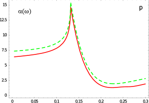
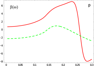
Figure 5: Dependencies of the proton electric and magnetic polarizabilities (in $10^{-4}\,(fm^{3})$) on photon energy, $\omega$ (GeV), in the center-of-mass reference frame. Green-dashed curves correspond to the meson-nucleon loops contribution only; solid-red curves include the $\Delta$-resonance pole contribution.

The electric polarizability of the proton has very strong resonance type dependence near the pion production threshold. The $\Delta$-pole contribution has a small effect while consistently reducing $\alpha_{p}(\omega)$ values for all energies. Of course, to make final predictions for the CHPT values of polarizabilities, we need to add the contribution from the resonances in the loops of Compton scattering. Hence, in order to compare our results with the experimental values, we have borrowed the resonance loops results from the small-scale expansion (SSE) approach SSE . If no $\Delta$-pole contribution is added, the magnetic polarizability in Fig.5 stays negative (diamagnetic) for almost all the energies. The $\Delta$-pole contribution is very big and shifts $\beta_{p}(\omega)$ from negative to positive (paramagnetic) values for energies up to 250 MeV. This behavior is quite natural since the pion loop calculations reflect magnetic polarizability coming from the virtual diamagnetic pion cloud and the $\Delta$ resonance contribution to $\beta_{p}(\omega)$ is driven by the strong paramagnetic core of the nucleon. Our results for the proton polarizabilities calculated in relativistic CHPT up to one-loop order including the $\Delta$- pole and SSE contribution are the following (in units of $10^{-4}(fm^{3}))$:

$$\alpha_{p}=(7.38\,(\pi-\mbox{loop})-0.95\,(\Delta-\mbox{pole})+$$

$$4.2\,(\mbox{SSE}))=10.63;$$

$$\beta_{p}=(-2.20\,(\pi-\mbox{loop})+3.0\,(\Delta-\mbox{pole})+$$

$$0.7\,(\mbox{SSE}))=1.49.$$

The static electric and magnetic polarizabilities for hyperons have been calculated first in Meissner in the heavy baryon chiral perturbation theory. The dynamical electric and magnetic polarizabilities for hyperons were first calculated in AB . In Fig.6, we provide our results for dynamical electric and magnetic polarizabilities for hyperons using the basis from Eq.(15) in the Compton scattering amplitude.

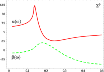
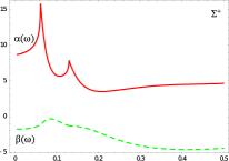
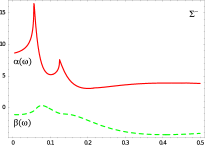
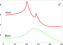
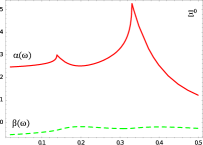
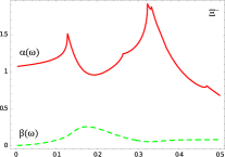
Figure 6: Electric and magnetic dynamical polarizabilities of hyperons in units of $10^{-4}\,(fm^{3})$ as a function of the photon energy, $\omega$ (GeV). Here, the solid-red line represents the electric polarizability, and the dashed-green line is the magnetic polarizability.

For all polarizabilities listed in Fig.(6), the electric polarizabilities have very similar resonant-type behavior near meson-production thresholds and the magnetic polarizabilities for all hyperons have negative low energy (static) values. Once again, it is important to include both pole and loop resonance contributions for a complete analysis. It is clear that for the all dynamical polarizabilities of the SU(3) octet of baryons, the values are strongly governed by the excitation mechanism reflected in the meson production peaks. Hence, the study of these polarizabilities directly probes the internal degrees of freedom governing the baryon structure at low energies.

V Conclusions

In this work, we have evaluated the pion form factor and have investigated its influence on the behavior of the two-photon box pion electroproduction correction. We also calculated the dynamical polarizabilities of mesons including the entire SU(3) octet of mesons in the loop integrals using relativistic CHPT implemented in CHM. The dynamical electric and magnetic polarizabilities of the SU(3) octet of baryons were investigated in detail. We found that predictions of the chiral theory derived from our calculations (up to one-loop order and not including resonances in loop calculations) are somewhat consistent with the experimental results. The dependencies for the range of photon energies covering the majority of the meson photo production channels were analyzed. These extensive calculations are made possible by the recent implementation of semi-automatized calculations in CHPT, which allows the evaluation of polarizabilities from Compton scattering up to next-to-the-leading order. Our current goal is the calculation of dynamical polarizabilities with baryon resonances in the loops. There is still some disagreement between heavy-baryon and relativistic versions of CHPT introducing theoretical uncertainty. Clearly, further experimental work is needed especially for the hyperon and strange mesons polarizabilities, which would help with the further development of the theory.

VI Acknowledgements

This work has been supported by the Natural Sciences and Engineering Research Council of Canada (NSERC).

References

- (1) J. Gasser and H. Leutwyler, Ann. Phys. 158, 142 (1984).
- (2) V. A. Nesterenko and A. V. Radyushkin, Phys. Lett. B115 410 (1982); A.V. Radyushkin, Nucl. Phys. A532 141 (1991).
- (3) R. Jakob and P. Kroll, Phys. Lett. B315 463 (1993).
- (4) F. Cardarelli et al., Phys. Lett. B332 (1994) 1; Phys. Lett. B357 267 (1995).
- (5) H. Ito, W. W. Buck and F. Gross, Phys. Rev. C 45 (1992) (1918).
- (6) P. Maris and P. C. Tandy, preprint nucl-th/0005015.
- (7) V. Tadevosyan et al., Phys. Rev. C 75, 055205 (2007); T. Horn et al., Phys. Rev. Lett. 97, 192001 (2006).
- (8) N. Dombey, Rev. Mod. Phys. 41, 236 (1969).
- (9) A. Afanasev, A. Akushevich, Burkert, Joo, Phys.Rev.D66: 074004 (2002).
- (10) A. Afanasev, A. Aleksejevs and S. Barkanova, preprint arXiv:1207.1767.
- (11) A. Aleksejevs, M. Butler, J.Phys.G37,035002 (2010).
- (12) S. R. Amendolia et al., Nucl. Phys. B277, 168 (1986); S. R. Amendolia et al., Phys. Lett. B146, 116 (1984).
- (13) H. Ackermann et al., Nucl. Phys. B137, 294 (1978).
- (14) P. Brauel et al., Z. Phys. C 3, 101 (1979).
- (15) G. M. Huber et al., Phys. Rev. C 78, 045203 (2008).
- (16) J. Ahrens et al., Eur. Phys. J. A23, 113 (2005).
- (17) Yu. M. Antipov et al., Phys. Lett. B121, 445 (1983).
- (18) D. Babusci, et al. Phys. Lett. B 277, 158 (1992).
- (19) J. F. Donoghue and B. R. Holstein, Phys. Rev. D 48, 137 (1993).
- (20) J. Gasser, M.A. Ivanov, and M. E. Sainio, Nucl. Phys. B745, 84 (2006).
- (21) J. Boyer et al. (MARK-II collaboration), Phys. rev. D 42, 1350 (1990).
- (22) J. Beringer et al. (Particle Data Group), Phys. Rev. D86, 010001 (2012).
- (23) B. Pasquini, D. Drechsel, and M. Vanderhaeghen, Eur. Phys. J. Special Topics 198, 269–285 (2011).
- (24) D. Babusci, G. Giordano, A.I. L’vov , G. Matone, A.M. Nathan, Phys.Rev. C58 (1998) 1013-1041
- (25) R. P. Hildebrandt, H. W. Griesshammer, T. R. Hemmert, B. Pasquini, Eur. Phys. J A 20, 293-315 (2004).
- (26) T. R. Hemmert, B. R. Holstein, J. Kambor, Phys. Rev. D 55, 5598 (1997).
- (27) V.I. Ritus, ZhETP 32, 1536 (1957) [Sov. Phys. JETP 5, 1249 (1957)].
- (28) [53] A.P. Contogouris, Nuovo Cim. 25, 104 (1962).
- (29) Y. Nagashima, Progr. Theor. Phys. 33, 828 (1965).
- (30) Lensky & Pascalutsa Eur.Phys.J.C65:195-209, (2010).
- (31) T. R. Hemmert, B. R. Holstein, J. Kambor and G. Knochlein, Phys. Rev. D 57, (1998) 5746.
- (32) K. B. Vijaya Kumar, J. A. McGovern and M. C. Birse, Phys. Lett. B 479, (2000) 167.
- (33) G. C. Gellas, T. R. Hemmert and U. G. Meissner, Phys. Rev. Lett. 86, (2001) 3205.
- (34) D. Drechsel, B. Pasquini and M. Vanderhaeghen, Phys. Rept. 378, (2003) 99.
- (35) V. Bernard, N. Kaiser, J. Kambor and U. Meissner, Phys. Rev. D 46, 7 (1992).
- (36) K.B. Kumar, A. Faessler, T. Gutsche, B. Holstein, V. Lyubovitskij, Phys.Rev. D84, 076007 (2011).
- (37) A. Aleksejevs and S. Barkanova, J.Phys. G38 (2011) 035004