A non-linear mathematical model of cell turnover, differentiation and tumorigenesis in the intestinal crypt.

Abstract

We present a development of a model of the relationship between cells in three compartments of the intestinal crypt: stem cells, semi-differentiated cells and fully differentiated cells. Stem and semi-differentiated cells may divide to self-renew, undergo programmed death or progress to semi-differentiated and fully differentiated cells respectively. The probabilities of each of these events provide the most important parameters of the model. Fully differentiated cells do not divide, but a proportion undergoes programmed death in each generation. Our previous models showed that failure of programmed death - for example, in tumorigenesis - could lead either to exponential growth in cell numbers or to growth to some plateau. Our new models incorporate plausible fluctuation in the parameters of the model and introduce non-linearity by assuming that the parameters depend on the numbers of cells in each state of differentiation. We present detailed analysis of the equilibrium conditions for various forms of these models and, where appropriate, simulate the changes in cell numbers. We find that the model is characterized by bifurcation between increase in cell numbers to stable equilibrium or ’explosive’ exponential growth; in a restricted number of cases, there may be multiple stable equilibria. Fluctuation in cell numbers undergoing programmed death, for example caused by tissue damage, generally makes exponential growth more likely, as long as the size of the fluctuation exceeds a certain critical value for a sufficiently long period of time. In most cases, once exponential growth has started, this process is irreversible. In some circumstances, exponential growth is preceded by a long plateau phase, of variable duration, mimicking equilibrium: thus apparently self-limiting lesions may not be so in practice and the duration of growth of a tumor may be impossible to predict on the basis of its size.

¹ Division of Epidemiology and Biostatistics, European Institute of Oncology, Via Ripamonti 435, Milano, Italy, I-20141
EMAIL: alberto.donofrio@ieo.eu
² Molecular and Population Genetics Laboratory, Cancer Research UK, 44, Lincoln’s Inn Fields, London WC2A 3PX. UK

Keywords: Tumorigenesis – Apoptosis – Nonlinearity – Bifurcations – Random – Cellualr communication

1 Introduction

The crypt of the large intestine is a widely used model for studying the division of stem cells, for observing the differentiation and, ultimately, death of cells arising from those stem cells, and for the genesis of tumors resulting from abnormalities of cell division and/or death and/or migration. We have previously set up simple models of cell birth, differentiation and death in the colonic crypt and used these to analyze parameters of cell behavior which led to stable equilibria and to tumorigenesis if those parameters were altered. Our results showed that the classical exponential growth of an expanding tumor clone could occur, but that mutations with weaker effects, particularly on programmed cell death (PCD), could cause tumor growth to a new equilibrium or plateau level of cells. We speculated that such a form of tumor growth might be particularly applicable to benign lesions which rarely progress to malignancy, such as hyperplastic polyps of the colorectum, or lipomas of the skin.

The model which we originally described was based on a commonly used simplification of the cell populations within the colonic crypt (see table 1 of [1]). A population of stem cells (number $x_{G}$ at generation $G$) was assumed to replicate at a specified rate (division time $t_{o}$). Each stem cell underwent PCD with probability $\alpha_{1}$, renewed itself with probability $\alpha_{3}$ , or progressed to a state of semi-differentiation ($p=\alpha_{2}$). Usually, $x_{G}$ was assumed to be constant, with $\alpha_{3}$ set to 0.5. For the population of semi-differentiated cells (the size of which at generation $G$-th will be indicated as $y_{G}$ ), division could lead to PCD, renewal or progression to a fully differentiated state (the size of which at generation $G$-th will be indicated as $Z_{G}$). Fully differentiated cells underwent PCD with a probability $\gamma$. Mathematically, following the above assumptions, the dynamics of the cell population was ruled by the linear equations:

$$x_{G+1} = 2\alpha_{3}x_{G}$$

$$y_{G+1} = 2\beta_{3}\frac{t_{o}}{t_{1}}y_{G}+2\alpha_{2}x_{G}$$ (1)

$$z_{G+1} = 2\beta_{2}\frac{t_{o}}{t_{1}}y_{G}+(1-\gamma\frac{t_{o}}{t_{2}})z_{G}$$

where, of course: $\alpha_{1}+\alpha_{2}+\alpha_{3}=1$ and $\beta_{1}+\beta_{2}+\beta_{3}=1$. If we assume that $x_{G}$ is constant, it has to be that $\alpha_{3}=0.5$ and the first equation reads $x_{G+1}=x_{G}$. When $2\beta_{3}\frac{t_{o}}{t_{1}}<1$ the number of semi-differentiated cells evolves to the following equilibrium value $y_{eq}=(2\alpha_{2}x_{G})/(1-2\beta_{3}\frac{t_{o}}{t_{1}})$, with $y_{eq}$ proportional to $x_{G}$. Instead when $2\beta_{3}\frac{t_{o}}{t_{1}}\geq 1$ there is an exponential increase $y_{G}\rightarrow+\infty$ as $G\rightarrow+\infty$. Therefore, $\beta_{3}$ is a bifurcation parameter [4, 7], that is, there exists a critical value

$$K=\frac{t_{1}}{2t_{o}}$$

such that the behavior of the system for $\beta_{3}<K$ (that is, $y_{G}\rightarrow y_{eq}$) is not equivalent to the behavior for $\beta_{3}\geq K$ ( $y_{G}\rightarrow+\infty$). Clearly, $\alpha_{3}$ is also a bifurcation parameter. Note, however, that if $\alpha_{3}=0.5$, the constant number of stem cells and the rate of progression to a semi-differentiated state are not bifurcation parameters. If they have a small variations, the behavior of $y_{G}$ does not change qualitatively and has only a small numerical variation.

In this manuscript, we extend our model to include situations in which there is random fluctuation in cell numbers within each compartment and to situations in which the probabilities of PCD, differentiation or renewal depend on the number of cells in each compartment. Incorporating these assumptions introduces non-linearity into the model, with consequences for the maintenance of stable equilibria within the crypt cell populations.

2 Non-linear extension of the model

Let us assume that some function of the number of semi-differentiated cells may increase or reduce the probability of PCD. In the former case, the system has, as in the linear model, only one global asymptotic equilibrium $y_{eq}$. As a consequence, the parameter $2(t_{o}/t_{1})\beta_{3}(y)$ is a decreasing function of $y$, and it may be seen that $y_{eq}$ is smaller than the value $2\alpha_{2}/X(1-2\beta_{3}(t_{o}/t_{1}))$ which would be reached if $\beta_{3}$ were constant. This situation may represent normal homeostasis. In contrast, let us consider the latter case, which represents an abnormal situation, perhaps one which results from mutation in the stem cell compartment. In the latter case, we shall allow $\beta_{1}(y)$ to be a decreasing function of $y$, whereas we will consider , $\beta_{2}(y)$ constant or slowly growing, so that $\beta_{3}(y)$ is a growing function of the number of semi-differentiated cells. Furthermore we consider that for low $y$ the variation of that function is slow, such that it initially is approximately constant. Because of their nature $\beta_{1},\beta_{2},\beta_{3}\in(0,1)$ and therefore these parameters shall have asymptotic values, as in figure 1. In practice the $\beta$ functions model a sort of loose threshold mechanism. We do not place a particular constraint on the analytical form of these functions, since the results which we shall present are qualitatively dependent only on the ”shape” of $\beta_{3}(y)$. For the simulations which we shall propose we shall use :

$$\beta_{3}(y)=\beta_{3_{min}}+0.5\beta_{3_{Max}}\Big{(}1+\frac{2}{\pi}Atan\big{(}A(y-y_{m})\big{)}\Big{)},A>>1$$

or

$$\beta_{3}(y)=\begin{cases}\beta_{3_{min}}&\text{if $y<y_{1}$ },\\ \beta_{3_{min}}+\frac{\beta_{3_{Max}}-\beta_{3_{min}}}{y_{2}-y_{1}}(y-y_{1})&\text{if $y_{1}\leq y\leq y_{2}$ },\\ \beta_{3_{Max}}&\text{if $y<y_{1}$ }.\end{cases}$$

Thus instead of the linear set of equations (1) we have the following nonlinear discrete dynamical system:

$$x_{G+1} = 2\alpha_{3}x_{G}$$

$$y_{G+1} = 2\frac{t_{o}}{t_{1}}\beta_{3}(y_{G})y_{G}+2\alpha_{2}x_{G}$$ (2)

$$z_{G+1} = 2\frac{t_{o}}{t_{1}}\beta_{2}(y_{G})y_{G}+(1-\gamma\frac{t_{o}}{t_{2}})z_{G}$$

Note that the behavior of $z_{G}$, being $0<(1-\gamma\frac{t_{o}}{t_{2}})<1$, is determined by the behavior of $y_{G}$:

• When $y_{G}\rightarrow+\infty$ also $z_{G}\rightarrow+\infty$;

• when $y_{G}\rightarrow+y_{eq}$ also $z$ tends to an equilibrium point.

Therefore, in the next section, we shall deal only with the dynamics of $x_{G}$ and $y_{G}$.

3 Non-linear model: fluctuation in the number of semi-differentiated cells depends on stem cell number and on $\alpha_{2}$

In this section we shall set

$$U=2\alpha_{2}x_{G}$$

and consider it as a static parameter in the input to the equation for the semi-differentiated cells. The equilibrium equation reads

$$y=2\beta_{3}(y)(t_{o}/t_{1})y+U$$

which we shall rearrange in the more convenient form:

$$2\beta_{3}(y)(t_{o}/t_{1})=1-\frac{U}{y}$$ (3)

that is, the equilibrium is determined by the intersection of the $2\beta_{3}(y)(t_{o}/t_{1})$ curve with the family of hyperbolae $1-(U/y)$. The dynamics of the model are essentially determined by the asymptotic value $2\beta_{3}(+\infty)(t_{o}/t_{1})$.

3.1 Excess self-renewal of semi-differentiated cells

Here

$$2\beta_{3}(+\infty)(t_{o}/t_{1})>1.$$

As a consequence, there exists (see Figure 2) a threshold value $U_{m}$ for $U$, such that for each $U\in(0,U_{m})$ there are two points of intersection, (that is, two equilibria); for $U=U_{m}$, the lines collide, and for $U>U_{m}$ there are no equilibrium points. In the limit case $U=U_{m}$ there is tangency (a double equilibrium point). The higher the value of $U$, the more to the right are the hyperbolae. From a static point of view (that is, considering different but constant values of $U$), there is a saddle node bifurcation [4, 7]. From figure 3-(a) , we see that for $U<U_{m}$, there is a stable lower equilibrium $y^{Stab}(U)$, followed by an unstable equilibrium $y^{Unst}(U)$; the equilibria tend to collide for $U\rightarrow U_{m}$. The point $y^{Stab}(U)$ has an attraction basin equal to the whole range $\big{(}0,y^{Unst}(U)\big{)}$, which is easily verified by using the following Liapunov-La Salle function $L(y)=|y-y^{Stab}(U)|$. For all $y\in(y^{Unst}(U),+\infty)$, there is instability and unbounded growth of the number of semi-differentiated cells ($y\rightarrow+\infty$). From figure 3, the critical threshold value corresponds to the maximum of the curve $U=U(Y_{eq})$ $=$ $Y_{eq}(1-2(t0/t1)\beta_{3}(Y_{eq}))$. As a consequence $U_{m}=Y_{m}(1-2(t0/t1)\beta_{3}(Y_{m}))$ where $Y_{m}$ is the unique real solution of the null derivative equation $\frac{dU(Y)}{dY}=0\Rightarrow 2\frac{t0}{t1}(\beta_{3}(Y)+\frac{d\beta_{3}(Y)}{dY})=0$ From figures 2 and 3-(a), it is evident that the first, stable equilibrium point is proportional to $U$ for small and also ”moderately small” values of this parameter, since the first intersection between the hyperbola $1-U/y$ and the curve $2(t0/t1)\beta_{3}(Y)$ is located in the a zone in which the second curve is approximately constant. Let us simulate what happens in the proximity of the bifurcation value $U_{m}$. Figure 3-(b) shows a simulation of a system having $U$ slightly lower than $U_{m}$. It shows classical behavior, initial growth followed by a plateau. There is no qualitative difference between this behavior and that shown in figure 2 of [1]. A more interesting situation is shown in figure 3-(c), in which $U$ is slightly greater than $U_{m}$ and in which the plateau is only temporary, since it is followed by an exponential ”explosion”. A small positive variation around $U_{m}$, therefore, makes the system grow without bound.

3.2 Random fluctuation in cell numbers

We have analyzed the bifurcation of the growth in cell numbers from a static point of view, for given values of the parameter $U$, that is, for given values of the number of stem cells and of the rate of progression from stem cell to semi-differentiated cell. In reality, the bifurcation may be driven by dynamic phenomena, such as variation - even if transient - in the number of stem cells. The rate of PCD or the rate of progression to semi-differentiated cells may also vary. We shall simulate such variability by means of the following non-linear, stochastic, discrete dynamic system, using the original model

$$x_{G+1} = 2\alpha_{3}(G)x_{G}$$

$$y_{G+1} = 2\frac{t_{o}}{t_{1}}\beta_{3}(y_{G})y_{G}+2\alpha_{2}(G)x_{G}$$ (4)

$$z_{G+1} = 2\frac{t_{o}}{t_{1}}\beta_{2}(y_{G})y_{G}+(1-\gamma\frac{t_{o}}{t_{2}})z_{G}$$

except that $\alpha_{3}(G)$ and $\alpha_{2}(G)$ are now stochastic processes. First, we simulated a sporadic random increase in the number of stem cells near the bifurcation by considering a constant $\alpha_{2}$ such that

$$\alpha_{2}x_{1}=U_{m}(1-\omega),\omega<<1$$

that is, $U$ is slightly under the bifurcation value. We assume a stochastically varying $\alpha_{3}$, which will follow this rule:

$$\alpha_{3}(G)=\begin{cases}0.5&\text{if $G<G_{1}$ or $G>G_{2}$ },\\ 0.5+\eta&\text{if $G\in[G_{1},G_{2}]$ }.\end{cases}$$

with $G_{1}$,$G_{2}$ and $\eta$ random variables and such that $\alpha_{2}x(G_{2})>U_{m}$ . The result patterns are identical (exponential growth) in each simulation, but with different start-points for the exponential ’explosion’ in growth. Therefore, this model seems to indicate that, since the exponential growth may be due to saddle-node bifurcations (from a steady state to an unbounded growth) and since these phenomena may be driven by a small noise, the initial time in which this growth (for example, that of a tumor) starts is not calculable in a deterministic way. We also undertook different stochastic simulations, in which we assumed that $\alpha_{2}(G)$ , $\alpha_{3}(G)$ are gaussian or uniform random variables with $E[\alpha_{3}(G)]=0.5$. The standard deviation was variable and such that for a finite number of generations $Prob(U_{G}>U_{m})$ is significantly greater than $0$. The mean values of parameters are such that, if the system were deterministic, it would have a plateau (that is, $E[U]<U_{m}$). The simulations showed that all outcomes do not result in exponential ’explosion’ in a given finite temporal window. Intuitively, this means that the random effects do not sufficiently ’scramble’ the system to drive it into the zone of instability. More formally, given the stochastic process $U_{G}=\alpha_{2}(G)x_{G}$, there is exponential growth only if, at the generation $G$ when $U(G)$ assumes its minimum value $\hat{U}$, the number $y(G)$ of semi-differentiated cells is such that $y\in(y^{Unst},+\infty)$. We performed stochastic simulations for various mean values of $U$ such that $E[U]<U_{m}$, constant $\alpha_{2}$ and each $\alpha_{3}(G)$ gaussian with mean 0.5 and $\sigma=0.05$ ( which implies that $E[U]=2\alpha_{2}X_{0}$ ). The simulations showed that also for low values of $E[U]$ there may be exponential ’explosion’ in a fixed number of generations (for ex. 100) and that for $G\rightarrow+\infty$ there is exponential ’explosion’ in all cases.

The possible behaviors with random variations of $U$ can be summarized as follows:

• if $U=U_{1}<U_{m}$ increases in a random generation $G$ to an upper value $U_{2}>U_{m}$, the system loses its equilibrium and exponential growth starts;

• if $U$ varies randomly in a range $[a,b]$, with $b<U_{m}$, there is no loss of equilibrium;

• if $U$ varies randomly for a finite number of generations in a range $[a,b]$, with $b>U_{m}$ , there may or may not be loss of equilibrium;

• if $U$ varies randomly and permanently in a range $[U_{o}-c,U_{o}+c]$, with $c>0$ and $E[U]=U_{o}\geq U_{m}$ , there is loss of equilibrium in the long run;

• if $U$ varies randomly and permanently in a range $[U_{o}-c,U_{o}+c]$, with $c>0$ and $U_{o}<U_{m}$ , we may find an $\epsilon>0$ such that if $c>(U_{m}-U_{o})(1+\epsilon)$ there is loss of equilibrium in the long run, whereas if $c<(U_{m}-U_{o})(1+\epsilon)$, $y_{+\infty}$ remains bounded.

3.3 No excess renewal of semi-differentiated cells

Here:

$$2\beta_{3}(+\infty)(t_{o}/t_{1})<1$$

As a consequence, as shown in figure 4, for increasing values of $U$ the system passes from $EQ1$ to $EQ3$ and back to $EQ1$ equilibrium points. This is a typical situation which leads to a hysteresis bifurcation diagram [4], as in figure 5-(a). It is possible to determine $2$ particular values for $U$, let us call them $U_{\mu}$ and $U_{m}$ with $U_{m}>U_{\mu}$, such that:

• For $U<U_{\mu}$ there is one globally asymptotically stable equilibrium, $y_{low}(U)$;

• For $U>U_{m}$ there is one globally asymptotically stable equilibrium, $y_{high}(U)$;

• For $U_{\mu}<U<U_{m}$ there are three coexisting equilibria: a new third unstable equilibrium $y_{mid}(U)$ (with: $y_{low}(U)<y_{mid}(U)<y_{high}(U)$ ); and the two previous equilibria: $y_{low}(U)$ (with basin of attraction now: $[0,y_{mid}(U))$ ) and $y_{high}(U)$ (with basin of attraction: $(y_{mid}(U),+\infty)$).

The above stated stability properties are easily proved by using these two Liapounov-La Salle functions: $V_{low}(y)=|y-y_{low}(U)|$ and $V_{high}(y)=|y-y_{high}(U)|$.

With reference to the bifurcation diagram, $U_{\mu}$ and $U_{m}$ correspond, respectively, to the minimum and maximum of the bifurcation curve $U=U(Y_{eq})$. In this case, if we call $Y_{\mu}$ and $Y_{M}$ (with $Y_{M}<Y_{\mu}$ ) the two solutions of the equation $dU/dY=0$, we obtain

$$U_{\mu}=Y_{\mu}(1-2(t0/t1)\beta_{3}(Y_{\mu})),U_{m}=Y_{M}(1-2(t0/t1)\beta_{3}(Y_{M})$$

By using the terminology of catastrophe theory, when $U$ varies and become the greater (lower) than the value of $U_{m}$ ($U_{\mu}$), there is an elementary catastrophe, (that is, with an infinitesimal variation of a control parameter, $U$ in our case, there is a finite variation in the equilibrium point). In figure 5, the effect of the hysteresis bifurcation on cell numbers is shown by means of two simulations: in particular in figure 5-(b), corresponding to a value of $U$ slightly greater than $U_{m}$, the system appears to have reached its equilibrium, but restarts, increasing to reach a new and higher asymptotic value.

Furthermore, in the case in which the deterministic model has two, co-existing, alternative, stable equilibria, the effect of stochastic variation of parameters is a catastrophic noise-induced transition [5] from a lower (upper) to an upper (lower) equilibrium point (figure 5). Let us suppose constant $\alpha_{2}$ and stochastically varying $\alpha_{3}$ in a way such that $U_{G}\in[U_{o}-c,U_{o}+c]$,$c>0$. As $G\rightarrow+\infty$, the system will have the following behaviors:

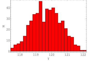
(a)

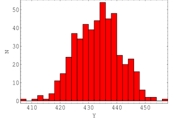
(b)

Figure 6: Histogram probability density for $Y_{1000}$, relative to the hysteresis bifurcation diagram of figure 5 with $U_{o}=73$ and (a): $c=1$, (b): $c=7$. Note that the two densities are located in different ranges of values of $y$.

• if $c<U_{m}-U_{o}$, then the asymptotic value $y_{+\infty}$ will be a random variable with a probability density $\rho(y;c)$ (where we stress the dependence of the density on the parameter $c$) having a maximum corresponding to a low equilibrium point as in figure 6-(a);

• if $U_{o}-c<U_{m}$ and $U_{o}>U_{m}$ we have a $\rho(y;c)$ such that its maximum is near to an upper equilibrium point.

• when $c>U_{m}-U_{o}$, we may find an $\epsilon>0$ such that if $c<(U_{m}-U_{o})(1+\epsilon)$ the above density remains unchanged, whereas if $c>(U_{m}-U_{o})(1+\epsilon)$ the above probability density $\rho(y;c)$ changes, since its maximum is now near to an upper equilibrium point, as in figure 6-(b).

This changing in the probability density distribution of $y_{\infty}$ (as well as the change in the behaviors summarized at the end of section 3.2) has been called noise-induced transition [5] or, in recent literature, stochastic bifurcation [6]. From a computational point of view, in practice we approximate $\rho(y_{\infty};c)$ with the probability density distribution of a $y_{G}$ with $G>>1$. It results that the nearer $c$ is to $U_{m}-U_{o}$, the greater the value of $G$ which has to be chosen. On the contrary if one establishes a priori a finite number of generations $\hat{G}$, there are two values $c_{1}>U_{m}-U_{o}$ and $c_{2}>c_{1}$ such that if $c<c_{1}$ the probability density of $y(\hat{G})$ has a low peak, if $c>c_{2}$ it has an high peak and if $c_{1}<c<c_{2}$ it has two peaks: one low and one high.

3.4 Mixed behaviors

Remaining in the framework of increasing $\beta(y)$, there may be the theoretical possibility to have more complex configurations. In fact, if $\beta(y)$ has $m\geq 2$ inflexion points and if it is $2(t_{o}/t_{1})\beta(+\infty)>1$, there may be $n\leq m$ stable equilibria and $n$ unstable equilibria (in alternated sequence starting from a stable equilibrium: STABLE , UNSTABLE, STABLE, UNSTABLE,etc$\dots$). Proceeding as in the sections 3.1 and 3.3, it is easy to show that there are $n-1$ hysteresis bifurcations followed by a final saddle-node bifurcation. Thus also in this more complex case, it is possible to find a threshold value $U_{m}$ exceeding which there is exponential explosion. When $2(t_{o}/t_{1})\beta(+\infty)<1$, there may be $n+1$ stable equilibria and $n$ unstable equilibria, and $n$ hysteresis bifurcations. Summarizing, also in these more complex case, the biological findings previously illustrated do not change, since the behavior is simply a mix of the behaviors illustrated in the two previous subsections.

4 Non-linear model: contribution to the rate of PCD by both the semi-differentiated and the differentiated cells

The first natural extension to the proposed nonlinear model is to consider that both semi-differentiated and fully differentiated cells may contribute to the variability in PCD. Therefore we have

$$\beta_{1}(y,z),\beta_{2}(y,z),\beta_{3}(y,z)$$

with:

$$\frac{\partial\beta_{1}}{\partial y}<0,\frac{\partial\beta_{1}}{\partial z}<0,\frac{\partial\beta_{2}}{\partial y}\geq 0,\frac{\partial\beta_{2}}{\partial z}\geq 0,\frac{\partial\beta_{3}}{\partial y}>0,\frac{\partial\beta_{3}}{\partial z}>0$$

For example, by assuming that there is no difference in the contribution of the semi-differentiated and fully differentiated cells, a natural candidate function is

$$\beta_{3}^{o}(y+z)$$

where $\beta_{3}^{o}(.)$ is a function shaped as the one in figure 1 (different contribution may be modeled by assigning to $y$ and $z$ two different positive weights: $\beta_{3}^{o}(w_{y}y+w_{z}z)$, e.g. $w_{y}=0$ and $w_{z}=1$ i.e. dependence only on the fully differentiated cells). The following model results

$$x_{G+1} = 2\alpha_{3}x_{G}$$

$$y_{G+1} = 2\frac{t_{o}}{t_{1}}\beta_{3}(y_{G}+z_{G})y_{G}+2\alpha_{2}x_{G}$$ (5)

$$z_{G+1} = 2\frac{t_{o}}{t_{1}}\beta_{2}(y_{G}+z_{G})y_{G}+(1-\gamma\frac{t_{o}}{t_{2}})z_{G}$$

Note that:

$$\frac{\partial y_{G+1}}{\partial z_{G}}>0,\frac{\partial z_{G+1}}{\partial y_{G}}\geq 0$$

that is, mathematically, the system may be classified as cooperative, in agreement with what we suggested biologically . Defining the new variable:

$$s_{G}=y_{G}+z_{G}$$

(note that $s_{G}$ it is such that $s_{G}\geq y_{G}$ and $s_{G}\geq z_{G}$) and summing the third and the second equation of (4) we obtain (for constant $U=\alpha_{2}x_{G}$):

$$y_{G+1} = 2\frac{t_{o}}{t_{1}}\beta_{3}(s_{G})y_{G}+U$$ (6)

$$s_{G+1} = 2\frac{t_{o}}{t_{1}}(\beta_{2}(s_{G})+\beta_{3}(s_{G}))y_{G}+(1-\gamma\frac{t_{o}}{t_{2}})(s_{G}-y_{G})+U$$

whose equilibrium points are determined by the equation

$$2\frac{t_{o}}{t_{1}}\beta_{3}(s)=1-\frac{U}{s}\big{(}1+2*\frac{t_{2}}{\gamma t_{1}}\beta_{3}(s)\big{)}$$ (7)

which is very similar to equation (3) and which leads to the same bifurcation curves. Simulations did not show a qualitative difference between non-cooperation and cooperation. From a quantitative point of view, on the contrary, there are differences: the dynamics are faster in the co-operative model, in agreement with the fact that $\beta_{3}$ depends on the sum $y+z$.

5 Dependence of the parameters on ratio of semi-differentiated to stem cells

If we suppose that the parameters do not depend directly on $y$, but that they depend, for example, on the ratio:

$$\frac{y}{x}$$

we obtain, because of the constance of the $x_{G}$, similar results as far as concerns the bifurcation diagrams. In fact, if we define the new variable:

$$\varrho=\frac{y}{X}$$ (8)

we may write the equilibrium equation in the form:

$$2\frac{t_{o}}{t_{1}}\beta_{3}(\varrho)=1-\frac{2\alpha_{2}}{\varrho}$$ (9)

the only difference in this case being that the bifurcation parameter is no longer $U=2X\alpha_{2}$, but is now the parameter $\alpha_{2}$ alone. As consequence of (8), the equilibrium value is proportional to $X$. again the same bifurcation diagram holds also by proposing a dependence on the following ratio:

$$\frac{y}{y+X}$$

the equilibrium equation may be written as:

$$2\frac{t_{o}}{t_{1}}\beta_{3}(\frac{\varrho}{\varrho+1})=1-\frac{2\alpha_{2}}{\varrho}$$ (10)

which leads to the same bifurcation diagram because of the geometrical properties of the function $\varrho/(\varrho+1)$ and $\beta_{3}$.

6 Conclusions

We have presented a development of our model of cell birth, differentiation and death in the colonic crypt, which was used as a model for tumorigenesis. Our previous model, which was linear, showed that failure of PCD - for example, in tumorigenesis - could lead either to exponential growth in cell numbers or to growth to some plateau. We note here that, remaining in the linear framework, some biological noteworthy modifications are possible. In particular: periodic or random changes of the parameters, in order to take into the account interactions with the microenvironment; and, as suggested by one of the referees, incorporating exponential decay in the growth parameter, as in the Gompertz model [8]. This second point, in particular, would deserve a further analysis, also in the non-linear case.
Our new models have incorporated realistic fluctuation in the parameters of the model and have introduced non-linearity by assuming dependence of parameters on the numbers of cells in each state of differentiation, perhaps as a result of a mutation occurring in and spreading through the stem cell population. Furthermore, recently in [8] it has been proposed for cancer cells a mechanism of self organization through cell to cell communication similar to the quorum sensing of bacteria, and other kind of cell-density dependence of apoptosis has been proposed in [9] and [10]. Our new models are characterized by bifurcation between increase in cell numbers to stable equilibrium or explosive exponential growth, although, in particular cases, two coexisting stable equilibria exist together with an unstable equilibrium (see sect. 3.1). Moreover, we note here that for more complex (but increasing) shapes of $\beta(y)$, there may be even other coexisting equilibria. However, it is easy to show that these more complex (and quite theoretical) configurations of equilibria do not alter the biological findings of the present work.
If we assume fluctuation in cell numbers undergoing PCD (whether determined or random), the incorporation of non-linearity into the model generally makes exponential growth of a tumor more likely, as long as (for random fluctuation), the number (or the proportion) of cells progressing from a stem cell to a semi-differentiated state exceeds a certain critical value for a sufficiently long period of time. In most - but not all - cases, once exponential growth has started, this process is irreversible. In some circumstances, exponential growth may be preceded by a long plateau phase, mimicking equilibrium, of variable duration: thus apparently self-limiting lesions may not be so in practice and the duration of growth of a tumor may be impossible to predict on the basis of its size. Our results show that the consequences of failure of PCD are complex and difficult to predict. Progression of a tumor is not necessarily caused by acquiring additional extra genetic or epigenetic changes, but may simply be a consequence of ’normal’ alterations in cell turnover or fluctuations in numbers, owing to, for example, tissue damage. Apparent regression of tumors may occur similarly. While failure of PCD is more likely than simple increased cell replication to be associated with benign, generally non-progressing tumors, the exponential growth observed suggests that PCD failure is potentially a general mechanism of carcinogenesis.

7 Acknowledgements

We wish to thank an anonymous referee for her/his valuable comments.

Figure 1: Non-linear model of section 4: plots of $2\frac{t_{o}}{t_{1}}\beta_{3}(y)$. Upper: $2\frac{t_{o}}{t_{1}}\beta_{3}(+\infty)>1$, lower $2\frac{t_{o}}{t_{1}}\beta_{3}(+\infty)<1$

Figure 2: Excess of self-renewal of semi-differentiated cells ($2\frac{t_{o}}{t_{1}}\beta_{3}(+\infty)>1$). There are 2 (for $U<U_{m}$) or or 0 ($U>U_{m}$) equilibria. In the limit case $U=U_{m}$ there is tangency (a double equilibrium point). The higher the values of $U$, the further to the right are the hyperbolae.

(a)

(b)

Figure 3: (a): Typical saddle node diagram corresponding to figure 2: for $U<U_{m}$ there are 2 equilibria (one stable, the lower, and one unstable) and for $U>U_{m}$ no equilibria exist, (b): simulation corresponding to a value of $U$ slightly less than the critical value $U_{m}$; (c): simulation corresponding to a value of $U$ slightly greater than the critical value $U_{m}$, which implies exponential explosion.

Figure 4: No excess of self-renewal of semi-differentiated cells ($2\frac{t_{o}}{t_{1}}\beta_{3}(+\infty)<1$). There are 1 (for $U<U_{m}$ and for $U>U_{M}$) or 3 ($U_{m}<U<U_{M}$) equilibria. In the limit cases $U=U_{m}$ and $U=U_{M}$ there is tangency (a double equilibrium point). The higher the values of $U$, the further to the right are the hyperbolae.

(a)

(b)

(c)

Figure 5: (a): Typical Hysteretic Global Bifurcation diagram: 2 local saddle node in a S-shaped curve (associated with fig. 4). Simulations corresponding to (a): a value of $U$ slightly less than the critical value $U_{M}$; (b) a value of $U$ slightly greater than the critical value $U_{M}$.

References

- [1] Tomlinson I.P.M. Bodmer W.F. Failure of Programmed Cell Death and differentiation as causes of tumors: Some simple mathematical models. Proc. Natl. Acad. Sci. USA 92, - .
- [2] Bodmer W.F. Tomlinson I.P.M. Population Genetics of Tumours in Variations in human genome - Cyba foundation Symposium 1997 ( eds: Agarwal, S. and Zhang, R ), 181-193. Chicester UK: Wiley.
- [3] Lasota A. McCay M.C. Statistical aspects of dynamics. Heidelberg: Springer-Verlag.
- [4] Hale J.K. Kocac H. Dynamics and bifurcations. Heidelberg: Springer-Verlag.
- [5] Horsthemke W. Lefever R. Noise-Induced Transitions. Theory and Applications in Physics, Chemistry, and Biology. Heidelberg: Springer-Verlag.
- [6] Arnold L. Random Dynamical Systems. Heidelberg: Springer-Verlag.
- [7] Wiggins S. Introduction to Applied non-linear Dynamical Systems and Chaos. Heidelberg: Springer-Verlag.
- [8] M. Molski J. Konarski, Coherent states of Gompertzian growth, Physical Review E,68 Art. No. 021916 Part 1 AUG (2003)
- [9] A. Yates R. Callard death and the maintenance of immunological memory. DCDS - B 1, - .
- [10] K. Hardy H. Stark Mathematical models of the balance between apoptosis and proliferation. Apoptosis 7, - .