A general framework for modeling tumor-immune system competition and immunotherapy: mathematical analysis and biomedical inferences.

Abstract

In this work we propose and investigate a family of models, which admits as particular cases some well known mathematical models of tumor-immune system interaction, with the additional assumption that the influx of immune system cells may be a function of the number of cancer cells. Constant, periodic and impulsive therapies (as well as the non-perturbed system) are investigated both analytically for the general family and, by using the model by Kuznetsov et al. (V. A. Kuznetsov, I. A. Makalkin, M. A. Taylor and A. S. Perelson. Nonlinear dynamics of immunogenic tumors: Parameter estimation and global bifurcation analysis. Bulletin of Mathematical Biology,56(2) 295-321, (1994)), via numerical simulations. Simulations seem to show that the shape of the function modeling the therapy is a crucial factor only for very high values of the therapy period $T$, whereas for realistic values of $T$, the eradication of the cancer cells depends on the mean values of the therapy term. Finally, some medical inferences are proposed.

¹ Department of Epidemiology and Biostatistics, European Institute of Oncology, Via Ripamonti 435, Milano, Italy, I-20141
EMAIL: alberto.donofrio@ieo.eu, PHONE:+390257489819
Keywords: Cancer – Immunotherapy – Stability Theory – Periodical forcing

1 Introduction

Millions of people die from cancer every year [1]. And worldwide trends indicate that millions more will die from this disease in the future [2]. Great progress has been achieved in fields of cancer prevention and surgery and many novel drugs are available for medical therapies [3, 4, 5]. Biophysical models may prove to be useful in oncology not only in explaining basic phenomena [6, 7], but also in helping clinicians to better and more scientifically plan the schedules of the therapies [7, 8]. An interesting therapeutic approach is immunotherapy [4, 5], consisting in stimulating the immune system in order to better fight, and hopefully eradicate, a cancer. In particular, in this paper I will be referring to generic immunostimulations, for example via cytokines, but for the sake of simplicity I will use the term ”immunotherapy”. The basic idea of immunotherapy is simple and promising, but the results obtained in medical investigations are globally controversial [9, 10, 11, 12], even if in recent years there has been evident progress. From a theoretical point of view, a large body of research has been devoted to mathematical models of cancer-immune system interactions and to possible applications to cure the disease [13, 14, 16, 17, 18, 19, 20, 21, 22, 23, 24] (and references therein). Analyzing the best known finite dimensional models [13, 14, 16, 20, 23], we note that their main features are the following:

• Existence of a tumor free equilibrium;

• Depending on the values of parameters, there is the possibility that the tumor size may tend to $+\infty$ or to a macroscopic value;

• Possible existence of a ”small tumor size” equilibrium, which coexists with the tumor free equilibrium.

An ”accessory” feature is the existence of limit cycles [16]. From this rough summary, one may understand that the puzzling results obtained up to now by immunotherapy [9] may be strictly linked to the complex dynamical properties of the immune system-tumor competition. In general, it happens that the cancer-free equilibrium coexists with other stable equilibria or with unbounded growth, so that the success of the cure depends on the initial conditions, and - even theoretically - it is not always granted.

2 A general family of models and its properties

In [22], Sotolongo-Costa et al. proposed the following very interesting Volterra-like model (similar to the one in [20]) for the interaction between a population of tumor cells (whose number is denoted by $X$) and a population of lymphocyte cells ($Y$) :

$$X^{\prime} = aX-bXY$$ (1)

$$Y^{\prime} = dXY-fY-kX+u+P(t),$$ (2)

where the tumor cells are supposed to be in exponential growth (which is, however, a good approximation only for the initial phases of the growth) and the presence of tumor cells implies a decrease of the ”input rate” of lymphocytes. System (1)-(2) may be rewritten in non-dimensional form [22]:

$$x^{\prime} = \alpha x-xy$$ (3)

$$y^{\prime} = xy-\frac{1}{\alpha}y-kx+\sigma+p(t)$$ (4)

(in short notation $(x^{\prime},y^{\prime})=C(x,y)$). The function $p(t)\geq 0$ is assumed periodic with period $T$ and it models the effect of immunotherapy. The model has been studied in depth both in the case of absence of therapy and in the case of therapy by using the test function $p(t)=0.5F(1+cos(4\pi\nu t))$.

The model shows two equilibria (one of which is tumor-free) and also unbounded growth. However, the system (3)-(4) allows negative solutions for non small $x$, which is not physically acceptable. In fact:

$$C(x,0)=(ax,\sigma+p(t)-kx)$$ (5)

implies that for $x>(\sigma+p_{max})/k$ it is $C(x,0).(0,-1)>0$, and $y(t)$ becomes negative in finite times. Furthermore, the second equilibrium point is a consequence of the negativity of $\sigma-kx$.

The model in [22], though it has this problem of lack of physical consistency, is, however, of great interest because the killing of lymphocytes is seen as function of the $x$ variable Alternatively, the influx of lymphocytes may be thought of as a function of the entity of the disease, which we will denote as $Q(x)$. Indeed, it has been observed that in some cases cancer progression may cause generalized immunosuppression. See [25] and references therein. See [25] and references therein. Thus, in [22] it is $Q(x)=\sigma(1-(k/\sigma)x)$, which may be read as a first order Taylor approximation of a more general non-increasing function.

However a general influx function is only one of the possible modifications of model (3)-(4): there may be others, which are also biologically reasonable. One might take into the account many factors: different functional forms for the interaction term, saturation in the predation term and, mainly, non exponential growth of the cancer: logistic, gompertzian, generalized logistic etc $\dots$ All these modifications are reasonable and useful. Thus, I think that it might be useful to define and study the following general family of models:

$$x^{\prime} = x(\alpha f(x)-\phi(x)y)$$ (6)

$$y^{\prime} = \beta(x)y-\mu(x)y+\sigma q(x)+\theta(t)$$ (7)

where:

• $x$ and $y$ are the non-dimensionalized numbers of, respectively, tumor cells and of effectors cells of immune system;

• $0<f(0)\leq+\infty$, $f^{\prime}(x)\leq 0$ and in some relevant cases we shall suppose that it exists an $0<\overline{x}\leq+\infty$ such that $f(\overline{x})=0$), $Lim_{x\rightarrow 0^{+}}{xf(x)}=0$. Thus, $f(x)$ summarizes many widely used models of tumor growth rates, such as the Exponential model: $f(x)=1$ [7], the Gompertz: : $f(x)=Log(A/x)$ [7, 50] and its generalizations [7, 50], the Logistic model: $f(x)=1-x/A$ [50], the Hart-Schochat-Agur: $f(x)=x^{-\gamma}\textrm{, }0<\gamma<1$ [26], the von Bertanlaffy: $f(x)=x^{-1/3}-b$ [50, 53], the Guiot’s et al. model: $f(x)=x^{3/4}-b$ [27], the linear growth model by Bru and coworkers[28] which may be written as follows: $f(x)=x^{-1/3}$ (note that it may be considered a particular case of the von Bertalaffy model and of the Hart-Shochat-Agur model) etc$\dots$

• $\phi(x)>0$, $\phi(0)=1$, $\phi^{\prime}(x)\leq 0$ and $x\phi(x)\rightarrow l\leq+\infty$;

• $q(x)$ is such that $q(0)=1$ (as a consequence $\sigma=Q(0)$) and it may be non-increasing or also initially increasing and then decreasing, i.e. we may assume that either the growth of tumor decreases the influx of immune cells or that, on the contrary, it initially stimulates the influx);

• $\beta(x)\geq 0$, $\beta(0)=0$ and $\beta^{\prime}(x)\geq 0$;

• $\mu(x)>0$ and $\mu^{\prime}(x)>0$.

For the sake of simplicity we define the following function $\Psi(x)=\mu(x)-\beta(x)$ and write:

$$x^{\prime} = x(\alpha f(x)-\phi(x)y)$$ (8)

$$y^{\prime} = -\Psi(x)y+\sigma q(x)+\theta(t).$$ (9)

$\Psi(x)$ is assumed to be positive, otherwise it may be positive in $[0,x_{1})\cup(x_{2},+\infty)$ with $\Psi(x_{1})=\Psi(x_{2})=0$. We may assume that it has an absolute minimum in $[0,+\infty)$. We may use $\Psi(x)$ to classify the tumors depending on their degree of aggressiveness against the immune system:

• $\Psi(x)>0$: in such a case the ability of destroying immune cells is never won by the stimulatory effect on the immune system, therefore the tumor may be indicated as ”highly aggressive”/”lowly immunogenic”;

• Variable sign $\Psi(x)$: since in such a case the destruction of cells may be compensated by the stimulatory effect, we will refer to such a tumors as ”lowly aggressive”/”highly immunogenic”.

The above model includes as particular cases the models [13, 14, 20, 23]. For instance, the Stepanova model [13] is such that $f(x)=1$, $\phi(x)=1$, $\beta(x)=\beta_{1}x$, $q(x)=1$ and $\mu(x)=\mu_{o}+\mu_{2}x^{2}$; the de Vladar-Gonzalez model [23] is similar, but: $f(x)=Log(K/x)$.

Note that Nani and Freedman proposed an interesting model of adoptive cellular immunotherapy in which generic functions are used [19]. However, their approach differs from ours since in their model the proliferation of cells of the immune systems is not stimulated by cancer cells. In other words in the Nani and Freedman model the interaction tumor cells - immune system is only destructive for immune cells. Furthermore, in their model the ”loss rates” are proportional (in our notation we might write $\mu(x)=\mu(0)+const\phi(x)$).

In the absence of treatment, system (8)-(9) admits the existence of a cancer free equilibrium $CF=(0,\sigma/\Psi(0))$.

If $f(0)<+\infty$, we have that if $\sigma>\sigma_{cr}=\alpha\Psi(0)f(0)/\phi(0)$ $CF$ is locally asymptotically stable (LAS), unstable if $\sigma<\sigma_{cr}$. Biologically, $\sigma>\sigma_{cr}$ means that the immune system works very well and that it is able to destroy small tumors. On the contrary $\sigma\approx 0$ means that there is immunodepression.

Furthermore, when $\phi(x)=constant=\varphi$ and $\Psi(x)\leq\Psi^{*}<+\infty$, if $\sigma>\sigma^{*}=\alpha f(0)\Psi^{*}/(q_{min}\varphi)$ it follows that $CF$ is globally asymptotically stable ($GAS$). In fact, from $y^{\prime}=-\Psi(x)y+\sigma q(x)\geq-\Psi^{*}y+\sigma q_{min}$ if follows that asymptotically $y(t)\geq\sigma q_{min}/\Psi^{*}$. As a consequence, asymptotically $x^{\prime}\leq(\alpha f(0)-\varphi(\sigma q_{min}/\Psi^{*}))x$, i.e. if $\sigma>\sigma^{*}$ it is $x(t)\rightarrow 0\Rightarrow y(t)\rightarrow\sigma/\Psi(0)$.

A relevant problem, up to now, is that the immunotherapeutic agents are characterized by strong toxicity, thus $\sigma>\sigma^{*}$ might be too biologically high, even in cases in which when it is mathematically small.

If $f(0)=+\infty$, as in the Gompertzian case (used, for example, in [23]) and in other tumor growth models, then $CF$ is unstable anyway (as previously stressed for the particular model [23]) because in such a cases the derivative of $xf(x)$ at $x=0$ is $+\infty$. In the light of [23] and of our generalization, this implies that the immune system would never be able to totally suppress even the smallest tumor cell aggregates, which is a very strong inference. This instability result deserves some comments because it has deep medical implications: the impossibility to completely recover from any type of tumors whatsoever. On the contrary, it is commonly held that the immune system may be able, in some cases, to kill a relatively small aggregate of cancer cells. In the background of all cancer therapies (which are of finite duration) there is the implicit hypothesis that the drug will kill the vast majority of the malignant cells and that the relatively few residual cells may in some cases be killed by the immune system [32]. Accepting this hypothesis, the equilibrium $CF$ should have the possibility to be LAS and, as a consequence, for small $x$ the function $f(x)$ should be bounded.

The modeling of cancer by means of the Gompertz law of growth was introduced in early sixties by A. K. Laird [33, 34]. She conducted pioneering data-fitting work using a vast amount of real data and justified the law in terms of increasing mean generation time. There is much research showing that the Gompertzian model fits data well from experimental and in vivo tumors [36, 35, 37, 38, 39, 40, 41]. From a theoretical point of view, Gyllenberg and Webb [42], Calderon and Kwembe [43], Calderon and Afenya [44, 45] proposed physico-mathematical justification of the Gompertz model. Furthermore, some interesting physical properties of the Gompertz model have been elucidated by Konarski and Molski [46] and by Konarski and Waliszewski [47].

However, the doubling time of a population of cells cannot be lower than the minimal time needed by a cell to divide, which is obviously non-null. This biological constraint is in contrast with the unboundedness of $f(x)$ in the Gompertz and other models, as stressed by Wheldon [7]. More recently, inconsistency at low number of cells have been recognized by Castorina and Zappala’ in their derivation of the Gompertizan model based on methods of statistical mechanics [48, 49]. They showed that the validity of the Gompertz model starts above a minimum threshold for the number of cells, whereas under the threshold there is exponential growth. In other words, they derived biophysically the Gomp-Ex model proposed on biological ground in [54, 7]. Using data from multicellular tumor spheroids, Marusic and coworkers performed a systematic comparison of many models [50], which showed that Gompertz’s model fitted their data very well, but slightly less well than the Piantadosi model [55], which has finite $f(0)$. Furthermore, in their fittings, it was not possible to discriminate between the pure Gompertz model and the Gomp-Ex model. Demicheli and coworkers used Gomp-Ex model on in vitro and in vivo data obtaining results strongly supporting this model [52]. Other comparisons may be found in [44, 53]. Moreover, in general, van Leeuwen and Zonneveld [51] claims that it may be not possible to discriminate between exponential, logistic and gompertzian models in the early phases of growth. Recent experimental studies conducted by Bru and coworkers support an initial phase of exponential growth [28]. Summarizing, I consider the results by de Vladar and Gonzalez (and our extensions) to be very valuable, but they may be read in a dichotomic way:

• A tumor is permanent: the innate immune surveillance is never able to completely eradicate even the smallest tumor.

• Since there is relevant evidence that the immune system is able in some cases to eliminate small tumors [57, 58] (as we will see in following sections, the ability of eradicate the disease or not depends on initial conditions), the properties of the de Vladar-Gonzalez model (and of our extension) may be seen as an evidence that Gompertzian and other models characterized by $f(0)=+\infty$ are not appropriate for very small tumors, in coherence with [7, 48, 49, 28].

In case of the absence of influx of immune cells ($q(x)=0$) and for laws of growth in which $\overline{x}$ exists, there is a different particular equilibrium point, which we shall call ”immune free”: $IF=(\overline{x},0)$, which is LAS.

Other multiple non null equilibria may be found by finding the positive intersection of the two nullclines:

$$y_{C}(x) = \alpha\frac{f(x)}{\phi(x)}$$ (10)

$$y_{I}(x) = \frac{\sigma q(x)}{\Psi(x)}.$$ (11)

The functions $y_{C}(x)$ and $y_{I}(x)$ are useful in the determination of the LAS of the equilibria , since the characteristic polynomial of the Jacobian, calculated at a given equilibrium point $(x_{e},y_{e})$, is:

$$\lambda^{2}+\Big{(}\Psi(x_{e})-x_{e}\phi(x_{e})y_{C}^{\prime}(x_{e})\Big{)}\lambda+\Psi(x_{e})x_{e}\phi(x_{e})\Big{(}-y_{C}^{\prime}(x_{e})+y_{I}^{\prime}(x_{e})\Big{)}=0.$$ (12)

So the LAS condition is:

$$y_{C}^{\prime}(x_{e})<\frac{\Psi(x_{e})}{x_{e}\phi(x_{e})}\textrm{ AND }y_{I}^{\prime}(x_{e})>y_{C}^{\prime}(x_{e}).$$ (13)

Note that the first part of the AND condition is automatically fulfilled when $y^{\prime}_{C}(x)\leq 0$ (because $x_{e}$ cannot lie in an interval where $\Psi(x)<0$), whereas the second part has a straightforward geometrical interpretation.

Finally, it is interesting to note that the above family of model may admit limit cycles if $f(x)=1$ (exponential growth) and $q(x)$ is identically null for $x>x_{q}$ with $x_{q}<x_{1}$. In fact, in such a case there is the equilibrium point $(x_{1},\alpha)$ whose characteristic polynomial is:

$$\lambda^{2}+h^{2}=0\textrm{, }h^{2}:=-x_{1}\Psi^{\prime}(x_{1})\alpha>0$$ (14)

In effect, some cases of sustained oscillations (or slow oscillations with very small damping) have been reported in the medical literature [29, 30, 31]. Periodic solutions in absence of influx of immunocompetent cells are predicted also in [16].

On the contrary, if $y^{\prime}_{C}(x)\leq 0$ (for example when $\phi(x)$ is constant), by applying the Dulac-Bendixon theorem with multiplicative factor $1/(xy\phi(x))$ (as in the specific models [14, 20]) one obtains that the presence of limit cycles is not possible. In fact:

$$Div\Big{(}\frac{1}{xy\phi(x)}(x^{\prime}(x,y),y^{\prime}(x,y))\Big{)}=\frac{\alpha y_{C}^{\prime}(x)}{y}-\sigma\frac{q(x)}{x\phi(x)y^{2}}<0$$ (15)

2.1 The global behavior

In some important cases, it is possible to study the global behavior of the family, by means of differential inequalities and of the Poincare-Bendixon trichotomy [56]. We may state the following simple propositions:

1. When $\Psi(x)>0$ and $f(x)=1$ and $y_{C}^{\prime}(x)\geq 0$, if it is $y_{I}(x)<y_{C}(x)$ then $x(t)\rightarrow+\infty$. Proof: Let us define $y_{I}^{MAX}:=Max_{x\in\mathbb{R}_{+}}y_{I}(x)$ and $x_{M}$ such that $y_{I}(x_{M})=y_{I}^{MAX}$. If it is $y_{I}(x)<y_{C}(x)$ it is easy to show that the set $H=\Big{\{}(x,y)|x>x_{M}\textrm{ AND }0\leq y\leq y_{I}^{MAX}\Big{\}}$ is positively invariant and adsorbing. Thus, since in $H$: $x^{\prime}\geq x\phi(x)(y_{C}(x_{M})-y_{I}^{MAX})>0$, it follows readily that $x(t)\rightarrow+\infty$;

2. It $\Psi(x)>0$, it exists $\bar{x}$ such that $f(\bar{x})=0$ , $y_{C}^{\prime}(x)<0$ and there is a unique LAS equilibrium point $S=(x_{e},y_{e})$ , then $S$ is GAS. Proof: Let us define $y_{I}^{MAX}:=Max_{x\in[0,\overline{x}]}y_{I}(x)$ and $y_{I}^{min}:=Min_{x\in[0,\overline{x}]}y_{I}(x)$. Furthermore, if $f(0)>y_{I}^{MAX}$ let it be $\tilde{x}=y_{I}^{-1}(y_{I}^{MAX})$, if $f(0)\leq y_{I}^{MAX}$ let it be $\tilde{x}=0$. Since $\Psi(x)(y_{I}^{min}-y)\leq y^{\prime}\leq\Psi(x)(y_{I}^{MAX}-y)$ it is easy to see that the set $R=\Big{\{}(x,y)|\tilde{x}<x\leq\overline{x}\textrm{ AND }y_{I}^{min}\leq y\leq y_{I}^{MAX}\Big{\}}$ is positively invariant and adsorbing and contains $S$. Since we have ruled out the possibility that there may be limit cycles, as a consequence $S$ is $GAS$.

3. When $\Psi(x)>0$ and $y_{C}^{\prime}(x)$ is non-constant and there is a unique LAS equilibrium point $S=(x_{e},y_{e})$, if it holds also that

   $$y_{C}^{Max}>y_{I}^{Max}$$ (16)

   then $S$ is $GAS$. Proof: When $f(x)$ is unbounded, one may see that, there may be a relative minimum followed by a relative maximum in $(0,\overline{x})$. On the contrary, when $f(x)$ is bounded, there is an absolute maximum. Calling now $x^{*}$ the point in which $y_{C}(x)$ is (absolutely or relatively) maximum, one has that $R^{*}=\Big{\{}(x,y)|x^{*}\leq x\leq\overline{x}\textrm{ AND }y_{I}^{min}\leq y\leq y_{I}^{MAX}\Big{\}}$ is positively invariant and adsorbing, contains $S$. Since in $R^{*}$ it is $y_{C}^{{}^{\prime}}(x)\leq 0$ ( which implies that closed orbits are ruled out), as a consequence, $S$ must be GAS.

4. When $\Psi(x)>0$ and $y_{I}(x)>y_{C}(x)$ for $x\in[0,\bar{x}]$ then $CF$ is GAS. Proof: It is a particular case of proposition 2.

5. If $\Psi(x)>0$, there does not exist a $\bar{x}$ such that $f(\bar{x})=0$ , $y_{C}^{\prime}(x)<0$ and there is a unique LAS equilibrium point $S=(x_{e},y_{e})$ , then $S$ is GAS. Proof: Let us define $y_{I}^{MAX}:=Max_{x\in[0,+\infty)}y_{I}(x)$. Let us consider a point $P_{o}=(x_{o},0)$ with $x_{o}>x_{e}$, and the orbit starting from it, which intersects the curve $y_{C}(x)$ in the point $P_{a}=(x_{a},y_{C}(x_{a}))$. Let us consider the following points $P_{b}=(x_{a},y_{I}^{MAX})$, $P_{c}=(0,y_{I}^{MAX})$ and $P_{d}=(0,0)$. The arc of orbit $\widehat{P_{o}P_{a}}$ and the straight segments $\overline{P_{a}P_{b}}$,$\overline{P_{b}P_{c}}$,$\overline{P_{c}P_{d}}$ and $\overline{P_{d}P_{o}}$ bounds an invariant set for our system. As a consequence of the Bendixon-Poincare’ tricothomy we have that S is GAS.

6. When $\Psi(x)$ has variable sign, and $f(x)$ is bounded and $y_{I}(x)>y_{C}(x)$ then $CF$ is $GAS$. Proof: the set $X=\Big{\{}(x,y)|0<x\leq\overline{x}\textrm{ AND }y\geq 0\Big{\}}$ is positively invariant and adsorbing and in it closed orbits are impossible, as we have seen. However it is not a bounded set, so we have to show that all the orbits starting in $X$ are bounded. Firstly, we notice that it cannot be $y(t)\rightarrow+\infty$, since in such a case, being $x^{\prime}=x(\alpha f(x)-y(t))$, it would be $x(t)\rightarrow 0\Rightarrow y(t)\rightarrow\sigma/\Psi(0)$. Furthermore hypothetical solutions such that $minlim_{t\rightarrow+\infty}\textrm{ }y(t)=0$ and $Maxlim_{t\rightarrow+\infty}\textrm{ }y(t)=+\infty$ are not possible since the set $A=\Big{\{}(x,y)|0<x\leq x_{1}\textrm{ AND }y\geq y_{c}(x)\Big{\}}$ is positively invariant. As a consequence of these properties, thanks to the Bendixon-Poincare’ trichotomy, $CF$ is GAS.

7. When $\Psi(x)$ has variable sign, there is $\bar{x}$ such that $f(\bar{x})=0$, $y_{C}(x)<0$ and there is a unique LAS equilibrium point $S$ then $S$ is $GAS$. Proof: the set $X=\Big{\{}(x,y)|0<x\leq\overline{x}\textrm{ AND }y\geq 0\Big{\}}$ is positively invariant and adsorbing and in it closed orbits are impossible, as we have seen. However it is not a bounded set. Let us consider $y_{I}(x)$: it is such that it is split in two branches: $y_{I}^{right}(x)$ for $x_{2}\leq x\leq+\infty$ (which has no intersections with $y_{C}(x)$) and $y_{I}^{left}(x)$ for $0\leq x<x_{1}$ (on which $S$ lies). Let us consider a point $P_{i}=(x_{i},y_{i})$ lying on the curve $(x,y_{I}^{right}(x))$ and having $y_{i}>y_{C}(0)>y_{C}(x_{2})$. Let the orbit starting from $P_{i}$ intersect the graph $(x,y_{I}^{left}(x))$ in a point $P_{f}=(x_{f},y_{f})=(x_{f},y_{I}^{left}(x_{f}))$ (note that it is $y_{f}>y_{i}$). Let us define the following points: $P_{A}=(0,y_{f})$, $P_{B}=(0,\bar{x})$ and $P_{C}=(\bar{x},y_{i})$. It is easy to see that segment of orbit $\widehat{P_{i}P_{f}}$ and the straight segments $\overline{P_{f}P_{A}}$,$\overline{P_{A}O}$, $\overline{OP_{B}}$, $\overline{P_{B}P_{C}}$ and $\overline{P_{C}P_{i}}$ bound an invariant set $\Omega$ for our dynamical system. As a consequence, thanks to the Bendixon-Poincare trichotomy, $S$ is GAS.

8. When the sign of $\Psi(x)$ is variable, there is no $\bar{x}$ such that $f(\bar{x})=0$, $y_{C}(x)<0$ and there is a unique LAS equilibrium point $S$ then $S$ is $GAS$. Proof: The proof is easily obtained by applying methods of propositions 7 and 5 to find a bounded positively invariant set surrounding S.

9. When $\Psi(x)>0$ and $q(x)=0$ then $\forall(x(0),y(0))$ it is $y(t)\rightarrow 0^{+}$. Furthermore, in accordance with the growth law $f(x)$, either the tumor tends to an equilibrium value or it grows unbounded. Proof: Let us define $\Psi_{min}=min_{x\in\mathbb{R}_{+}}\Psi(x)$. If $q(x)=0$ it is $y^{\prime}=-\Psi(x)y\leq\Psi_{min}$ $\Rightarrow y(t)\rightarrow 0^{+}$. Thus, the equation for $x(t)$ becomes asymptotically autonomous, so that, depending on $f(x)$, either $x(t)\rightarrow+\infty$ or $x(t)\rightarrow\bar{x}$ (i.e. in this case the equilibrium $IF=(\bar{x},0)$ is GAS).

10. When $\Psi(x)>0$ and $f(x)=1$ and $\phi(x)=const=\varphi$, and there are two equilibria $S=(x_{e},y_{e})$ (LAS) and $U=(x_{u},y_{u})$ (unstable) and there is a separatrix curve $y=\Sigma(x)$ which does not join S to U, then there are two sets $A$ and $B$ such that if $(x(0),y(0))\in A$ then $(x(t),y(t))\rightarrow S$, whereas if $(x(0),y(0))\in B$ then $x(t)\rightarrow+\infty$. Proof: Let us define $y_{I}^{MAX}:=Max_{x\in\mathbb{R}_{+}}y_{I}(x)$ and $x_{\Sigma}=\Sigma^{-1}(y_{I}^{MAX})$ . As a consequence, the set $A=\Big{\{}(x,y)|0<x<x_{\Sigma}\textrm{ AND }Min(0,\Sigma(x))\leq y\leq y_{I}^{MAX}\Big{\}}$ is positively invariant and in it there are no closed orbits, so if $(x(0),y(0))\in A$ then $(x(t),y(t))\rightarrow S$. It is easy to show that given a $y_{I}(x_{\Sigma})/\varphi<\varrho<\alpha/\varphi$ also the set $B=\Big{\{}(x,y)|x>x_{\Sigma}\textrm{ AND }0\leq y\leq\varrho\Big{\}}$ is positively invariant. Thus, since in $B$: $x^{\prime}\geq x(\alpha-\varrho)$, it easily follows that $x(t)\rightarrow+\infty$;

11. Let it be $\Psi(x)>0$, $y_{c}^{\prime}(x)\leq 0$ and it exists $\bar{x}$ such that $y_{C}(\bar{x})=0$ Let there be 4 equilibria CF (unstable), $S_{l}=(x_{e},y_{e})$ (LAS), $U=(x_{u},y_{u})$ (unstable) and $S_{r}=(x_{e},y_{e})$ (LAS), and let there be a separatrix curve $y=\Sigma(x)$ which does not join $S_{l}$ or $S_{r}$ to U, then there are two sets $A$ and $B$ such that if $(x(0),y(0))\in A$ then $(x(t),y(t))\rightarrow S_{l}$, whereas if $(x(0),y(0))\in B$ then $(x(t),y(t))\rightarrow S_{r}$. Proof: As in the previous proposition $A=\Big{\{}(x,y)|0<x<x_{\Sigma}\textrm{ AND }Min(0,\Sigma(x))\leq y\leq y_{I}^{MAX}\Big{\}}$ is positively invariant and in it there are no closed orbits, so if $(x(0),y(0))\in A$ then $(x(t),y(t))\rightarrow S_{l}$. In this case $B=\Big{\{}(x,y)|0<x<\bar{x}\textrm{ AND }0\leq y\leq Min(\Sigma(x),y_{I}^{MAX})\Big{\}}$, and it is positively invariant as well, and with no closed orbits in it. As a consequence: if $(x(0),y(0))\in B$ then $(x(t),y(t))\rightarrow S_{r}$ ;

Remark A consequence of the fourth proposition is that if $y_{I}^{\prime}(0)>0$ (or $y_{I}^{\prime}(0)=0$ AND $y_{I}^{\prime\prime}(0)>0$) then $\sigma>\sigma_{cr}$ is a sufficient condition for the GAS of the $CF$ equilibrium.

In case of multiple equilibria with $\phi(x)=const$ it may be useful to transform (8)-(9) to a nonlinear oscillator. In fact by setting $z=Log(x)$ it is easy to see that the original family becomes:

$$z^{\prime\prime}+(\bar{\psi}(z)-\bar{f}^{\prime}(z))z^{\prime}+\varphi\sigma\bar{q}(z)-\bar{\psi}(z)\bar{f}(z)=0$$ (17)

where $\bar{\psi}(z)=\psi(E^{z})$ etc$\dots$ By defining the damping coefficient:

$$2\nu(z)=(\bar{\psi}(z)-\bar{f}^{\prime}(z))$$ (18)

and the pseudo-potential:

$$U(z)=\int_{0}^{z}{\Big{(}\varphi\sigma\bar{q}(s)-\bar{\psi}(s)\bar{f}(s)\Big{)}ds}$$ (19)

and the total pseudo-energy:

$$E_{tot}=\frac{(z^{\prime})^{2}}{2}+U(z)$$ (20)

it follows immediately that when $\nu(z)>0$:

• Let it be $\bar{x}<+\infty$ and let there be three equilibria $z_{l}<z_{c}<z_{r}$ which are, respectively LAS, unstable and again LAS. Let it be $E_{tot}(0)<U(z_{c})$, then $z(0)<z_{c}$ $\Rightarrow$ $z(t)\rightarrow z_{l}$, whereas $z(0)>z_{c}$ $\Rightarrow$ $z(t)\rightarrow z_{r}$;

• Let it be $\bar{x}=+\infty$ and let there be two equilibria $z_{l}<z_{c}$ which are, respectively LAS and unstable. Let it be $E_{tot}(0)<U(z_{c})$, then $z(0)<z_{c}$ $\Rightarrow$ $z(t)\rightarrow Z_{l}$, whereas $z(0)>z_{c}$ $\Rightarrow$ $z(t)\rightarrow+\infty$.

3 On immunotherapies

3.1 Therapy schedulings

A realistic anticancer therapy may be modeled with sufficient approximation as constant (e.g. via a constant intravenous infusion) or periodic (e.g. the agent is delivered each day as a bolus):

$$\theta(t)=\theta_{m}+\Omega(t)\geq 0\textrm{, }\theta(t+T)=\theta(t),\theta_{m}=\frac{1}{T}\int_{0}^{T}{\theta(t)dt}$$ (21)

For humans, typical periods ranges between $8$ hours to $7$ days [9, 5]. A particular case of periodic therapy is pulsed therapy, i.e. a therapy which induces an instantaneous increase of the number of lymphocytes:

$$\theta(t)=\gamma\sum_{n=0}^{+\infty}{\delta(t-nT)}$$ (22)

In the case of constant infusion therapy (CIT) ($\theta(t)=\theta_{m}$) by defining:

$$\widehat{\sigma}:=\sigma+\theta_{m},\widehat{q}(x):=\frac{\sigma+\theta_{m}}{\widehat{\sigma}}$$ (23)

Remark In the next subsections some asymptotic analyses of therapies shall be conducted. The meaning of the underlying $t\rightarrow+\infty$ limits is the following: the therapies are administered for a time interval $[0,t_{f}]$ which is finite but sufficiently high to guarantee that the number of cancer cells is zero or that other targets have been reached.

3.2 Continuous infusion therapy

All the considerations we have done the absence of therapy hold also in case of CIT. In particular, for $f(0)<+\infty$, the condition for the LAS of the cancer-free equilibrium is:

$$\sigma+\theta_{m}>\sigma_{cr}$$ (24)

Because of the co-presence of other equilibria, the above criterion is not global, i.e. the immunotherapy is not able to guarantee the disease eradication from whatever initial values $(x(0),y(0))$. However, observing that in models in which $\Psi(x)>0$:

$$y_{I}^{withtherapy}(x)=\frac{\sigma q(x)+\theta_{m}}{\Psi(x)}>y_{I}^{notherapy}(x)$$ (25)

(e.g. in Stepanova’s model with low $\mu_{1}$) it happens that, roughly speaking, the stable equilibrium size of the cancer becomes smaller and the unstable equilibria greater, so that the basin of attraction of the unbounded solution is reduced.

Let us consider now some typical situations in case of $y_{C}^{\prime}(x)<0$:

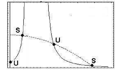
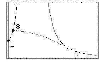
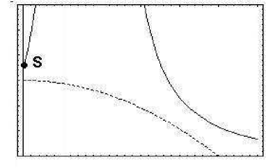
Figure 1: Illustration of the effect of a CIT on a typical configuration in a lowly aggressive tumor. The case is shown in which $\theta_{r}<\theta_{cf}$. $y_{I}(x)$ is plotted as a solid line, whereas $y_{c}(x)$ is dashed. The equilibria are plotted as black points and they are labeled $U$ when unstable, otherwise $S$. First subfigure: figure: in the absence of therapy there are four equilibria among which CF. Second subfigure: with a therapy with $\theta_{r}<\theta<\theta_{cf}$ CF is unstable and coexists with a microscopic tumor equilibrium which is GAS. Fourth subfigure: for a high dose therapy $\theta>\theta_{cf}$ CF becomes GAS.

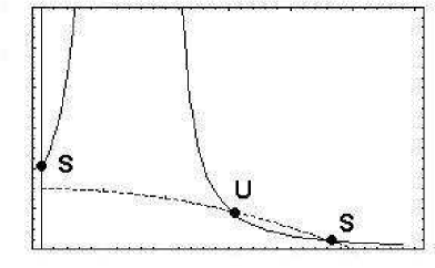
Figure 2: Illustration of the effect of a CIT in a low aggressive tumor for $\theta_{cf}<\theta_{r}$ and $\theta_{cf}<\theta<\theta_{r}$. Symbols as in figure 1

• Non aggressive tumor (i.e. $\Psi(x)\leq 0$ in $[x_{1},x_{2}]$). In such a case, in absence of therapy there may be in the most complex case 4 equilibria: CF (unstable), a small tumor equilibrium $E_{micro}^{o}$ (LAS), a macroscopic equilibrium $E_{MACRO}^{O}$ (LAS) and an intermediate unstable equilibrium $E_{U}^{O}$, as in figure 1-subplot 1. $E_{micro}^{o}$ is determined by the intersection between $y_{C}(x)$ and the branch $y_{I}^{l}(x)$, $E_{MACRO}^{o}$ and $E_{U}^{o}$ by the intersection between $y_{C}(x)$ and $y_{I}^{l}(x)$. Increasing $\theta$ there are new equilibria. For $\theta>\theta_{cf}=y_{c}(0)-y_{I}(0)$ CF becomes at least LAS and $E_{micro}$ disappear. On the right, as a consequence of the elementary properties of continuous decreasing functions, increasing $\theta$ the equilibria move and it is $x_{Eu}(\theta)>x_{Eu}(0)$, $x_{E_{MACRO}}(\theta)<x_{E_{MACRO}}(0)$, and there exists $\theta_{r}\in(0,y_{I}^{r}(x_{Eu})-y_{C}^{r}(x_{E_{MACRO}}))$ such that for $\theta>\theta_{r}$ $E_{MACRO}$ and $E_{U}$ disappear. Summarizing, when $\theta>\tilde{\theta}=Max(\theta_{cf},\theta_{r})$ then $CF$ is GAS (figure 1-subplot 3), because of proposition 4 of section 2.1. If $\theta_{r}<\theta_{cf}$ then for $\theta_{r}<\theta<\theta_{cf}$ $E_{micro}$ is GAS (figure 1-subplot 2), whereas when $\theta_{cf}<\theta_{r}$ for $\theta_{cf}<\theta<\theta_{r}$ $CF$ is LAS and coexists with $E_{U}$ and $E_{MACRO}$(figure 2);

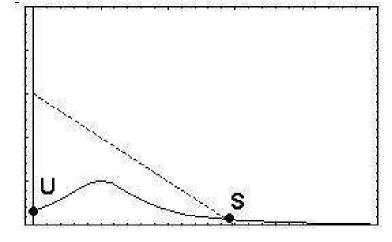
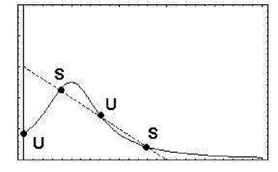
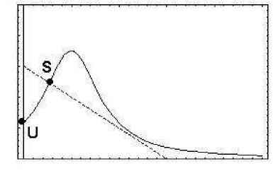
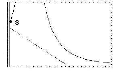
Figure 3: Illustration of the effect of a CIT in an aggressive tumor for increasing values of the CIT.

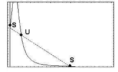
Figure 4: Illustration of the effect of a CIT in an aggressive tumor, similar to figure 3, but with LAS CF coexisting with two other equilibria ($\theta_{cf}$ ”low”).

• Aggressive tumors with variable sign $\Psi^{\prime}(x)$. In such a case, in the absence of therapy there may in the most complex case be one macroscopic equilibrium equilibrium: $E_{Macro}^{o}$ (GAS) and, of course, CF (unstable). Increasing $\theta$ two further equilibria may appear. The analysis is similar to the previous one (cfr figures 3 and 4) and we may find a $\tilde{\theta}$ such that for $\theta>\tilde{\theta}$ CF is GAS. Note that when the tumor is aggressive it is very likely that $\tilde{\theta}$ is ”extremely high”: $\tilde{\theta}>>\sigma$;

• Aggressive tumors with $\Psi^{\prime}(x)<0$ [17]. In such a case, in the absence of therapy there may in the worst case be one macroscopic equilibrium equilibrium: $E_{Macro}^{o}$ (GAS) and, of course, CF (unstable). Increasing $\theta$, if when $y_{I}(0)=y_{c}(0)$ it is $y_{I}^{\prime}(0)<y^{\prime}_{C}(0)$ then we may find two values $\theta_{cf}$ and $\tilde{\theta}>\theta_{cf}$ such that for $\theta_{cf}<\theta<\tilde{\theta}$ $CF$ is LAS and there is the birth of a third unstable equilibrium $E_{u}$. Finally for $\theta>\tilde{\theta}$ CF is GAS. Note that if when $y_{I}(0)=y_{c}(0)$ it is $y_{I}^{\prime}(0)>y^{\prime}_{C}(0)$ then $\theta_{cf}=\tilde{\theta}$.

When $f(0)=+\infty$ the total elimination cannot be achieved by immunotherapy alone. Furthermore, even the suboptimal target of reducing the cancer to a microscopic size in many relevant cases cannot be achieved for therapies of finite duration, however they may be long. In fact, let it be $\Psi(x)>0$ (aggressive tumor) and let there be a unique GAS macroscopic equilibrium $E_{MACRO}$. By applying a CIT with $\theta$ sufficiently high there is a unique GAS microscopic equilibrium. However, when the therapy ceases $\theta$ falls to zero and the cancer restarts growing macroscopically, since $E_{MACRO}$ is again GAS. We note in brief that if the original equilibrium is microscopic (e.g. micrometastasis) the effect of the therapy is simply to create another and temporary microscopic equilibrium.

Let us suppose that there are three co-existing equilibria: $E_{micro}^{o}$ (LAS), $E_{U}^{o}$ (Unstable and through which a separatrix $\Sigma^{o}$ passes) and $E_{MACRO}^{o}$ (LAS). Applying a CIT with $\theta>\tilde{\theta}$ there is an unique GAS microscopic equilibrium. Thus at the end of the therapy (at $t=t_{f}$) depending on the position of $P_{f}=(x(t_{f}),y(t_{f}))$ relatively to $\Sigma^{o}$, we have that either $(x(t),y(t))\rightarrow E_{micro}$ or $(x(t),y(t))\rightarrow E_{MACRO}$.

We note that $\theta$ acts a global bifurcation parameter, and we point out that these behavior may be observed in case of bounded $f(0)$ when therapy is applied for an insufficient time.

Finally, this simple analytical analysis may explain theoretically some numerical results of [15] on the relationships between the efficacy of the cure and the proliferation rate of cancer, and on the correlation between the burden of initial size and the probability of effectiveness of a therapy.

3.3 Periodic Scheduling

In the case of periodic drug schedulings, there is a periodically varying cancer-free solution $CF^{*}=(0,z(t))$, where $z(t)$ is the asymptotic periodic solution of:

$$y^{\prime}=-\Psi(0)y+\sigma+\theta_{m}+\Omega(t)$$ (26)

that, assuming $\Omega(t)=\sum_{n=1}^{+\infty}{C_{k}Cos(k(2\pi/T)t-\zeta_{n})}$, can be rewritten as::

$$z(t)=\frac{\sigma+\theta_{m}}{\Psi(0)}+\sum_{n=1}^{+\infty}{\frac{C_{k}}{\sqrt{\Psi^{2}(0)+k^{2}(\frac{2\pi}{T})^{2}}}Cos(k\frac{2\pi}{T}t-\zeta_{n}-Arg(\Psi(0)+ik\frac{2\pi}{T}))}.$$ (27)

Note that if $T<<1/\Psi(0)$ there is a filtering effect and $z(t)\approx(\sigma+\theta_{m})/\Psi(0)$.

Two basic models of therapy may be:

• $$\theta_{u}(t)=A(1+bcos(\omega t))$$ (28)

  which is rather unrealistic, but whose functional form is commonly used to assess the effect of periodic forcing on nonlinear systems. The asymptotic solution of (26) corresponding to (28) is given by:

  $$z_{u}(t)=\frac{\sigma+A}{\Psi(0)}+\frac{Ab}{\sqrt{\Psi^{2}(0)+\omega^{2}}}Cos(\omega t-Arg(\Psi(0)+i\omega))$$

• the more realistic function:

  $$\theta_{r}(t)=\frac{G}{1-Exp(-cT)}Exp(-cMod(t,T))\textrm{ , }\theta_{m}=\frac{G}{cT},$$ (29)

  which represent a boli-based delivery. The ”shape” of $\theta_{r}(t)$ depends on $c$ and the corresponding asymptotic periodic solution of (26) is given by:

  $$z_{r}(t)=\frac{\sigma}{\Psi(0)}+\frac{G}{\Psi(0)-c}\Big{(}\frac{E^{-cMod(t,T)}}{1-E^{-cT}}-\frac{E^{-\Psi(0)Mod(t,T)}}{1-E^{-\Psi(0)T}}\Big{)}$$

In case of impulsive therapy, by solving the impulsive differential equation

$$y^{\prime}=-\Psi(0)y+\sigma\textrm{, }y(nT^{+})=y(nT^{-})+\gamma\textrm{, }n=0,1,\dots$$ (30)

one obtains that:

$$z(t)=\frac{\sigma}{\Psi(0)}+\frac{\gamma}{1-Exp(-\Psi(0)T)}Exp\Big{(}-\Psi(0)Mod(t,T)\Big{)}.$$ (31)

Furthermore, it is easy to show that the condition $\sigma+\theta_{m}>\sigma_{cr}$ guarantees the LAS of $CF$. In fact, since the variational equations around $(0,z(t))$ are: $U^{\prime}=(\alpha f(0)-\phi(0)z(t))U,W^{\prime}=(\sigma q^{\prime}(0)-\Psi^{\prime}(0)z(t))U-\Psi(0)W$, we obtain that $\alpha f(0)-\phi(0)<z(t)><0\Rightarrow U(t)\rightarrow 0\Rightarrow W(t)\rightarrow 0$, and since $<z(t)>=(\sigma+\theta_{m})/\Psi(0)$ we recover the LAS condition $\sigma+\theta_{m}>\sigma_{cr}$. Similarly, one may demonstrate the GAS condition: $\sigma+\theta_{m}>\sigma^{*}$.

3.4 Numerical simulations

We performed a set of simulations of immunotherapy on the basis of the model proposed by Kuznetsov et al. [14], in which:

$$\alpha f(x)=1.636(1-0.002x),\phi(x)=1,\beta(x)=\frac{1.131x}{20.19+x},\sigma q(x)=0.1181$$

$$\mu(x)=0.00311x+0.3743,$$

and

$$t^{true}=9.9t^{adim}days,(X,Y)=10^{6}(x,y)cells$$

We chose this model since its parameter values were fitted from real data of chimeric mice [14]. Note that the dynamic of tumors in mouse is faster than that of human tumors, and that for periods of about one day or less (i.e. $T<0.101$) it results that $(1/\mu(0))>>T$. Moreover, $\mu^{\prime}(x)=0.00311<<1$ and the tumor is not aggressive. We also performed simulations in a case of a more aggressive tumor, for which we set $\mu(x)=10(0.00311x)+0.3743$. For the non-aggressive tumor $\sigma_{cr}\approx 0.612$ and $\sigma^{*}\approx 1.44>>\sigma$.

It is worth noticing that in other kinds of anticancer therapies the shape of the therapy may be critical in determining whether or not the cancer will be eradicated [8].

In our simulations we assumed $\sigma+\theta_{m}>\sigma_{cr}$ which means that the mean value of the therapy, if given as CIT, would enassure the LAS of the disease free equilibrium. Since for each $T$ the mean value is constant, this means that in the limit $c\rightarrow+\infty$ the therapy $\theta_{r}(t)$ tends to become impulsive.

We found that:

• In the absence of therapy: non-aggressive tumor has two stable equilibria: one slightly less than the carrying capacity and the other corresponding to a small tumor (see phase portrait in figure 5). For the highly aggressive tumor there is one GAS equilibrium slightly less than the carrying capacity;

• With constant therapy: the non-aggressive tumor has a cancer-free equilibrium, which results to be GAS (figure 6). Note that the orbits stemming from initial points characterized by low values of the number of immune system cells are characterized by an initial rapid growth of the tumor size, followed by a regression to $0$. Biologically, the therapy might seem to help the tumor growth, instead of fighting it. For the highly aggressive tumor, the cancer free equilibrium is LAS, but there is also a high size LAS equilibrium (7);

• In the presence of periodic therapy with $\theta_{r}(t)$, for both types of tumors the phase portrait is roughly similar to that of the constant therapy: the cancer-free periodic solution remains GAS for the non aggressive tumor (figure 8). For the aggressive tumor there is the coexistence of the cancer free solution with a solution fluctuating around high values of the cancer size (near the equilibrium of the constant therapy). The two basins of attraction for the aggressive tumor remain unvaried with respect to those of the constant therapy (figure 9).

• For $\theta_{r}(t)$ the dependence of the qualitative properties of the system on the parameter $c$ is not critical.

• For aggressive tumor and $\theta_{u}(t)$, it may occur that, given an initial point, the eradication is also a function of parameters $b$ and $\omega$, but this happens only for unrealistically high values of the therapy period (figure 10), e.g. $T>100$ days. These results may be roughly explained considering that for $T>>Max(1/\Psi(0),1/\alpha)$, one may approximately consider $\theta_{u}(t)$ as constant;

• Both with CIT and with periodic therapy $y(t)$ may reach values considerably higher than the physiological value $\sigma/\mu(0)$, which might model some serious side effects of immunotherapies due to the excess of immunocompetent cells [4, 5].

For the sake of completeness, we also performed some simulations in which $0<A<\sigma_{cr}-\sigma$ and for which there were high oscillations ($b=1$). We obtained the result that for low frequencies, there may be points in the $(\omega,A)$ plane for which eradication is possible. See fig. (11).

Finally, we performed simulations for a hybrid model similar to that by Kuznetsov et al. [14], but in which we assumed:

$$\alpha=0.626,f(x)=Log(\frac{500}{x}),$$

the other parameters being as before. We choose the value $\alpha=0.626$ in order to minimize the difference with $f(x)$ in [14]. The results of the simulations are very close to those relative to the logistic case: figures 12, 13. In order to obtain via CIT the reduction to the microscopic state $\theta>8.4\sigma$ about is required.

The analytical and numerical results obtained in this section may be usefully compared with two similar works of the recent literature which focus on Adoptive Cellular Immunotherapy. An excellent analytical work is [19], who, however, cannot be fully compared with our results because it refers to tumors which have no action in stimulating immune cells. Furthermore, its formulae for the global stability of the cancer free equilibrium are not expressed as a function of the parameters of the therapy. In a very interesting paper [16] some results similar to ours are obtained through numerical bifurcations on a three dimensional model in which the direct immunogenicity of tumors is expressed as an additive term $cx$. As previously stressed, in the absence of therapy and of influx of immunocompetent cells both our model and the model in [16] show the possibility of having periodic solution, which in [16] are shown to be present also in some cases in which there is therapy. We notice in brief that a term $cx$ may be formally embedded in our generic function $\sigma(x)$.

4 Concluding Remarks

It is interesting to use well established conceptual frameworks of ecological models to model competition phenomena in human biology, but it is important to pay attention to the whole ecological modeling aspect, such as the basic requirement of the positivity of the solutions. Even if model [22] violates the positivity rule, it is valuable because it may be read as a model which takes into account a disease-induced depression in the influx of lymphocytes. Then, instead of proposing another specific model, we preferred to add this new feature to a family of equations, and to analyze its properties. We stressed also that models which do not allow the possibility to have LAS tumor-free solutions should be cautiously considered. The general family (8)-(9) may be, of course, further generalized following Volterra’s ecological theory, i.e. by considering that there may be a delay between the consumption of a prey and the birth of a predator (see also [15, 20, 21]), i.e. by allowing a delay $\tau$ with probability density $\varrho(\tau)$. This delayed model and stochastic models will be the subject of further investigations.

Finally, we would like to illustrate some qualitative medical inferences from the investigations that we have here proposed. The main problem of immunotherapy is that, as it is clear from our analysis and simulations, in general, eradication may be possible but is dependent on the initial conditions $(x(0),y(0))$. However, the IC are in medical practice unknown or known with very large confidence intervals (cfr. [59] for the cancer cells at the start of a radiotherapy and). This makes it impossible to plan an anticancer therapy based solely on this therapy. This is a peculiarity of immunotherapy, since there are other kinds of anticancer cures for which a globally stable eradication is possible [8]. However, in our simulations we have seen that in some particular cases the model [14] predicts that globally stable eradication is possible also in case of immunotherapy, but that it depends on the ”degree of aggressiveness” of the cancer, i.e., on the framework of the model [14], on the parameter $\mu_{1}$. However, $\mu_{1}$ is difficult to be estimated (as a range) and, in particular, on single patients. If in the future it might be possible, the option to use immunotherapy as main strategy, for relatively small ”non aggressive” tumors, could be seriously considered. Furthermore, we showed that the behavior of the system does not depend on the amplitude of fluctuations of $\theta(t)$, so that the option of continuous intravenous infusion is not, dynamically, better than the boli based therapy. This result may be of interest, since continuous intravenous infusion may cause major practical problems to the patients. Finally, in case of disease aggressive towards the immune system, since our simulations indicated that all the positive quadrant is GAS towards a macroscopic disease in absence of therapy and low $\sigma$, whereas in the presence of therapy the eradication is possible in an adequate basin (see figure 7), we may infer that a conventional therapy should be followed by immunotherapy to increase the probability of total remission.

5 Acknowledgements

I am very grateful to two anonymous referees who helped me to improve greatly this paper. Special thanks to Prof. Alberto Gandolfi who read the drafts of this papers and gave me precious suggestions, and, for their precious bibliographical help, to Giorgio ”Leppie” Donnini, to William Russell-Edu Esq. and to Matteo ”Furjo” Sisa.

Figure 5: Non aggressive tumor: phase portrait of model [14] in the absence of therapy. There are two LAS equilibria, whose basins of attraction are separated by the separatrix line (plotted with a thick line). The nullcline $y_{C}(x)$ is plotted with short dashes, the nullcline $y_{I}(x)$ and its vertical asymptotes are plotted with long dashes.

Figure 6: Non aggressive tumor: phase portrait of model [14] in the presence of constant therapy with $\sigma+\theta_{m}=1.1\sigma_{cr}$. There is a tumor-free equilibrium $CF=(0,1.799)$, which is globally stable. The nullcline $y_{C}(x)$ is plotted with short dashes, the nullcline $y_{I}(x)$ and its vertical asymptotes are plotted with long dashes. Note that the orbits stemming from initial points characterized by low $y(0)$ are characterized by an initial fast growth of the tumor size, followed by a regression to $0$.

Figure 7: Aggressive tumor: phase portrait of model [14] in presence of constant therapy. There is a tumor-free equilibrium $CF=(0,1.799)$ and another LAS equilibrium, whose basins of attraction are divided by a separatrix line (plotted with a thick line). The nullcline $y_{C}(x)$ is plotted with short dashes, the nullcline $y_{I}(x)$ and its vertical asymptotes are plotted with long dashes.

Figure 8: Non aggressive tumor: phase portrait of model [14] in presence of periodic therapy $\theta_{r}(t)$ with $T=0.202$ (=2 days) and $1/c=0.1T$. There is a tumor free equilibrium $(0,z(t))\approx(0,1.799)$ which remains GAS. The nullcline $y_{C}(x)$ is plotted with short dashing, the nullcline $y_{I}(x)$ and its vertical asymptotes are plotted with long dashes.

Figure 9: Aggressive tumor: phase portrait of the model [14] in the presence of periodic therapy with $T=0.202$ (=2 days) and $1/c=0.5T$. The basins of attraction of the tumor-free equilibrium $CF^{*}=(0,z(t))\approx(0,1.799)$ and of the macroscopic size equilibrium remain near unchanged respect to the CIT scheduling (the basin of CF is slightly greater than in the CIT). The nullcline $y_{C}(x)$ is plotted with short dashing, the nullcline $y_{I}(x)$ and its vertical asymptotes are plotted with long dashes.

Figure 10: Aggressive tumor in the presence of immunotherapy $\theta_{u}(t)$: growth behavior in function of the parameters $(\omega,b)$. Black points correspond to eradication, white points to macroscopic growth. The initial condition for all is $(40,2.5)$ (chosen near the separatrix for the constant therapy). Left: $\sigma+A=1.01\sigma_{cr}$, central: $\sigma+A=1.1\sigma_{cr}$ and right: $\sigma+A=1.25\sigma_{cr}$. Note that the frequencies which do not allow eradication are very low, corresponding to absolutely unrealistic periods for the therapy.

Figure 11: Aggressive tumor in the presence of immunotherapy $\theta_{u}(t)$: growth behavior in function of the parameters $(\omega,A)$ for $b=1$, with $A<\sigma_{cr}-\sigma$. Black points correspond to eradication, white points to macroscopic growth. The initial condition for all is $(40,2.5)$ (chosen near the separatrix for the constant therapy).

Figure 12: Simulation of the modified Kutnetsov model with CIT and $\theta_{m}=0.5\sigma$.

Figure 13: Simulation of the modified Kutnetsov model with periodic therapy, $T=0.202$ (2 days), $1/c=0.5T$ and $\theta_{m}=6\sigma$.

References

- [1] P. Boyle, A. d’Onofrio, P. Maisonneuve, G. Severi, C. Robertson, M. Tubiana and U. Veronesi, Measuring progress against cancer in Europe: has the decline targeted for 2000 come about?, Annals of Oncology, 14, 1312-1325, (2003)
- [2] M. J. Quinn, A. d’Onofrio, B. Moeller, R. Black, C. Martinez-Garcia, H. Moeller, M. Rahu, C. Robertson, L. J. Schouten, C. La Vecchia and P. Boyle,Cancer mortality trends in the EU and acceding countries up to 2015 , Annals of Oncology, 14, 1148-1152, (2003)
- [3] P. Boyle , P. Autier, H. Bartelink, J. Baselga, P. Boffetta, J. Burn, H. J. G. Burns, L. Christensen, L. Denis, M. Dicato, V. Diehl, R. Doll, S. Franceschi, C. R. Gillis, N. Gray, L. Griciute, A. Hackshaw, M. Kasler, M. Kogevinas, S. Kvinnsland, C. La Vecchia, F. Levi, J. G. McVie, P. Maisonneuve, J. M. Martin-Moreno, J. Newton Bishop, F. Oleari, P. Perrin, M. Quinn, M. Richards, U. Ringborg, C. Scully, E. Siracka, H. Storm, M. Tubiana, T. Tursz, U. Veronesi, N. Wald, W. Weber, D. G. Zaridze, W. Zatonski, and H. zur Hausen, European Code Against Cancer and scientific justification: third version (2003), Annals of Oncology, 14, 973-1005, (2003)
- [4] M. Pekham, H. M. Pinedo and U. Veronesi, Oxford Textbook of Oncology, Oxford Medical Publications, Oxford, (1995)
- [5] V. T. de Vito Jr., J. Hellman and S. A. Rosenberg, Cancer: principles and practice of Oncology, J. P. Lippincott, Philadelphia, (1997)
- [6] A. Bertuzzi, A. d’Onofrio, A. Fasano and A. Gandolfi, Regression and Regrowth of Tumour Cords Following Single-Dose Anticancer Treatment, Bulletin of Mathematical Biology, 65, 903-931, (2003)
- [7] T. E. Wheldon, Mathematical Models in Cancer Research, Hilger Publishing, Boston-Philadelphia, (1988)
- [8] A d’Onofrio and A. Gandolfi, Tumour eradication by antiangiogenic therapy: analysis and extensions of the model by Hahnfeldt et al. (1999), Mathematical Biosciences, 191, 159-184, (2004)
- [9] New Applications of Cancer Immunotherapy, S. A. Agarwala (Guest Editor), Seminars in Oncology, Special Issue 29-3 Suppl. 7, (2003)
- [10] I. Bleumer, E. Oosterwijk, P. de Mulder and P. F. Mulders, Immunotherapy for Renal Cell Carcinoma, European Urology, 44, 65-75, (2003)
- [11] C. Marras, C. Mendola, F. G. Legnani and F. di Meco , Immunotherapy and biological modifiers for the treatment of malignant brain tumors, em Current Opinions in Oncology, 15, 204-208, (2003)
- [12] J. M. Kaminski , J. B. Summers, M. B. Ward, M. R. Huber and B. Minev, Immunotherapy and prostate cancer, Cancer Treatment Review, 29, 199-209, (2004)
- [13] N. V. Stepanova, Course of the immune reaction during the development of a malignant tumor, Biophysics, 24, 917-923, (1980)
- [14] V. A. Kuznetsov, I. A. Makalkin, M. A. Taylor and A. S. Perelson. Nonlinear dynamics of immunogenic tumors: Parameter estimation and global bifurcation analysis. Bulletin of Mathematical Biology, 56, 295-321, (1994)
- [15] F. Nani and M. N. Oguztoreli, Modelling and simulation of Rosenberg type adoptive cellular immunotherapy, IMA Journal of Mathematics Applied in Medicine and Biology, 11, 107-147 (1994)
- [16] D. Kirschner, J. C. Panetta, Modeling immunotherapy of the tumor - immune interaction, Journal of Mathematical Biology, 37, 235-252, (1998)
- [17] H. Ortega, Un Modelo Logistico para Crecimiento Tumoral en Presencia de Celulas Asesinas, Revista Mexicana de Ingenieria Biomedica, 20, 61-67, (1999)
- [18] N. Bellomo and L. Preziosi, Modelling and mathematical problems related to tumor evolution and its interaction with the immune system”, Mathematical and Computer Modelling, 32, 413-452, (2000).
- [19] F. Nani and H.I. Freedman, A mathematical model of cancer treatment by immunotherapy , Mathematical Biosciences, 163, 159-199, (2000)
- [20] M. Galach, Dynamics of the tumor-immune system competition: the effect of time delay, International Journal of Applied Mathematics and Computer Science, 13-3, 395-406, (2003)
- [21] S. Szymanska, Analysis of the immunotherapy models in the context of cancer dynamics, International Journal of Applied Mathematics and Computer Science, 13-3, 407-418, (2003)
- [22] O.Sotolongo-Costa, L. Morales-Molina, D. Rodriguez-Perez, J. C. Antonranz and M. Chacon-Reyes, Behavior of tumors under nonstationary therapy, Physica D, 178, 242-253, (2003)
- [23] H. P. de Vladar and J. A. Gonzalez, Dynamic response of cancer under the influence of immunological activity and therapy, Journal of Theoretical Biology, 227, 335-348, (2004)
- [24] N Bellomo, A. Bellouquid and M. Delitala, Mathematical Topics on the Modelling Complex Multicellular Systems and Tumor Immune Cells Competition”, Mathematical Models and Methods in Applied Sciences, 14, 1683-1733, (2004)
- [25] J. Schmielau and O.J. Finn, Activated granulocytes and granulocyte-derived hydrogen peroxide are the underlying mechanism of suppression of T-cell function in advanced cancer patients , Cancer Research, 61, 4756-4760, (2001)
- [26] D. Hart, E. Shochat and Z. Agur, The growth law of primary breast cancer as inferred from mammography screening trials data, British Journal of Cancer, 78, 382-387, (1998)
- [27] C. Guiot, P. G. Degiorgis, P. P. Delsanto, P. Gabriele and T. S. Deisboecke, Does tumor growth follow a universal law ?, Journal of Theoretical Biology, 225, 147-151 ,(2003)
- [28] A. Bru, S. Albertos, J.L. Subiza, J.L. Garcia-Asenjo and I. Bru, The Universal Dynamics of Tumor Growth, Biophysical Journal, 85, 2948-2961, (2003)
- [29] B J Kennedy, Cyclic leukocyte oscillations in chronic myelogenous leukemia during hydroxyurea therapy, Blood, 35, 751-760, (1970)
- [30] H Vodopick, E.M. Rupp, C. L. Edwards, F.A. Goswitz and J.J. Beauchamp, Spontaneous cyclic leukocytosis and thrombocytosis in chronic granulocytic leukemia , The New England Journal of Medicine, 286, 284-290, (1972)
- [31] H. Tsao, A. B. Cosimi and A. J. Sober, Ultra-late recurrence (15 years or longer) of cutaneous melanoma, Cancer, 79, 2361-2370, (1997)
- [32] G. Bonadonna, G. Robustelli della Cuna (Eds.), Medicina Oncologica, Masson, Milano, 259-272, (1994)
- [33] A. Kane Laird, Dynamics of tumor growth, British Journal of Cancer, 18, 490-502, (1964)
- [34] A. Kane Laird, Dynamics of tumor growth: comparison of growth rates and extrapolation of growth curve to one cell, British Journal of Cancer, 19, 278-290, (1965)
- [35] I.D. Bassukas, Gompertzian re-evaluation of the growth patterns of transplantable mammary tumours in sialoadenectomized mice, Cell Proliferation, 27, 201-211, (1994)
- [36] N. Olea, M. Villalobos, M.I. Nunez, J. Elvira, J.M. Ruiz de Almodovar, Evaluation of the growth rate of MCF-7 breast cancer multicellular spheroids using three mathematical models, Cell Proliferation, 27, 213-227, (1994)
- [37] A.M. Parfitt, Gompertzian growth curves in parathyroid tumours: further evidence for the set-point hypothesis, Cell Proliferation, 30, 341-649, (1994)
- [38] K. Rygaard, M. Spang-Thomsen, Quantitation and Gompertzian analysis of tumor growth, Breast Cancer Research and Treatment, 46, 303-312, (1997)
- [39] A.M. Ballangrud, W.H. Yang, A. Dnistrian, N.L. Lampen and G. Sgourous , Growth anc characterization of LNCaP Prostate Cancer, Clinical Cancer Research, 5, 3171s-3167s, (1999)
- [40] D.A. Cameron, The relative importance of proliferation and cell death in breast cancer growth and response to tamoxifen , European Journal of Cancer, 37, 1545-1553, (2001)
- [41] M.A.A. Castro, F. Klamt, V.A. Grieneisen, I. Grivicich and J.C.F. Moreira , Gompertzian growth pattern correlated with phenotypic organization of colon carcinoma, malignant glioma and non-small cell lung carcinoma cell lines, Cell Proliferation, 36, 65-73, (2003)
- [42] M. Gyllenberg and G. Webb, Quiescence as an explanation of Gompertzian tumor growth, Growth, Development and Aging,53, 25-33 (1989)
- [43] C, Calderon and T. Kwembe, Modeling Tumor Growth, Mathematical Biosciences, 103, 97-114 (1991)
- [44] E.K. Afenya, C.P. Calderon, Diverse ideas on the growth kinetics of disseminated cancer cells, Bulletin of Mathematical Biology , 62, 527-542, (2000)
- [45] E.K. Afenya, C.P. Calderon, Growth kinetics of cancer cells prior to detection and treatment: an alternative view, Discrete and Continuous Dynamical Systems - B, 5, 25-28, (2004)
- [46] M. Molski and J. Konarski, Coherent states of Gompertzian growth , Physical Review E, 68 Art. No. 021916 Part 1 AUG (2003)
- [47] P. Waliszewski and J. Konarski, The Gompertzian curve reveals fractal properties of tumor growth, Chaos Solitons and Fractals, 16, 665-674, (2003)
- [48] P. Castorina and D. Zappala’, Tumor Gompertzian growth by cellular energetic balance, arXiv:q-bio.CB/0407018 v2 21 Dec 2004
- [49] P. Castorina and D. Zappala’, Energetic Model of Tumor Growth, arXiv:q-bio.TO/0412040 v1 22 Dec 2004
- [50] M. Marusic, Z. Bajzer, J. P. Freyer and S. Vuk-Pavlovic, Analysis of growth of multicellular tumour spheroids by mathematical models, Cell Proliferation, 27, 73-94, (1994)
- [51] I.M. van Leeuwen and C. Zonneveld, From exposure to effect: a comparison of modeling approaches to chemical carcinogenesis, Mutation Research, 489, 17-45, (2001)
- [52] R. Demicheli, R. Foroni, A. Ingrosso, G. Pratesi, C. Soranzo and M. Tortoreto, An Exponential-Gompertzian Description of LoVo Cell Tumor Growth from in Vivo and in Vitro Data, Cancer Research, 49, 6543-6546, (1989)
- [53] V.G. Vaydia and F.J. Alexandro Jr, Evaluation of some mathematical models for tumor growth, International Journal of Biomedical Computation, 13, 19-36, (1982)
- [54] G. G. Steel, Groth Kinetics of Tumours, Clarendon Press, Oxford, (1977)
- [55] S. Piantadosi, A Model of Growth with first-order birth and death rates, Computers and biomedical research, 18, 220-232, (1985)
- [56] H Thieme, Mathematics in population biology, Princeton University Press, Princeton, (2003)
- [57] G.P. Dunn, A.T. Bruce, H. Ikeda, L.J. Old and R. D. Schreiber, Cancer immunoediting: from immunosurveillance to tumor escape, Nature Immunology, 3, 991-997, (2002)
- [58] G.P. Dunn, L.J. Old and R. D. Schreiber, The three ES of Cancer Immunoediting, Annual Review of Immunology, 22, 322-360, (2004)
- [59] F.M.O. Al-Dwery, D. Guirado, A.M. Lallena and V. Pedraza, Effect of tumour control of time interval between surgery and postoperative radiotherapy: an empirical approach using Monte Carlo simulation, Physics in Medicine and Biology, 49, 2827-2839, (2004)