Thermal screening at finite chemical potential on a topological surface and its interplay with proximity-induced ferromagnetism

Abstract

Motivated by recent experiments on EuS/Bi₂Se₃ heterostructures, we study the temperature dependent screening effects on the surface of a three-dimensional topological insulator proximate to a ferromagnetically ordered system. In general, we find that besides the chemical potential and temperature, the screening energy scale also depends on the proximity-induced electronic gap in an essential way. In particular, at zero temperature the screening energy vanishes if the chemical potential is smaller than the proximity-induced electronic gap. We show that at finite temperature, $T$, and/or chemical potential, $\mu$, the Chern-Simons (topological) mass, which is generated by quantum fluctuations arising from the proximity-effect, can be calculated analytically in the insulating regime. In this case the topological mass yields the Hall conductivity associated to edge states. We show that when the chemical potential is inside the gap the topological mass remains nearly quantized at finite temperature.

I Introduction

Recently three-dimensional topological insulators (TIs) with magnetically ordered surface states had attracted much attention, both theoretically Nagaosa-2010 ; Nagaosa-2010-1 ; Zang-Nagaosa ; Franz-2010 ; Rosenberg-2010 ; Belzig-2012 ; Loss-PRL-2012 ; Nogueira-Eremin-2012 ; Cortijo-2012 ; Schmidt-2012 ; Qi-2013 ; Chulkov and experimentally.Hor ; Wray ; Vobornik ; Rader-2012 ; Checkelsky ; Moodera-2012 ; Moodera ; kapitulnik-2013 The topological surface states, usually gapless and featuring a low-energy Dirac dispersion protected by time-reversal (TR) symmetry, generally become gapped when a ferromagnetically ordered layered material is grown over it. In this case the TR symmetry is broken by the proximity effect to the magnetic material. Interesting effects on the magnetization dynamics arise when the topological surface becomes ferromagnetic.Nagaosa-2010 ; Franz-2010 ; Loss-PRL-2012 ; Nogueira-Eremin-2012 Quantum fluctuations of the surface Dirac fermions induce an additional Berry phase, which modifies the Landau-Lifshitz (LL) equation for the magnetization dynamics.Nagaosa-2010 ; Nogueira-Eremin-2012 Furthermore, when an electric field is present, either external or originating from Coulomb interactions, a topological magnetoelectric torque also appears in the LL equation.Nogueira-Eremin-2012 Actually both effects arise from an induced Chern-Simons (CS) term CS upon integrating out the Dirac fermions.Nogueira-Eremin-2012 ; Nogueira-Eremin-2013

It is important to notice that most of the theoretical calculations in TIs were performed so far only at zero temperature, although some aspects like the shift of the Curie temperature in the ferromagnetic insulator/TI heterostructure were discussed.Nogueira-Eremin-2012 ; Moodera The disregard of the temperature effects till now is partially connected to the fact that finite temperature is not expected to modify the topological contribution to the effective electromagnetic Lagrangian of a TI in the bulk,Qi-2008

$${\cal L}_{\rm EM}=\frac{1}{8\pi}\left(\epsilon{\bf E}^{2}-\frac{1}{\mu_{0}}{\bf B}^{2}\right)+\frac{\alpha}{4\pi^{2}}\theta~{}{\bf E}\cdot{\bf B},$$ (1)

where $\alpha=e^{2}/(\hbar c)$ is the fine-structure constant and $\theta$ is the so-called axion field Axions . While both the dielectric constant, $\epsilon$, and magnetic permeability, $\mu_{0}$, receive finite temperature corrections, $\theta$ remains temperature-independent.Liu-Ni-PRD-1988 This somewhat confirms the naive expectation for the term being topological in origin. This, however, is not the full story. For example, differently from the chiral anomaly leading to the axion term in Eq. (1), the parity anomaly in $d=2+1$ dimensions does indeed receive finite temperature corrections.CS-finite-T Therefore, integrating out the Dirac fermions in 2+1 dimensions and at finite temperature generates additional temperature-dependent CS term.

Another important finite temperature aspect relates to the electromagnetic response and the many-body screening of the Coulomb interaction. In graphene, where the chemical potential is typically zero, there is no screening of the long-range Coulomb interaction at zero temperature, although a renormalization of the dielectric constant occurs.interac-graphene However, at finite temperature a thermal screening should occur, corresponding to a situation reminiscent of massless QED in $2+1$ dimensions.Dorey-1991 Moreover, in contrast to graphene, most three-dimensional TIs feature surface Dirac fermions at a non-vanishing chemical potential, and we may expect that the screening in TIs Zang-Nagaosa ; Screen-TI and in doped graphene Ando-2006 at zero temperature behaves differently.

In recent experiments Moodera ; kapitulnik-2013 thin films of EuS/Bi₂Se₃ heterostructure were grown, and it has been shown that the topological surface becomes ferromagnetic due to a proximity-induced symmetry breaking mechanism. The experiments also confirmed the theoretical expectations that the surface Dirac fermions become gapped.Moodera ; kapitulnik-2013 Many measurements in such a heterostructure are made at temperatures close to the Curie temperature. Therefore, it is of paramount importance to study theoretically quantum field theory models of Dirac fermions at finite temperature and chemical potential. As we have mentioned above, there are finite temperature corrections to the generated CS term. Furthermore, since the CS term provides a correction to the Berry phase of the proximity-induced ferromagnetism,Nagaosa-2010 ; Nogueira-Eremin-2012 the precessional behavior of the magnetization will be modified at finite temperature and in turn affect the spin-wave excitations.

A finite chemical potential influences the physics on the surface dramatically even at zero temperature. For example, it is known that when the chemical potential is larger than the gap, the Hall conductivity is not quantized any longer and is given by Zang-Nagaosa $\sigma_{xy}=e^{2}m_{0}/(2h\mu)$. Here $m_{0}$ represents the zero temperature gap. This suggests that in such a metallic regime the Hall conductivity cannot always be identified with the coefficient of a local fluctuation-generated CS term, i.e., the topological mass which is induced by quantum fluctuations rather than by an external response. Since the relevant situation for the magnetization dynamics is when the chemical potential is inside the gap, it is important to ask whether the Hall conductivity remains quantized in this case when the temperature is finite. In this paper we will derive an analytical expression for Hall conductivity at finite temperature and chemical potential in precisely this regime. We will show that a plateau persists at finite temperature when the chemical potential is inside the gap.

The plan of the paper is as follows. In Section II we introduce the model and discuss some simple thermally induced screening effects following from the vacuum polarization on the TI surface. In Section III we derive the low-energy CS term at finite temperature and chemical potential. We discuss the physical consequences of this result for the magnetization dynamics in Section IV, and in Section V we summarize the main results.

II Model and vacuum polarization at finite temperature

Our starting point is the following Hamiltonian for the surface Dirac fermions, $H=\psi^{\dagger}{\cal H}~{}\psi$, where $\psi=[\psi_{\uparrow},\psi_{\downarrow}]^{T}$. The $2\times 2$ matrix ${\cal H}$ reads,

$${\cal H}=v_{F}(-i\hbar{\mbox{\boldmath$\nabla$}}\times\hat{\bf z})\cdot{{\mbox{\boldmath$\sigma$}}}-e\varphi-J(n_{x}\sigma_{x}+n_{y}\sigma_{y})-J_{\perp}n_{z}\sigma_{z},$$ (2)

where $\varphi$ is a scalar potential including contributions both from external electric field and Coulomb interaction, and the magnetization ${\bf n}$ satisfies the constraint ${\bf n}^{2}=1$. The Lagrangian ${\cal L}=\psi^{\dagger}i\hbar\partial_{t}\psi-H$ can be after a rescaling $\varphi\to(J/e)\varphi$ conveniently written in QED-like form,Nogueira-Eremin-2012 ; Nogueira-Eremin-2013

$${\cal L}=\bar{\psi}(i\hbox to0.0pt{\hbox to5.30904pt{\hfil/\hfil}\hss}\partial-J\hbox to0.0pt{\hbox to5.28589pt{\hfil/\hfil}\hss}a-J_{\perp}n_{z})\psi,$$ (3)

In the above equation the Dirac slash notation is used, $\hbox to0.0pt{\hbox to7.90555pt{\hfil/\hfil}\hss}Q=\gamma^{\mu}Q_{\mu}$, with $\gamma^{0}=\sigma_{z}$, $\gamma^{1}=-i\sigma_{x}$, and $\gamma^{2}=i\sigma_{y}$, and $\partial_{\mu}=\hbar(\partial_{t},v_{F}{\mbox{\boldmath$\nabla$}})$, $\bar{\psi}=\psi^{\dagger}\gamma^{0}$, and the vector field $a^{\mu}=(a_{0},{\bf a})=(\varphi,n_{y},-n_{x})$.

In order to study thermal effects on the magnetization dynamics and the screening of the Coulomb interaction, we will perform the calculations in the imaginary time formalism, setting as usual $t=-i\tau$ with $\tau\in[0,\beta]$, and integrating out the fermions with anti-periodic boundary conditions, $\psi(0,{\bf r})=-\psi(\beta,{\bf r})$. Thus, the amplitude $\exp(i\hbar^{-1}\int d^{3}x{\cal L}_{F})$ appearing in the functional integral becomes $\exp(-\hbar^{-1}\int_{0}^{\beta}d\tau\int d^{2}r{\cal L}_{F}^{\rm eucl})$ in the imaginary time formalism, with the Lagrangian in euclidean spacetime given by,

$${\cal L}^{\rm eucl}=\bar{\psi}(\hbox to0.0pt{\hbox to5.30904pt{\hfil/\hfil}\hss}\partial-\mu\gamma_{0}-iJ\hbox to0.0pt{\hbox to5.28589pt{\hfil/\hfil}\hss}a+J_{\perp}n_{z})\psi,$$ (4)

where now the Dirac slash features the euclidean Dirac matrices $\gamma_{\mu}=(\sigma_{z},\sigma_{x},-\sigma_{y})$ and a chemical potential $\mu$ was included (note that $\psi^{\dagger}\psi=\bar{\psi}\gamma_{0}\psi$). Integrating out the fermions yields the effective action in the form, ${\cal S}_{\rm eff}={\cal S}_{F}+{\cal S}_{\rm mag}({\bf n})$, with

$${\cal S}_{F}=-\frac{N}{V}{\rm Tr}\ln(\hbox to0.0pt{\hbox to5.30904pt{\hfil/\hfil}\hss}\partial-\mu\gamma_{0}-iJ\hbox to0.0pt{\hbox to5.28589pt{\hfil/\hfil}\hss}a+J_{\perp}n_{z}),$$ (5)

where $N$ is the number of Dirac fermion species and $V$ is the (infinite) volume. ${\cal S}_{\rm mag}({\bf n})$ is the magnetic action, which has the general form in the imaginary time formalism,

$${\cal S}_{\rm mag}=\int d\tau\int d^{2}r\left[{\bf b}({\bf n})\cdot\partial_{\tau}{\bf n}+{\cal H}_{\rm mag}\right],$$ (6)

featuring a Berry gauge potential satisfying ${\mbox{\boldmath$\nabla$}}_{\bf n}\times{\bf b}={\bf n}$, representing a magnetic monopole in the magnetization space. The magnetic Hamiltonian density ${\cal H}_{\rm mag}$ may contain several contributions, the most important ones being the coupling to external fields and the exchange terms.

In TIs the number $N$ of fermion species is odd. In the present context this is essential, otherwise no parity and TR symmetry breaking via the generation of a CS term would occur dynamically.Nogueira-Eremin-2013 Assuming that the system orders along the $z$-axis, we can write $n_{z}=\langle n_{z}\rangle+\tilde{n}_{z}$ and expand Eq. (5) up to quadratic order in the fields,

$${\cal S}_{F}\approx\frac{N}{2}\int_{0}^{\beta}d\tau\int d^{2}r\int_{0}^{\beta}d\tau^{\prime}\int d^{2}r^{\prime}\left[\Pi_{\mu\nu}(\tau-\tau^{\prime},{\bf r}-{\bf r}^{\prime})\right.$$ (7)

$$\times \left.a_{\mu}(\tau,{\bf r})a_{\nu}(\tau^{\prime},{\bf r}^{\prime})+\chi_{zz}(\tau-\tau^{\prime},{\bf r}-{\bf r}^{\prime})\tilde{n}_{z}(\tau,{\bf r})\tilde{n}_{z}(\tau^{\prime},{\bf r}^{\prime})\right],$$

where $\Pi_{\mu\nu}(\tau-\tau^{\prime},{\bf r}-{\bf r}^{\prime})=\delta^{2}{\cal S}_{F}/[\delta a_{\mu}(\tau,{\bf r})\delta a_{\nu}(\tau^{\prime},{\bf r}^{\prime})]|_{n_{z}=\langle n_{z}\rangle}$, is the vacuum polarization tensor at finite temperature encompassing screening effects in the Coulomb potential and the transverse magnetic susceptibility, and $\chi_{zz}(\tau-\tau^{\prime},{\bf r}-{\bf r}^{\prime})=\delta^{2}{\cal S}_{F}/[\delta\tilde{n}_{z}(\tau,{\bf r})\delta\tilde{n}_{z}(\tau^{\prime},{\bf r}^{\prime})]|_{n_{z}=\langle n_{z}\rangle}$, is the longitudinal magnetic susceptibility. The fermionic propagator has the form, $G_{F}=(\hbox to0.0pt{\hbox to5.30904pt{\hfil/\hfil}\hss}\partial-\mu\gamma_{0}+m)^{-1}$, or in momentum space, $G_{F}(p)=(i\hbox to0.0pt{\hbox to5.03125pt{\hfil/\hfil}\hss}p+\mu\gamma_{0}+m)^{-1}=[m-(i\omega_{n}+\mu)\gamma_{0}-i{\mbox{\boldmath$\gamma$}}\cdot{\bf p}]/[m^{2}+{\bf p}^{2}-(i\omega_{n}+\mu)^{2}]$, where $p=(p_{\mu})=(p_{0},{\bf p})=(\omega_{n},v_{F}{\bf k})$, $m=J_{\perp}\langle n_{z}\rangle$, and $\omega_{n}=(2n+1)\pi/\beta$ is the usual fermionic Matsubara frequency. The units are such that $\hbar=1$.

The calculation of the vacuum polarization in $2+1$ dimensions and zero temperature is well known CS and has been reviewed by us in detail recently in Ref. Nogueira-Eremin-2013, . Due to current conservation, it fulfills $p_{\mu}\Pi_{\mu\nu}=0$. Periodicity in the Matsubara time allows one to choose a rest frame for the heat bath given by the vector $u_{\mu}=(1,0,0)$.Kapusta Therefore, in this case we can write the vacuum polarization in momentum space in the form,

$$\Pi_{\mu\nu}(p)=A(p)P_{\mu\nu}^{T}+B(p)P_{\mu\nu}^{L}+C(p)\epsilon_{\mu\nu\lambda}p_{\lambda},$$ (8)

where $P_{\mu\nu}^{T}$ and $P_{\mu\nu}^{L}$ are both transverse in 2+1 dimensions, with $P_{\mu\nu}^{T}$ being transverse and $P_{\mu\nu}^{L}$ longitudinal in two spatial dimensions. Thus, we have $P_{0i}^{T}=P_{00}^{T}=0$, $P_{ij}^{T}=\delta_{ij}-p_{i}p_{j}/{\bf p}^{2}$, and $P_{\mu\nu}^{T}+P_{\mu\nu}^{L}=\delta_{\mu\nu}-p_{\mu}p_{\nu}/p^{2}$, where Latin indices refer to spatial dimensions. At the same time,

$$\Pi_{\mu\nu}(\omega_{n},{\bf p})=-NJ^{2}T$$ (9)

$$\times \sum_{l}\int\frac{d^{2}k}{(2\pi)^{2}}{\rm tr}[\gamma_{\mu}G_{F}(\nu_{l},{\bf k})\gamma_{\nu}G_{F}(\nu_{l}+\omega_{n},{\bf k}+{\bf p})],$$

where $\nu_{l}=\pi(2l+1)T$ and $\omega_{n}=2\pi nT$, $l,n\in\mathbb{Z}$.

At finite temperatures, an interesting aspect of the vacuum polarization in relativistic-like fermionic systems is the generation of a thermal mass for the vector field along the time direction.Kapusta ; Dorey-1991 In other words, the Coulomb potential acquires a thermal gap or thermal screening. In the case of a TI surface, for example, the Coulomb interaction $\phi_{C}(r)=e^{2}/(\epsilon r)$ in momentum space is given by $\phi_{C}({\bf q})=2\pi e^{2}/(\epsilon|{\bf q}|)$, similarly to interacting graphene.interac-graphene The vacuum polarization screens this Coulomb interaction, and we have, $\phi_{\rm eff}({\bf q})=J^{2}/\{J^{2}[\phi_{c}({\bf q})]^{-1}+\Pi_{00}(0,{\bf q})\}$, allowing us to define the so called electric mass,Kapusta $m_{\rm el}^{2}\equiv\Pi_{00}(0,0)$. An explicit calculation assuming $|{\bf q}|\ll\sqrt{2(\mu^{2}-m^{2})}$ yields,

$$\Pi_{00}(0,{\bf q})=\frac{NJ^{2}}{2\pi v_{F}^{2}}\left\{T\ln[\cosh(|m|/T)+\cosh(\mu/T)]-\frac{{\bf q}^{2}+2m^{2}}{\sqrt{{\bf q}^{2}+4m^{2}}}\frac{\sinh\left(\frac{\sqrt{{\bf q}^{2}+4m^{2}}}{2T}\right)}{\cosh(\mu/T)+\cosh\left(\frac{\sqrt{{\bf q}^{2}+4m^{2}}}{2T}\right)}\right\},$$ (10)

so that the electric mass is given by,

$$m^{2}_{\rm el} = \frac{NJ^{2}}{2\pi v_{F}^{2}}\left\{\vphantom{\frac{1}{2}}T\ln[\cosh(|m|/T)+\cosh(\mu/T)]\right.$$ (11)

$$- \left.\frac{|m|\sinh(|m|/T)}{\cosh(|m|/T)+\cosh(\mu/T)}\right\}.$$

At zero temperature, $m_{\rm el}^{2}|_{T=0}=[NJ^{2}\mu/(2\pi v_{F}^{2})]\theta(\mu-|m_{0}|)$, where $m_{0}=\lim_{T\to 0}m(T)$. Thus, the electric mass vanishes for $0\leq\mu<|m_{0}|$. Using the above results, we obtain that in the long wavelength limit the effective Coulomb interaction becomes,

$$\phi_{\rm eff}({\bf q})\approx\frac{J^{2}}{J^{2}[\phi_{c}({\bf q})]^{-1}+\Pi_{00}(0,0)}=\frac{2\pi e^{2}}{\epsilon(|{\bf q}|+s)},$$ (12)

where $s=2\pi e^{2}m_{\rm el}^{2}/(\epsilon J^{2})$, featuring in this way a screening of the Thomas-Fermi type. At zero temperature, $s|_{T=0}\equiv s_{0}=Ne^{2}\mu\theta(\mu-|m_{0}|)/(\epsilon v_{F}^{2})$. In real space we have,

$$\phi_{\rm eff}(r)=\frac{e^{2}}{\epsilon r}\{1+(\pi sr/2)[Y_{0}(sr)-H_{0}(sr)]\},$$ (13)

where $Y_{0}(x)$ is a Bessel function of second kind and $H_{0}(x)$ is a Struve function.

The above results imply that no screening would occur at zero temperature if $\mu<|m_{0}|=J_{\perp}|\langle n_{z}\rangle|$, i.e., the screening takes place only when the chemical potential is located above the gap. This is a reasonable result, since this regime corresponds to a metallic state.

For temperatures above the Curie temperature, $T_{c}$, we have,

$$s|_{T\geq T_{c}}=\frac{Ne^{2}}{\epsilon v_{F}^{2}}T\ln\left[2\cosh^{2}\left(\frac{\mu}{2T}\right)\right].$$ (14)

The above equation is also valid when no ferromagnetic material is in contact with the TI surface. In this case Eq. (14) is valid for all $T\geq 0$. Interestingly, since we are dealing with interacting Dirac fermions, we have that in absence of ferromagnetism Eq. (14) would also apply to doped graphene Ando-2006 if one replaces $N\to N/2$ to account for the even number of Dirac cones.

III The Chern-Simons term and the Hall conductivity at finite temperature

Next, we consider the finite temperature behavior of the CS term, which will yield a finite temperature correction to the Berry phase on the TI surface. The finite temperature behavior of the CS term is generally a highly nontrivial matter,CS-finite-T ; Dunne-1997 depending on the type of background field configuration involved. However, in our case we are mainly interested in the low-energy behavior, so that the calculation simplifies considerably. The calculation parallels the zero temperature one,Nogueira-Eremin-2013 and thus $C(p)=-2NJ^{2}mI(p)$, where

$$I(\omega_{n},{\bf p}) = T\sum_{l}\int\frac{d^{2}k}{(2\pi)^{2}}\frac{1}{(i\nu_{l}+\mu)^{2}-v_{F}^{2}{\bf k}^{2}-m^{2}}$$ (15)

$$\times \frac{1}{(i\nu_{l}+i\omega_{n}+\mu)^{2}-v_{F}^{2}({\bf k}-{\bf p})^{2}-m^{2}}.$$

When the chemical potential is inside the gap, i.e., $\mu<|m|$, the surface state is insulating and we can take $I(p)\approx I(0)$ in the low-energy regime, since in this case $m$ yields the dominant energy scale in the problem and there is no Fermi momentum. The effective action is local in this case, following straightforwardly from a derivative expansion. On the other hand, in the metallic regime where $\mu>|m|$, the effective action is inherently non-local. In this case there is a Fermi surface singularity with a Fermi momentum $p_{F}=\sqrt{\mu^{2}-m^{2}}$.

Generally, the coefficient of the CS term, the so called topological mass, yields a measure of the Hall conductivity, when scaled in appropriate unities. We will now show that in the insulating regime, the topological mass can be evaluated analytically at finite temperature and chemical potential. In this regime the CS contribution to the effective action is given approximately by,

$${\cal S}_{\rm CS}\approx\frac{\sigma(T,m)}{2}\int dt\int d^{2}r\epsilon_{\mu\nu\lambda}a^{\mu}\partial^{\nu}a^{\lambda}$$ (16)

where in the above expression we have returned to real time and have defined $\sigma(T,m)=2NJ^{2}I(0)m$. Expressing $\sigma(T,m)$ in units of conductivity via $\sigma(T,m)=NJ^{2}\tilde{\sigma}(T,m)/(v_{F}^{2}e^{2})$ and using that $I(0)=[f_{-}(0)-f_{+}(0)]/(8\pi|m|)$ (see appendix A), we obtain,

$$\tilde{\sigma}(T,m)=\frac{e^{2}{\rm sgn}(m)\sinh(|m|/T)}{2h[\cosh(|m|/T)+\cosh(\mu/T)]},$$ (17)

where we have reintroduced the Planck constant. The above equation provides an analytical expression for the Hall conductivity for the case where the chemical potential is inside the gap, i.e., in the insulating regime. However, it differs from the actual Hall conductivity $\sigma_{xy}$ when $\mu>m$. In order to see this, let us first compare Eq. (17) to the Hall conductivity at zero temperature, where it can be calculated exactly for a nonzero chemical potential.

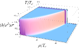
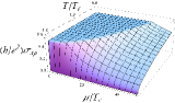
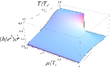
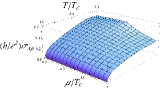
Figure 1: Calculated topological mass $\tilde{\sigma}(T,m)$ and Hall conductivity $\sigma_{xy}$ as a function of temperature, $T$, and the chemical potential, $\mu$, normalized by the Curie temperature $T_{c}$. We consider for $m(T)$ a mean-field temperature dependence, $m(T)\approx J_{\perp}\sqrt{1-T/T_{c}}$ and use the estimate $J_{\perp}/T_{c}\approx 37.4$ [(a) and (b)] based on experimental results from Ref. Moodera, for the Bi₂Se₃/EuS interface. Note the plateau regions in both panels (a) and (b), indicating nearly quantized $\tilde{\sigma}$ and $\sigma_{xy}$, although both $T$ and $\mu$ are finite. There is a large region in the $T-\mu$ plane where the Hall conductivity is finite and not quantized, while the topological mass vanishes. Panels (a) and (b) depict a situation where $J_{\perp}$ is large compared to $T_{c}$. In panels (c) and (d) we illustrate a situation with $J_{\perp}/T_{c}=0.8$. Observe that the region of the plateau is smaller and less sharp. In any situation, the plot of the topological mass represents the Hall conductivity only in the regime $\mu<|m|$.

Introducing the unit vector $\hat{d}(k)={\bf d}(k)/|{\bf d}(k)|$ associated to the mean-field Hamiltonian ${\cal H}_{\rm MF}={\bf d}(k)\cdot{\mbox{\boldmath$\sigma$}}=-k_{y}\sigma_{x}+k_{x}\sigma_{y}+m\sigma_{z}$, we can write an expression for $\sigma_{xy}(T,m)$ in terms of the topological charge density,

$${\cal Q}_{xy}(k)=\frac{1}{2\pi}\hat{d}(k)\cdot[\partial_{k_{x}}\hat{d}(k)\times\partial_{k_{y}}\hat{d}(k)].$$ (18)

as

$$\sigma_{xy}(T,m)=\frac{e^{2}}{2h}\int d^{2}k~{}{\cal Q}_{xy}(k)[f_{-}(k)-f_{+}(k)],$$ (19)

where $f_{\pm}(k)=1/[e^{\beta(\pm|{\bf d}(k)|-\mu)}+1]$ are Fermi-Dirac distributions. Thus, it is straightforward to compute $\sigma_{xy}$ at $T=0$, Zang-Nagaosa

$$\sigma_{xy}(0,m_{0})=\frac{e^{2}}{2h}\left[\left({\rm sgn}(m_{0})-\frac{m_{0}}{\mu}\right)\theta(|m_{0}|-\mu)+\frac{m_{0}}{\mu}\right],$$ (20)

and we see that the Hall conductivity at $T=0$ is non-quantized and non-universal in the metallic regime ($\mu>m_{0}$). The topological mass, on the other hand, vanishes in the limit $T\to 0$ when $\mu>|m_{0}|$,

$$\tilde{\sigma}(0,m_{0})=\frac{e^{2}}{2h}{\rm sgn}(m_{0})\theta(|m_{0}|-\mu).$$ (21)

Thus, when the system is in the metallic phase, the topological mass obtained from the low-energy regime of the CS action does not agree with the Hall conductivity. This means that non-local corrections have to be considered in order to make the local effective action approach to agree with the expression obtained from linear response. Further insight on this point is obtained by considering how the topological mass relates to the actual Hall conductivity and see how it deviates from it in the metallic regime. First, we note that we can write,

$$\tilde{\sigma}(T,m)=\sigma_{xy}(T,m)+\tau_{xy}(T,m),$$ (22)

where

$$\tau_{xy}(T,m)=-\frac{e^{2}}{2h}\int d^{2}k~{}{\cal Q}_{xy}(k)|{\bf d}(k)|\frac{\partial}{\partial\mu}[f_{+}(k)+f_{-}(k)],$$ (23)

The quantity $\tau_{xy}$ yields the deviation of the coefficient of the local contribution to the CS term from the Hall conductivity when the chemical is above the gap. We see that for $|m_{0}|<\mu$ the contribution $\tau_{xy}$ is responsible for canceling the non-quantized contribution at $T=0$, since,

$$\tau_{xy}(T=0) = -\frac{e^{2}}{2h}\int d^{2}kQ_{xy}(k)|{\bf d}(k)|\delta(|{\bf d}(k)|-\mu)$$ (24)

$$= -\frac{e^{2}m_{0}}{2h\mu}=-\sigma_{xy}(T=0,|m_{0}|<\mu),$$

precisely canceling the last term in Eq. (20). Thus, we see that the chemical potential acts as a cutoff setting the limit of validity of the local effective action.

In Fig. 1(a) we show $\tilde{\sigma}(T,m)$ for a typical mean-field theory dependence with the temperature for $m$. In order to plot $\tilde{\sigma}$ and $\sigma_{xy}$ we have used values for $J_{\perp}$ and Curie temperature estimated from the experiment by Wei et al. Moodera performed on Bi₂Se₃/EuS samples. There the estimated value for $J_{\perp}$ at the interface is considerably larger ($\sim 150$ meV private ) than the one obtained in ab initio calculations for Bi₂Se₃/MnSe,Qi-2013 ; Chulkov which features an antiferromagnet material (MnSe) rather than a ferromagnetic one.

The numerical calculation of the Hall conductivity is shown in Fig. 1(b). We note a plateau similar to the one arising for $\tilde{\sigma}$, which indicates that quantization nearly holds for finite $T$ and $\mu$ in a region of the $T-\mu$ plane determined by the inequality $\mu<|m(T)|$. However, there is also a region in the $T-\mu$ plane where the Hall conductivity is non-quantized while the topological mass $\tilde{\sigma}$ vanishes.

Note that sharp and large plateau regions up to $T=T_{c}$ [Fig. 1, panels (a) and (b)] occur only if the gap is larger than $T_{c}$, which is precisely the case in the experiment from Ref. Moodera, . In panels (c) and (d) of Fig. 1 we also illustrate the opposite situation, taking for example, $J_{\perp}/T_{c}=0.8$. Observe that the plateau region here is not as sharp and loses its approximate quantization long before $T_{c}$ is reached.

IV Magnetization dynamics

Let us now derive the LL equation in the insulating regime where $\mu<|m|$. In this case the CS action (16) contributes to the LL equation in two different ways. This can be see by decomposing Eq. (16) into two parts, ${\cal S}_{\rm CS}={\cal S}_{\rm Berry}+{\cal S}_{\rm TME}$, where

$${\cal S}_{\rm Berry}=\frac{\sigma(T,m)}{2}\int dt\int d^{2}r~{}({\bf n}\times\hat{\bf z})\cdot\partial_{t}{\bf n},$$ (25)

is the correction to the Berry phase, and

$${\cal S}_{\rm TME}=-\frac{e\sigma(T,m)}{J}\int dt\int d^{2}r~{}{\bf n}\cdot{\bf E},$$ (26)

is the magnetoelectric contribution. Therefore, these two contributions lead to the LL equation,

$$\left[1-\frac{\sigma(T,m)}{2}({\bf n}\cdot\hat{\bf z})\right]\partial_{t}{\bf n}={\bf n}\times{\bf H}_{\rm eff}-\alpha({\bf n}\times\partial_{t}{\bf n})+{\bf T}_{\rm TME},$$ (27)

where

$${\bf T}_{\rm TME}=\frac{e\sigma(T,m)}{J}{\bf n}\times{\bf E}$$ (28)

is the magnetoelectric torque. Note that within the one-loop accuracy of our calculations $(\hat{\bf z}\cdot{\bf n})\partial_{t}{\bf n}\approx\langle n_{z}\rangle\partial_{t}{\bf n}=(m/J_{\perp})\partial_{t}{\bf n}$. Thus, due to the magnetoelectric torque, the spin-wave excitation will be gapped in general. For instance, if ${\bf E}=-E\hat{\bf x}$ with $E={\rm const}$, we have,

$$\omega_{\rm sw}(k)=\frac{1}{1-\frac{m\sigma}{2J_{\perp}}}\sqrt{H_{\rm eff}^{2}(k)+\frac{e^{2}\sigma^{2}}{J^{2}}E^{2}},$$ (29)

where in the absence of an external magnetic field, $H_{\rm eff}(k)\to 0$ as $k\to 0$.

V Conclusions

We have discussed the screening of the Coulomb interaction on the surface of a TI at finite temperature and chemical potential. In the presence of proximity-induced ferromagnetism we found a peculiar behavior where the screening length depends on the magnetization via the electronic gap. This implies in particular that no screening occurs at zero temperature if the chemical potential is smaller than the proximity-induced fermionic gap. We have also calculated the coefficient of the CS term (the topological mass) analytically for finite temperature and chemical potential in the regime $\mu<|m|$. This topological mass yields the Hall conductivity in this regime and directly influence the magnetization dynamics at the surface, modifying the spin-wave velocity and inducing an magnetoelectric gap in the spin-wave excitation spectrum. Interestingly, in the insulating regime the topological mass remains nearly quantized even at finite temperature and chemical potential.

Appendix A

In this appendix we will discuss the integral (15) in more detail. Let us first consider the case where $\omega_{n}=0$ and ${\bf p}=0$ simultaneously. In this case it is very simple to perform the momentum integral to obtain,

$$I(0,0) = -\frac{T}{4\pi}\sum_{n}\frac{1}{(i\nu_{n}+\mu)^{2}-m^{2}}$$ (30)

$$= \frac{1}{8\pi|m|}[f_{-}(0)-f_{+}(0)],$$

which after some straightforward simplifications lead to Eq. (17).

Now, let us set ${\bf p}=0$ and leave the bosonic Matsubara frequency $\omega_{n}\neq 0$. If we now perform the fermionic Matsubara sum, we obtain,

$$I(\omega_{n},0)=\int\frac{d^{2}k}{(2\pi)^{2}}\frac{f_{+}(k)-f_{-}(k)}{E(k)[(i\omega_{n})^{2}-4E^{2}(k)]},$$ (31)

where $E(k)=\sqrt{k^{2}+m^{2}}$. If we now take the limit $\omega_{n}\to 0$, we obtain the result needed to compute the Hall conductivity. Clearly, $\lim_{\omega_{n}\to 0}I(\omega_{n},0)$ is not the same as $I(0,0)$ in Eq. (30). Thus, the Matsubara sum and momentum integral do not commute with the limit $\omega_{n}\to 0$. We note that when $\omega_{n}\to 0$ before performing the Matsubara sum, the poles coalesce, such that an additional contribution arises, which makes $\tilde{\sigma}$ to differ from the Hall conductivity by the term $\tau_{xy}$ [recall Eq. (22)].

Just to compare further with Eq. (19), note that $|{\bf d}(k)|=E(k)$, and

$${\cal Q}_{xy}(k)=\frac{1}{2\pi}\hat{d}\cdot(\partial_{k_{x}}\hat{d}\times\partial_{k_{y}}\hat{d})=\frac{m}{2\pi E^{3}(k)},$$ (32)

such that,

$$\lim_{\omega_{n}\to 0}I(\omega_{n},0)=\frac{1}{8\pi|m|}\int d^{2}k{\cal Q}_{xy}(k)[f_{-}(k)-f_{+}(k)].$$ (33)

References

- (1) T. Yokoyama, J. Zang, and N. Nagaosa, Phys. Rev. B 81, 241410(R) (2010).
- (2) K. Nomura and N. Nagaosa, Phys. Rev. B 82, 161401(R) (2010).
- (3) J. Zang and N. Nagaosa, Phys. Rev. B 81, 245125 (2010)
- (4) I. Garate and M. Franz, Phys. Rev. Lett. 104, 146802 (2010).
- (5) G. Rosenberg and M. Franz, Phys. Rev. B 82, 035105 (2010).
- (6) C. Wickles and W. Belzig, Phys. Rev. B 86, 035151 (2012).
- (7) Y. Tserkovnyak and D. Loss, Phys. Rev. Lett. 108, 187201 (2012).
- (8) F. S. Nogueira and I. Eremin, Phys. Rev. Lett. 109, 237203 (2012).
- (9) L. Oroszlány and A. Cortijo, Phys. Rev. B 86, 195427 (2012).
- (10) M. J. Schmidt, Phys. Rev. B 86, 161110(R) (2012).
- (11) W. Luo and X.-L. Qi, Phys. Rev. B 87, 085431 (2013).
- (12) S. V. Eremeev, V. N. Men’shov, V. V. Tugushev, P. M. Echenique, and E. V. Chulkov, Phys. Rev. B 88, 144430 (2013); V. N. Men’shov, V. V. Tugushev, S. V. Eremeev, P. M. Echenique, and E. V. Chulkov, Phys. Rev. B 88, 224401 (2013).
- (13) F. S. Nogueira and I. Eremin, Phys. Rev. B 88, 085126 (2013).
- (14) Y. S. Hor, P. Roushan, H. Beidenkopf, J. Seo, D. Qu, J. G. Checkelsky, L. A. Wray, D. Hsieh, Y. Xia, S.-Y. Xu, D. Qian,,† M. Z. Hasan, N. P. Ong, A. Yazdani, and R. J. Cava, Phys. Rev. B 81, 195203 (͑2010͒).
- (15) L. A. Wray , S.-Y. Xu , Y. Xia , D. Hsieh , A. V. Fedorov , Y. S. Hor , R. J. Cava , A. Bansil , H. Lin, and M. Z. Hasan, Nature Phys. 7, 32 (2011).
- (16) I. Vobornik, U. Manju, J. Fujii, F. Borgatti, P. Torelli, D. Krizmancic, Y. S. Hor, R. J. Cava, and G. Panaccione, Nano Lett. 11, 4079 (2011).
- (17) M. R. Scholz, J. Sánchez-Barriga, D. Marchenko, A. Varykhalov, A. Volykhov, L. V. Yashina, and O. Rader, Phys. Rev. Lett. 108, 256810 (2012).
- (18) J. G. Checkelsky, J. Ye , Y. Onose, Y. Iwasa1, and Y. Tokura, Nat. Phys. 8, 729 (2012).
- (19) P. P. J. Haazen, J.-B. Laloë, T. J. Nummy, H. J. M. Swagten, P. Jarillo-Herrero, D. Heiman, and J. S. Moodera, Appl. Phys. Lett. 100, 082404 (2012).
- (20) P. Wei, F. Katmis, B. A. Assaf, H. Steinberg, P. Jarillo-Herrero, D. Heiman, and J. S. Moodera, Phys. Rev. Lett. 110, 186807 (2013).
- (21) Q.I. Yang, M. Dolev, L. Zhang, J. Zhao, A.D. Fried, E. Schemm, M. Liu, A. Palevski, A.F. Marshall, S.H. Risbud, and A. Kapitulnik, Phys. Rev. B 88, 081407(R) (2013).
- (22) S. Deser, R. Jackiw, and S. Templeton, Phys. Rev. Lett. 48, 975 (1982); A. J. Niemi and G. W. Semenoff, Phys. Rev. Lett. 51, 2077 (1983); A. N. Redlich, Phys. Rev. D 29, 2366 (1984).
- (23) X.-L. Qi, T. L. Hughes, and S.-C. Zhang, Phys. Rev. B 78, 195424 (2008).
- (24) E. Witten, Phys. Lett. B 86, 283 (1979); F. Wilczek, Phys. Rev. Lett. 58, 1799 (1987).
- (25) Y.-L. Liu and G.-J. Ni, Phys. Rev. D 38, 3840 (1988).
- (26) I. J. R. Aitchison, C. D. Fosco, and J. A. Zuk, Phys. Rev. D 48, 5895 (1993); C. D. Fosco, G. L. Rossini, and F. A. Schaposnik, Phys. Rev. Lett. 79, 1980 (1997); Phys. Rev. D 56, 6547 (1997).
- (27) I. F. Herbut, Phys. Rev. Lett. 97, 146401 (2006); D. E. Sheehy and J. Schmalian, Phys. Rev. Lett. 99, 226803 (2007); D. T. Son, Phys. Rev. B 75, 235423 (2007).
- (28) N. Dorey and N. E. Mavromatos, Phys. Lett. B 266, 163 (1991).
- (29) D. Culcer, Phys. Rev. B 84, 235411 (2011); S. Adam, E. H. Hwang, and S. Das Sarma, Phys. Rev. B 85, 235413 (2012).
- (30) T. Ando, J. Phys. Soc. Japan 75, 074716 (2006).
- (31) J. I. Kapusta and C. Gale, Finite-Temperature Field Theory (Cambridge University Press, 2006).
- (32) G. Dunne, K. Lee, and C. Lu, Phys. Rev. Lett. 78, 3434 (1997).
- (33) P. Wei, private communication.