QUANTUM-STATE TRANSFER BETWEEN ATOM AND MACROSCOPICALLY DISTINGUISHABLE CAVITY FIELD IN JAYNES-CUMMINGS MODEL

Abstract

We present a scheme for transferring quantum state between atom and cavity field in Jaynes-Cummings model in the aid of spin-echo-like technique. It is based on the facts that the atom in a cavity can induce the generation of modified coherent states, which can be shown to be macroscopically distinguishable, and the anti-commutation relation between the Hamiltonian and the $z$-component Pauli matrix. We show that this scheme is applicable for a class of cavity field states. The application on two-cavity system provides an alternative scheme for preparation of non-local superpositions of quasi-classical light states. Numerical simulation shows that the proposed schemes are efficient.

1 Introduction

Coherent transfer between an arbitrary state of a qubit and a superposition of two quasi-classical coherent states is of fundamental conceptual interest in many fields of physics [1, 2, 3, 4, 5]. Coherent states provide a close connection between classical and quantum mechanics, which has been introduced in a physical context, first as quasi-classical states in quantum mechanics, then as the backbone of quantum optics [6]. The non-classical nature of such states appears since two coherent states correspond to two different values of a macroscopic variable, such as the quasi-probability distribution in phase space. Recently, in a new branch of quantum computing, two phase-opposite coherent states are exploited to be the macroscopical qubits[7, 8, 9, 10]. Much attention has been paid on obtaining such superposed coherent states [11, 12, 13, 14].

In this paper, we propose a type of modified coherent states based on the canonical coherent state, which also demonstrate the non-classical nature. We show that an arbitrary atom state can be mapped onto the field as a Schrödinger cat state in a resonant Jaynes-Cummings (JC) model. The reversal process can also be achieved in the aid of spin-echo-like technique. It is shown that a class of field states can be used as an initial state to perform this task. Numerical simulation shows that the scheme is efficient and can be extended to the entanglement transfer from atoms to distant cavities. This make it possible to realize entangled pairs of macroscopic objects, nonlocal Schrödinger cat state.

This paper is organized as follows. In Section 1, we present a modified coherent state which is shown to be equivalent to a canonical coherent state. In Section 2, we investigate the JC model and propose the effective Hamiltonian for a type of states. In Section 3, we study the dynamics of the system for the initial field state being a coherent state. In Section 4, as an application we investigate the entanglement transfer between atoms and fields in the two-cavity system. Finally, we give a summary in Section 5.

2 Modified coherent state

We start with a canonical coherent state

$$\left|\alpha\right\rangle=\mathrm{e}^{-\left|\alpha\right|^{2}/2}\sum_{n}\frac{\alpha^{n}}{\sqrt{n!}}\left|n\right\rangle,$$ (1)

which is the eigen state of the boson annihilation operator $a$, and the Fock state is defined as $\left|n\right\rangle=\left(a^{{\dagger}}\right)^{n}/\sqrt{n!}\left|\mathrm{Vac}\right\rangle$ with $\left|\mathrm{Vac}\right\rangle$ being the vacuum state of $a$. It is a Gaussian wavepacket in the coordinate representations $x$ $=1/\sqrt{2}\left(a^{{\dagger}}+a\right)$, whose center is shifted $\sqrt{2}\mathrm{Re}(\alpha)$ from the origin. The amplitude $\left|\alpha\right|$ characterizes the distance between $\left|\alpha\right\rangle$ and $\left|-\alpha\right\rangle$ in phase space. Then the states $\left|\alpha\right\rangle$ and $\left|-\alpha\right\rangle$ are sufficiently distinguishable for large $\left|\alpha\right|$, and present many advantages compared with discrete variable qubit states $\left|0\right\rangle$ and $\left|1\right\rangle$.

Now we consider a type of modified coherent state (MCS)

$$\left|\alpha,g\right\rangle=\mathrm{e}^{-\left|\alpha\right|^{2}/2}\sum_{n}\frac{\alpha^{n}}{\sqrt{n!}}\mathrm{e}^{-\mathrm{i}g\left(n\right)}\left|n\right\rangle,$$ (2)

where $g\left(n\right)$ is an arbitrary real function. Here the term modified just indicates the difference from the canonical coherent state $\left|\alpha\right\rangle$, which is the simplest case of the MCS with $g\left(n\right)=0$, i.e., $\left|\alpha\right\rangle=\left|\alpha,0\right\rangle$. It is worth nothing that the MCS $\left|\alpha,g\right\rangle$ is equivalent to the state $\left|\alpha,0\right\rangle$ when associated with a Hamiltonian in the form of $h=h(a^{{\dagger}}a)$, where $h$ is an arbitrary function.

Based on the original boson operator $a$, let us now define a class of boson operator

$$b=\mathrm{e}^{\mathrm{i}\left[g\left(a^{{\dagger}}a\right)-g\left(a^{{\dagger}}a+1\right)\right]}a,$$ (3)

with an arbitrary real function $g$ as long as $g\left(0\right)=0$. It turns out that $b$ satisfies the commutation relation $\left[b,b^{{\dagger}}\right]=1.$ Then the Fock state associated with the annihilation operator $b$ can be written as $\left|n,g\right\rangle=\frac{\left(b^{{\dagger}}\right)^{n}}{\sqrt{n!}}\left|\mathit{Vac}\right\rangle,$ based on that the modified coherent state $\left|\alpha,g\right\rangle$ has the standard form $\left|\alpha,g\right\rangle=\mathrm{e}^{-\left|\alpha\right|^{2}/2}\sum_{n}\frac{\alpha^{n}}{\sqrt{n!}}\left|n,g\right\rangle.$ We see that the MCSs $\left|\alpha,g\right\rangle$ and $\left|\alpha,0\right\rangle$ are connected by the transformation in Eq. (3). We would like to point that, there is no essential connection between $g\left(n\right)$ and $h(n)$. However, $h(a^{{\dagger}}a)$ can be transformed to a form of $h(b^{{\dagger}}b)$, via the transformation in Eq. (3). In other words, $h(a^{{\dagger}}a)$ is covariant under this transformation. In this sense, bosons $a$ and $b$, as well as coherent states $\left|\alpha,0\right\rangle$ and $\left|\alpha,g\right\rangle$ are absolutely equivalent for a system described by $h$. Hereafter we will not distinguish between the standard and the modified coherent states.

In this paper, we focus on a simple case with $g\left(n\right)$ $=\gamma\sqrt{n},$ which generates the coherent state

$$\left|\alpha,\gamma\right\rangle=\mathrm{e}^{-\left|\alpha\right|^{2}/2}\sum_{n}\frac{\alpha^{n}}{\sqrt{n!}}\mathrm{e}^{-\mathrm{i}\gamma\sqrt{n}}\left|n\right\rangle.$$ (4)

According to the above analysis, coherent states $\left|\pm\alpha,0\right\rangle$ are sufficiently distinguishable for large $\left|\alpha\right|$. In this paper, we are interested in the pair of states $\left|\alpha,\pm\gamma\right\rangle$. We will show that the atom-field coupling can induce the generation of state $\left|\alpha,\pm\gamma\right\rangle$ from $\left|\alpha,0\right\rangle$ by natural time evolution and two states $\left|\alpha,\pm\gamma\right\rangle$ are macroscopically distinguishable as that of $\left|\pm\alpha,0\right\rangle$. To this end, we compute the Wigner quasiprobability distribution $W_{\alpha,\gamma}(x,p)$ in phase space, where $x=\left(a+a^{{\dagger}}\right)/\sqrt{2}$, $p=\left(a-a^{{\dagger}}\right)/\left(\mathrm{i}\sqrt{2}\right)$ are the quadrature operators of the cavity field. In quantum optics the Wigner quasiprobability distribution play an important role. With the help of the Wigner quasiprobability distribution, we can know which states are differentiable. Up until now, the different schemes proposed so far to determine the Wigner distribution of a quantum system rely either on tomographic reconstructions from data obtained in homodyne measurements or on convolutions obtained by photon counting[15, 16, 17, 18, 19, 20, 21, 22, 23, 24, 25].

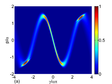
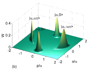
Figure 1: (Color online) (a) Plot of the probability distribution $P\left(p,\gamma\right)$ defined in Eq. (5 ) for $\alpha=7$ and $\gamma\in\left[-4\alpha\pi,4\alpha\pi\right]$. It shows that the states $\left|\alpha,\pm\gamma\right\rangle$ are also sufficiently distinguishable when $\gamma$ is around the values of $\alpha\pi(2l+1)$, $l=0$, $\pm 1$, $\pm 2$, $...$. (b) Plot of Wigner functions for states $\left|\pm\alpha,0\right\rangle$, and $\left|\alpha,\pm\gamma\right\rangle$ with $\alpha=7$ and $\gamma=\alpha\pi$ .

By taking $\alpha=7$, $\gamma\in\left[-4\alpha\pi,4\alpha\pi\right]$, we plot the probability distribution

$$P\left(p,\gamma\right)=\left|\psi_{\gamma}\left(p\right)\right|^{2}=e^{-\left|\alpha\right|^{2}}\left|\sum_{n}\frac{\alpha^{n}}{\sqrt{n!}}\mathrm{e}^{-\mathrm{i}\gamma\sqrt{n}}\phi_{n}\left(p\right)\right|^{2},$$ (5)

where $\phi_{n}\left(p\right)$ is the eigenfunction of the harmonic oscillator system in $p$ space.

We plot the probability distribution $W_{\alpha,\gamma}(x,p)$ for $\alpha$ $=\pm 7$, $\gamma=0$; $\alpha=7$, $\gamma=\pm\alpha\pi$. Fig. 1 shows that $\left|\alpha,\pm\gamma\right\rangle$ are also sufficiently distinguishable when $\gamma$ is around the values of $\alpha\pi(2l+1)$, with $l=0$, $\pm 1$, $\pm 2$, $...$. It is not true for the cases of $\left|l\right|\gg 1$, which is beyond our concern because they cannot be precisely prepared as $\left|l\right|$ increases in our scheme. It indicates that the state $c_{1}\left|\alpha,\gamma\right\rangle+c_{2}\left|\alpha,-\gamma\right\rangle$ can be considered as a Schrödinger cat state. Moreover, modified coherent state $\left|\alpha,\gamma\right\rangle$ is physically relevant. It can be prepared from the canonical coherent state $\left|\alpha,0\right\rangle$ by natural time evolution in a system with $\sqrt{n}$ spectrum. In the Ref. [32], it is shown that $\left|\alpha,\gamma\right\rangle$ can be obtained from $\left|\alpha,0\right\rangle$ by natural time evolution. However, we would like to point that the approximation in the Ref. [32]

$$\sum_{n=0}^{\infty}\alpha^{n}/\sqrt{n!}\mathrm{e}^{\mp\mathrm{i}\sqrt{n}\lambda t}$$ (6)

$$\approx \mathrm{e}^{\mp\mathrm{i}\alpha\lambda t/2}\sum_{n=0}^{\infty}\alpha^{n}/\sqrt{n!}\mathrm{e}^{\mp\mathrm{i}n\lambda t/2\alpha},$$

is not suitable for the purpose of quantum information processing, since the norm of the overlap between the exact and approximate wavefunctions is estimated as

$$\left|\mathrm{e}^{-\left|\alpha\right|^{2}}\sum_{n=0}^{\infty}\frac{\alpha^{2n}}{n!}\mathrm{e}^{-\mathrm{i}\pi\left(\alpha\sqrt{n}-n/2\right)}\right|$$ (7)

$$\approx \left|\frac{1}{\sqrt{2\pi}\alpha}\int_{-\infty}^{\infty}\exp\left[-\left(\frac{1}{2\alpha^{2}}-\frac{\mathrm{i}\pi}{8\alpha^{2}}\right)\left(x-\alpha^{2}\right)^{2}\right]\mathrm{d}x\right|$$

$$= 0.8868,$$

which is far from $1$. This is one of the reasons we are interested in the MCS. In the following section, we will demonstrate that the atom-field interaction can induce effective nonlinear spectrum of the photon. The cat state can be prepared by mapping the qubit state onto the field.

3 Effective separation of atom and field

In this section, we investigate the dynamics of the JC model and present the connection to the MCS. It has been pointed in the Ref. [32] that when the field is initially in a coherent state with large average photon number and the atom state is $\frac{1}{\sqrt{2}}\left(e^{-i\varphi}\left|e\right\rangle\pm\left|g\right\rangle\right)$, the time evolution of the atom-field system is

$$\frac{1}{\sqrt{2}}\left(\mathrm{e}^{-\mathrm{i}\varphi}\mathrm{e}^{\mp\mathrm{i}\frac{\lambda t}{2\alpha}}\left|g\right\rangle\pm\left|e\right\rangle\right)\mathrm{e}^{-\alpha^{2}/2}\sum_{n}\frac{\alpha^{n}}{\sqrt{n!}}\mathrm{e}^{-\mathrm{i}n\varphi}\mathrm{e}^{\mp\mathrm{i}\sqrt{n}\lambda t}\left|n\right\rangle.$$ (8)

It indicates that a MCS can be generated from a natural time evolution. To reveal the underlying mechanism of this process, we will reconsider this issue in an alternative way. The obtained result is applicable for a class of field states and will shed the light on the scheme of quantum information transfer from field to atom.

Consider a single-cavity JC model

$$H = \lambda\left(\sigma_{+}a+\sigma_{-}a^{{\dagger}}\right)+\frac{1}{2}\omega_{a}\sigma_{z}+\omega a^{\dagger}a,$$ (9)

$$\sigma_{+} = \left(\sigma_{-}\right)^{\dagger}=\left|e\right\rangle\left\langle g\right|,\sigma_{z}=\left|e\right\rangle\left\langle e\right|-\left|g\right\rangle\left\langle g\right|,$$ (10)

where $\omega$ is photon frequency, $\left|g\right\rangle$ and $\left|e\right\rangle$ denote the ground and excited states of atom with transition frequency $\omega_{a}$, and $\lambda$ is the atom-field coupling constant. Under the resonance condition $\omega_{a}=\omega$, it can be reduced to a simple form

$$H=\lambda\left(\sigma_{+}a+\sigma a^{\dagger}\right),$$ (11)

in the interaction picture. We notice that the Jaynes-Cummings model has been realized in the laboratory in several well-known ways [26, 27, 28, 29, 30] and employed to engineer states by using atom as a medium since almost two decades [31].

We note that the excitation number, $\mathcal{N}=\frac{1}{2}\sigma_{z}+a^{\dagger}a+\frac{1}{2}$ is a conservative quantity, i.e., $\left[\mathcal{N},H\right]=0$. So the Hamiltonian can be diagonalized in each $2\times 2$ invariant subspace. We start our analysis from Hamiltonian (11), which can be rewritten in the form

$$H=H_{\mathrm{1}}+H_{\mathrm{2}},$$ (12)

$$H_{\mathrm{1}} = \lambda(\mathrm{e}^{\mathrm{i}\varphi}\left|e\right\rangle\left\langle g\right|\sum_{n}\sqrt{n+1}\left|n\right\rangle\left\langle n\right|+\mathrm{e}^{-\mathrm{i}\varphi}\left|g\right\rangle\left\langle e\right|\sum_{n}\sqrt{n}\left|n\right\rangle\left\langle n\right|,)$$ (13)

$$H_{\mathrm{2}} = \lambda\sum_{n}\sqrt{n+1}\left(\mathrm{e}^{\mathrm{i}\varphi}\left|e\right\rangle\left\langle g\right|\left|n\right\rangle-\left|g\right\rangle\left\langle e\right|\left|n+1\right\rangle\right)\left(\mathrm{e}^{-\mathrm{i}\varphi}\left\langle n+1\right|-\left\langle n\right|\right),$$ (14)

by taking $\left\langle n+1\right|=$ $\mathrm{e}^{\mathrm{i}\varphi}\left(\left\langle n\right|+\mathrm{e}^{-\mathrm{i}\varphi}\left\langle n+1\right|-\left\langle n\right|\right)$, $\left\langle n\right|$ $=\mathrm{e}^{-\mathrm{i}\varphi}\left\langle n+1\right|$ $-\mathrm{e}^{-\mathrm{i}\varphi}\left\langle n+1\right|+\left\langle n\right|$, where $\varphi$ is an arbitrary real number.

For a separated state

$$\left|\phi\left(0\right)\right\rangle=\left(c_{1}\left|g\right\rangle+c_{2}\left|e\right\rangle\right)\sum_{n}f_{n}\left|n\right\rangle,$$ (15)

where $\left|c_{1}\right|^{2}+\left|c_{2}\right|^{2}=1$, and $\sum_{n}\left|f_{n}\right|^{2}=1$, one can reduce the Hamiltonian to the simple form under certain conditions. We note that if

$$f_{n}\approx\mathrm{e}^{\mathrm{i}\varphi}f_{n-1}\text{, }\left|f_{n}\right|^{2}\ll 1,$$ (16)

we have $\left|H_{\mathrm{2}}\left|\phi\left(0\right)\right\rangle\right|\ll\left|H_{\mathrm{1}}\left|\phi\left(0\right)\right\rangle\right|$, i.e., the dynamics of state $\left|\phi\left(0\right)\right\rangle$ is governed by the Hamiltonian $H_{\mathrm{1}}$ approximately. Now we focus on the Hamiltonian $H_{\mathrm{1}}$. In addition to the condition in Eq. (16), when we consider the field state satisfying

$$\bar{n}\gg\triangle n\gg 1,$$ (17)

where $\bar{n}$ denotes the average photon number with $\bar{n}$ $=\sum_{n_{1}}^{n_{2}}n\left|f_{n}\right|^{2}$, $\triangle n=n_{2}-n_{1}$, we can have $H_{\mathrm{1}}=H_{+}P_{+}+H_{-}P_{-}$. Here the projection operators $P_{\pm}$ for atom state are $P_{\pm}=\frac{1}{2}\left(\left|g\right\rangle\pm\mathrm{e}^{\mathrm{i}\varphi}\left|e\right\rangle\right)\left(\left\langle g\right|\pm\mathrm{e}^{-\mathrm{i}\varphi}\left\langle e\right|\right)$, which satisfy $P_{+}+P_{-}=1$ and $P_{+}P_{-}=0$. In the derivation, we have used the approximation $\left(n+1\right)^{1/2}\approx n^{1/2}+\frac{1}{2\bar{n}^{1/2}}$, under the condition in Eq. (17). The sub-Hamiltonians $H_{\pm}$ are in the form $H_{+}=-H_{-}=\frac{\lambda}{2\bar{n}^{1/2}}\left|e\right\rangle\left\langle e\right|+\lambda\sum_{n}\sqrt{n}\left|n\right\rangle\left\langle n\right|$.

Before further discussion of the implication of the obtained result, two distinguishing features need to be mentioned. First, the spectra of the photons in $H_{\pm}$ are $\pm\lambda\sqrt{n}$, which are related to the preparation of states $\left|\alpha,\pm\gamma\right\rangle$ from $\left|\alpha,0\right\rangle$ by natural time evolution, as mentioned above. This is crucial for the scheme to write the qubit state in the field. Second, we note that $H_{+}$ and $H_{-}$ have opposite sign, which leads to the time evolution of photons in two reverse directions respectively. This is crucial for the scheme to read the state from the field.

4 Quantum state transfer between atom and field

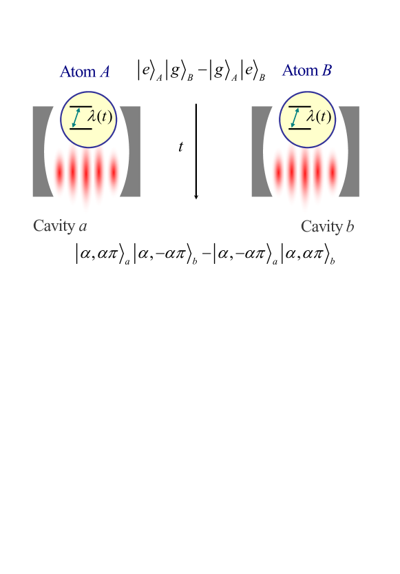
Figure 2: (Color online) Schematic illustration of the system for the entanglement transfer protocol. Atoms $A$ and $B$ are embedded in their respective cavities $a$ and $b$. Initially, two atoms are maximally entangled. The natural time evolution driven by the $A-a$ and $B-b$ interactions $\lambda\left(t\right)$ can transfer the $AB$ entanglement to the fields entanglement between cavities $a$ and $b$. The time dependence of coupling constant $\lambda\left(t\right)$ is explained in the text.

A state in the form of Eq. (15) can be rewritten as $\left|\phi\left(0\right)\right\rangle=\frac{1}{\sqrt{2}}\left[A\left(\left|g\right\rangle+\mathrm{e}^{\mathrm{i}\varphi}\left|e\right\rangle\right)+B\left(\left|g\right\rangle-\mathrm{e}^{\mathrm{i}\varphi}\left|e\right\rangle\right)\right]\times\sum_{n}\left|f_{n}\right|\mathrm{e}^{\mathrm{i}n\varphi}\left|n\right\rangle$, where $A=\frac{1}{\sqrt{2}}\left(c_{1}+\mathrm{e}^{-\mathrm{i}\varphi}c_{2}\right)$ and $B$ $=\frac{1}{\sqrt{2}}\left(c_{1}-\mathrm{e}^{-\mathrm{i}\varphi}c_{2}\right)$. Then we have

$$\left|\phi\left(t\right)\right\rangle= \frac{1}{\sqrt{2}}A\left(\left|g\right\rangle+\mathrm{e}^{-\mathrm{i}\frac{\lambda t}{2\bar{n}^{1/2}}}\mathrm{e}^{\mathrm{i}\varphi}\left|e\right\rangle\right)\sum_{n}\left|f_{n}\right|\mathrm{e}^{-\mathrm{i}\sqrt{n}\lambda t}\mathrm{e}^{\mathrm{i}n\varphi}\left|n\right\rangle$$ (18)

$$+\frac{1}{\sqrt{2}}B\left(\left|g\right\rangle-\mathrm{e}^{\mathrm{i}\frac{\lambda t}{2\bar{n}^{1/2}}}\mathrm{e}^{\mathrm{i}\varphi}\left|e\right\rangle\right)\sum_{n}\left|f_{n}\right|\mathrm{e}^{\mathrm{i}\sqrt{n}\lambda t}\mathrm{e}^{\mathrm{i}n\varphi}\left|n\right\rangle.$$

It is the superposition state of two independent evolution processes in which there are no interactions between atom and field. At the instants, $t_{l}=\left(2l+1\right)\tau$, $l=0,1,2,...$, $\tau=\bar{n}^{1/2}\pi/\lambda$, we have

$$\left|\phi\left(t_{l}\right)\right\rangle=\frac{\left|g\right\rangle-\left(-1\right)^{l}\mathrm{i}\mathrm{e}^{\mathrm{i}\varphi}\left|e\right\rangle}{\sqrt{2}}\left(A\left|\Phi_{+}^{l}\right\rangle+B\left|\Phi_{-}^{l}\right\rangle\right),$$ (19)

where $\left|\Phi_{\pm}^{l}\right\rangle=\sum_{n}\left|f_{n}\right|\mathrm{e}^{\mp\mathrm{i}\sqrt{n}\lambda t_{l}}\mathrm{e}^{\mathrm{i}n\varphi}\left|n\right\rangle$. As one can see in the formula above, an arbitrary atom state can retrieve a pure state at the instants $t_{l}$. Remarkably, the initial atomic state $\left(A,B\right)$ is mapped on the field state if $\left|\Phi_{+}^{l}\right\rangle$ and $\left|\Phi_{-}^{l}\right\rangle$ are orthogonal, while the atom is always in the state $\left(\left|g\right\rangle-\mathrm{i}\mathrm{e}^{\mathrm{i}\varphi}\left|e\right\rangle\right)/\sqrt{2}$. This is termed as “attractor” in Ref. [32], which considered the initial field state being a coherent state. However, according to our analysis, the initial state can be a class of field states. To demonstrate this point, we consider the simplest field state, a top-hat state as the form

$$f_{n}=\left\{\begin{array}[]{c}1/\Delta\text{, }\bar{n}-\Delta/2\leqslant n<\bar{n}+\Delta/2\\ 0,\text{elsewhere}\end{array}\right..$$ (20)

Submitting $f_{n}$ to Eq. (18) and taking $\varphi=0$, $t=\tau=\bar{n}^{1/2}\pi/\lambda$, yields

$$\left|\phi\left(\tau\right)\right\rangle= \frac{1}{\sqrt{2}}A\left(\left|g\right\rangle-\mathrm{i}\left|e\right\rangle\right)\frac{1}{\Delta}\sum_{n-\Delta/2}^{n+\Delta/2-1}\mathrm{e}^{-\mathrm{i}\sqrt{n}\bar{n}^{1/2}\pi}\left|n\right\rangle$$ (21)

$$+\frac{1}{\sqrt{2}}B\left(\left|g\right\rangle-\mathrm{i}\left|e\right\rangle\right)\frac{1}{\Delta}\sum_{n-\Delta/2}^{n+\Delta/2-1}\mathrm{e}^{\mathrm{i}\sqrt{n}\bar{n}^{1/2}\pi}\left|n\right\rangle.$$

To verify this approximate result, we compute the norm of the overlap $\digamma\left(t\right)$ between the analytical and numerical final states. For the cases of $\Delta=5$, $10$, and $20$, $\bar{n}=49$, we have $\digamma\left(\tau\right)=$ $0.9001$, $0.9955$, and $0.9738$. It indicates that for a given $\bar{n}$, an optimal $\Delta$ can lead to a perfect fidelity. Thus the coherent state $\left|\alpha\right\rangle$ is not the unique field state leading to the separation of the atom and field.

Nevertheless, we still take the coherent state $\left|\alpha\right\rangle$ as an example to illustrate our scheme in this paper. From Eq. (19), we note that the initial state $\left(A,B\right)$ can never go back to the atom as expected. This procedure can be employed to transfer or store the quantum information to the field. However, the stored information can not be read out from the field via the further time evolution alone this path, as expected in a general scheme, the initial state is revival periodically.

Qubit decoherence times are on the order of a few microseconds, in particular, that for the transmon is about $\sim$4 $\mu$s. As a result, the implementation, including the preparation of the cat state and adiabatic adjustment of the parameters, should be accomplished within the time much shorter than the decoherence time. According to recent experiments, the decoherence time can be a few dozen times longer than the $\tau$[33, 34].

Considering the initial field state as a coherent state $\left|\alpha,0\right\rangle$, with $f_{n}=\mathrm{e}^{-\left|\alpha\right|^{2}/2}\alpha^{n}/\sqrt{n!}$ and $\varphi=0$, we have

$$\left|\phi\left(\tau\right)\right\rangle=\frac{1}{\sqrt{2}}\left(\left|g\right\rangle-\mathrm{i}\left|e\right\rangle\right)\left(A\left|\alpha,\alpha\pi\right\rangle+B\left|\alpha,-\alpha\pi\right\rangle\right)\text{.}$$ (22)

Then the quantum information in the atom is encoded into the field. We would like to point that, the initial state of the atom cannot be revival again as expected, not like the swap gate.

Another interesting feature in such dynamic process is that two effective Hamiltonians for atoms differ only in an opposite sign, i.e., $H_{+}=-H_{-}$. It shows that two atom states $\left(\left|g\right\rangle+\mathrm{e}^{\mathrm{i}\varphi}\left|e\right\rangle\right)/\sqrt{2}$ and $\left(\left|g\right\rangle-\mathrm{e}^{\mathrm{i}\varphi}\left|e\right\rangle\right)/\sqrt{2}$ evolve in the same way but in opposite time directions. It is crucial for the scheme of reading out the information from the field.

A trivial way to retrieve the initial atomic state is to switch the sign of interaction strength $\lambda$ to realize the reversed time evolution. Alternative operation can also implement the same task: flipping the states $\left(\left|g\right\rangle-\mathrm{i}\mathrm{e}^{\mathrm{i}\varphi}\left|e\right\rangle\right)/\sqrt{2}\rightarrow\left(\left|g\right\rangle+\mathrm{i}\mathrm{e}^{\mathrm{i}\varphi}\left|e\right\rangle\right)/\sqrt{2}$ by the external pulse. (rotation operator $\mathrm{e}^{\mathrm{i}\pi\left(\sigma_{z}+1\right)/2}=-\sigma_{z}$) Then taking the state $\left|\widetilde{\phi}\left(0\right)\right\rangle=\left(\left|g\right\rangle+\mathrm{i}\left|e\right\rangle\right)\left(A\left|\alpha,\alpha\pi\right\rangle+B\left|\alpha,-\alpha\pi\right\rangle\right)/\sqrt{2}$, as the initial state, we have $\left|\widetilde{\phi}\left(\tau\right)\right\rangle=-\sigma_{z}\left|\phi\left(0\right)\right\rangle$.

Although this conclusion is achieved in the framework of approximation, we would like to point that such a time-reversal process is exact. The underlying mechanism is similar to the phenomenon of spin echo. We note that the Hamiltonian (11) obeys the anti-commutation relation

$$\left\{\sigma_{z},H\right\}=0.$$ (23)

Then for an arbitrary initial state $\psi\left(0\right)$ and an arbitrary time interval $t$, we have $\psi^{\prime}\left(2t\right)$ $\equiv\left(-\sigma_{z}\right)\mathrm{e}^{-\mathrm{i}Ht}\left(-\sigma_{z}\right)\mathrm{e}^{-\mathrm{i}Ht}\psi\left(0\right)$ $=\mathrm{e}^{\mathrm{i}Ht}\mathrm{e}^{-\mathrm{i}Ht}\psi\left(0\right)=\psi\left(0\right)$.

It represents a process similar to the spin echo, refocusing the information spreading to the field. The atom retrieves its initial state under the operation of spin flip at half time. We note that the relation in Eq. (23) requires the resonance condition in an atom-field system. Then resonance is crucial for the reversal process. This feature can be applied to the atom-field system without rotating-wave-approximation. On the other hand, the original Hamiltonian $H_{\text{{S}}}=H+\omega\left(\mathcal{N-}\frac{1}{2}\right)$ in the Schrodinger picture has $\left\{\sigma_{z},H_{\text{{S}}}\right\}\neq 0$. However, we still have $\psi_{\mathrm{s}}^{\prime}\left(2t\right)\equiv\left(-\sigma_{z}\right)e^{-\mathrm{i}H_{\mathrm{S}}t}\left(-\sigma_{z}\right)e^{-\mathrm{i}H_{\mathrm{S}}t}\psi\left(0\right)$ $=\left(-\sigma_{z}\right)e^{-\mathrm{i}Ht}e^{-\mathrm{i}\omega\left(\mathcal{N-}\frac{1}{2}\right)t}\left(-\sigma_{z}\right)e^{-\mathrm{i}Ht}e^{-\mathrm{i}\omega\left(\mathcal{N-}\frac{1}{2}\right)t}\psi\left(0\right)$ $=e^{-2\mathrm{i}\omega\left(\mathcal{N-}\frac{1}{2}\right)t}e^{\mathrm{i}Ht}e^{-\mathrm{i}Ht}\psi\left(0\right)$ $=e^{-2\mathrm{i}\omega\left(\mathcal{N-}\frac{1}{2}\right)t}\psi\left(0\right)$, due to the relation $\left[\sigma_{z},\mathcal{N}\right]=0$. We note that operator $e^{-2\mathrm{i}\omega\left(\mathcal{N-}\frac{1}{2}\right)t}$ cannot induce any unexpected effects for the initial state $\psi\left(0\right)$ we consider in this paper.

We would like to point that the separation of atom and field is approximate. In fact, the atom and field always interact with each other. The effective separation is the result of interference. We note that the approximation condition require that the phase between $\left|n\right\rangle$ and $\left|n+1\right\rangle$ is arbitrary but identical, i.e., $\varphi$ is $n$-dependent. However, the evolved state will acquire an extra phase being proportional to $\sqrt{n}t$ rather than $nt$. Then, as time increases, the deviation of the evolved wave function from the approximation condition get large. In order to estimate the time scale within which the effective Hamiltonian is available, we plot of the Loschmidt echo

$$L\left(t\right)=\left|\left\langle\psi\left(0\right)\right|\mathrm{e}^{\mathrm{i}Ht}\mathrm{e}^{-\mathrm{i}H_{\mathrm{1}}t}\left|\psi\left(0\right)\right\rangle\right|,$$ (24)

which is a estimate of the differentiating effects for $H$ and $H_{\mathrm{1}}$. From Fig. 3, we see that $L\left(t\right)$ depends on the $\alpha$ in the initial state. For $\alpha=10$, $L\left(t\right)$ can be more than $0.95$ at $t=\tau$, and $0.9$ within $t=8\tau$. Then we see that the effective Hamiltonian is available in a short time.

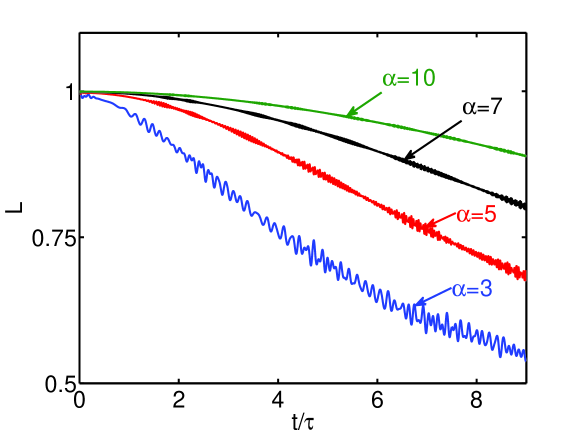
Figure 3: (Color online) Plots of the Loschmidt echo $L\left(t\right)$ defined in Eq. (24 ) for the cases of $\alpha=3$, $5$, $7$ and $10$. It indicates that the decay of $L\left(t\right)$ becomes slow as the average photon number increase.

In order to quantitatively evaluate the extent of approximation of the effective Hamiltonian and demonstrate the write and read scheme, the numerical method is employed to simulate the dynamic processes of quantum state transfer.

For the writing process, we take the initial state as $\left|\phi\left(0\right)\right\rangle=\frac{1}{\sqrt{2}}\left(\left|g\right\rangle+\left|e\right\rangle\right)\left|\alpha,0\right\rangle$. The fidelity of the state transfer is $F_{W}\left(t\right)=\left|\left\langle\phi\left(0\right)\right|\mathrm{e}^{\mathrm{i}Ht}\left|\phi_{W}\right\rangle\right|$, where $\left|\phi_{W}\right\rangle=\left(\left|g\right\rangle-\mathrm{i}\left|e\right\rangle\right)/2\left|\alpha,\alpha\pi\right\rangle$ is the target state. Similarly, the fidelity for the reading process is defined as $F_{R}\left(t\right)=\left|\left\langle\psi\left(0\right)\right|\mathrm{e}^{\mathrm{i}Ht}\left|\psi_{R}\right\rangle\right|,$ where the initial state $\left|\psi\left(0\right)\right\rangle=-\sigma_{z}\left|\phi_{W}\right\rangle$ and the target state is $\left|\psi_{R}\right\rangle$ $=-\sigma_{z}\left|\phi\left(0\right)\right\rangle=\frac{1}{\sqrt{2}}\left(\left|g\right\rangle-\left|e\right\rangle\right)\left|\alpha,0\right\rangle$. Straightforward derivation shows that $F_{W}\left(t\right)=F_{R}\left(t\right)\equiv F\left(t\right)$. In Fig. 4, $F\left(t\right)$ is plotted for the cases of $\alpha=3,5,7,$ and $10$, which shows that the fidelity increases with $\alpha$ and the QST approaches to perfect when the average photon number is more than two dozen.

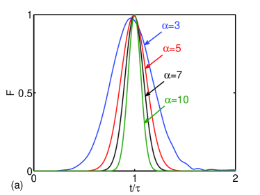
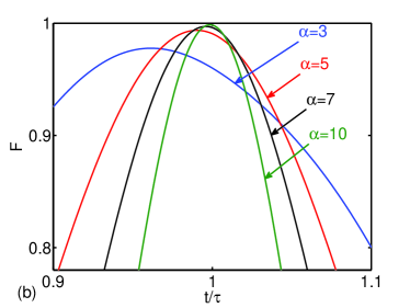
Figure 4: (Color online) Plots of the fidelity $F\left(t\right)$ as function of time for the cases of $\alpha=3$, $5$, $7$ and $10$. (b) is a zoom-in figure of (a). The fidelity $F\left(t\right)$ in each cases has a maximum at the instant $t_{m}$. Both $F\left(t_{m}\right)$ and $t_{m}/\tau$ tend to $1$ as $\alpha$ increases.

5 Entanglement transfer

A straightforward application of the above analysis is generation of a non-local Schrödinger cat state, which is a fundamental resource in fault-tolerant quantum computing and quantum communication. In this section, we study the dynamics of entanglement transfer in a system composed of two initially entangled atoms, each located in one of two non-interacting cavities. A schematic illustration of the system is given in Fig. 2. The Hamiltonian of the set-up is [6]

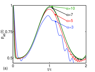
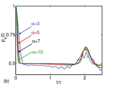
Figure 5: (Color online) Plot of the purities $p_{ab}\left(t\right)$ and $p_{a}\left(t\right)$ for the type of initial state in Eq. (26) as a function of time (in unit of $\tau=\alpha\pi/\lambda$) and parameter $\alpha$. It shows that the maximal entanglement between two distant cavities can be generated for large $\alpha$.

$$H_{AB}=\lambda(a^{\dagger}\sigma_{-}^{A}+b^{\dagger}\sigma_{-}^{B}+\mathrm{H.c.}),$$ (25)

where $\sigma_{-}^{A}(\sigma_{-}^{B})$ and $a^{\dagger}(b^{\dagger})$ are the corresponding operators of the atom and field in the cavity $A(B)$, respectively, and $\lambda$ is the coupling constant between the atoms and their cavities. Here we only consider the case of resonance.

The separation of systems $A$ and $B$ makes the dynamics of whole system easier to be understood [35]. It is predictable that the entanglement of two atoms can be perfectly transferred to the fields $a^{\dagger}$ and $b^{\dagger}$, which leads to generate a non-local Schrödinger cat state in large $\alpha$ limit.

For finite $\alpha$, to demonstrate the process of entanglement transfer, we compute the purity $p_{ab}$ of the field states in two cavities, as well as that $p_{a}$ (or $p_{b}$) for a single cavity. The former is the measure of the entanglement between the atoms and the fields, while the later is that between fields in two cavities. Here the purities for an arbitrary state $\left|\phi\right\rangle$ are defined as $p_{ab}=\mathrm{Tr}\left(\rho_{ab}\right)^{2}$, $p_{a}=\mathrm{Tr}\left(\rho_{a}\right)^{2},$ with $\rho_{ab}=\mathrm{Tr}_{\mathrm{AB}}\left(\left|\phi\right\rangle\left\langle\phi\right|\right)$, $\rho_{a}=\mathrm{Tr}_{\mathrm{b}}\left(\rho_{ab}\right)$, where Tr${}_{\mathrm{AB}}(.)$ and Tr${}_{\mathrm{b}}(.)$ denote the operation of tracing out all atomic states and field $b$ states, respectively.

Now we examine the efficiency of the entanglement transfer from the atoms to the field for finite $\alpha$. The initial state is

$$\left|\phi\left(0\right)\right\rangle=\frac{\left|e\right\rangle_{A}\left|g\right\rangle_{B}-\left|g\right\rangle_{A}\left|e\right\rangle_{B}}{\sqrt{2}}\left|\alpha,0\right\rangle_{a}\left|\alpha,0\right\rangle_{b},$$ (26)

which denotes a maximally entangled $AB$ state, but an unentangled $ab$ state. According to our analysis above mentioned, for sufficient large $\alpha$, the state evolves to

$$\left|\phi\left(\tau\right)\right\rangle = \frac{1}{2\sqrt{2}}\left(\left|g\right\rangle_{A}-\mathrm{i}\left|e\right\rangle_{A}\right)\left(\left|g\right\rangle_{B}-\mathrm{i}\left|e\right\rangle_{B}\right)$$ (27)

$$\left(\left|\alpha,\alpha\pi\right\rangle_{a}\left|\alpha,-\alpha\pi\right\rangle_{b}-\left|\alpha,-\alpha\pi\right\rangle_{a}\left|\alpha,\alpha\pi\right\rangle_{b}\right),$$

at the instant $\tau$. We can see that the atoms $AB$ state is unentangled. Furthermore, fields $a$ and $b$ are maximally entangled if each cavity is regarded as a qubit. Quantities $p_{ab}$ and $p_{a}$ (or $p_{b}$) of the state $\left|\phi\left(\tau\right)\right\rangle$ reflect this feature: Purity $p_{ab}=1$ indicates that the field state is in pure state, being separable from the state of atoms. Purity $p_{a}=0.5$ indicates the maximal entanglement fields $a$ and $b$ as a two-qubit system. In this sense, the later is only an essential condition for the existence of state $\left|\phi\left(\tau\right)\right\rangle$. Nevertheless, we believe that the simultaneous occurrence of $p_{ab}=1$ and $p_{a}=0.5$ can be regarded as the evidence of the existence of the state $\left|\phi\left(\tau\right)\right\rangle$ in the context of the present model.

The purities $p_{ab}\left(t\right)$ and $p_{a}\left(t\right)$ for the state evolving from the initial state given by Eq. (26) are plotted in Fig. 5 for the cases of $\alpha=3$, $5$, $7$ and $10$. As seen from the plots, purities $p_{ab}\left(t\right)$ and $p_{a}\left(t\right)$ approach to $1$ and $0.5$, respectively, at time $\tau$ as $\alpha$ increases. In order to estimate the time scales associated with the initial decay, we employ the curve fitting for the numerical results in Fig. 5 and obtained the fitted function as $p_{a}\left(t\right)\approx p_{b}\left(t\right)$ $\approx 0.5\exp\left(-\lambda^{2}t^{2}\right)+0.5$ $=0.5\exp\left[-\alpha^{2}\pi^{2}\left(t/\tau\right)^{2}\right]+0.5$. By the same procedure, the fitted function around the revival can be obtained as $p_{ab}\left(t\right)$ $\approx 0.5\sin^{4}\left(\lambda t/2\alpha\right)\exp\left(-\lambda^{2}t^{2}/8\alpha^{4}\right)+0.5$ $=0.5\sin^{4}\left[\pi\left(t/\tau\right)/2\right]\exp\left[-\pi^{2}\left(t/\tau\right)^{2}/8\alpha^{2}\right]+0.5$, which indicates the width of the revival as $w\approx 0.73\tau$ $=0.73\alpha\pi/\lambda$. It shows that the entanglement can be perfectly transferred from atoms to fields. It also provides an alternative scheme for preparation of non-local superpositions of quasi-classical light states.

Before ending this paper, we want to stress that there is an important feature of the scenario. Actually, the dynamic processes in above schemes are invariant if the coupling strength $\lambda$ is time dependent. All the derivation above is still true if we replace $\lambda\Delta t$ by $\int_{0}^{\Delta t}\lambda\left(t\right)dt$. One can take the interaction in the form $\lambda\left(t\right)=\lambda_{0}\mathrm{exp}\left(-\alpha^{2}t^{2}\right)$ which can be used to turn an initial coherent field into a Schrödinger cat state. It ensures the switching control feasible for schemes in experiment. In addition, the swiching processes of $\lambda$ in two cavities cannot be simultaneous. This alllows the generation of entanglement between a cavity and a distant atom.

Nevertheless, there is always dissipation in cavities. The effect of dissipation on a macroscopic superposition of quantum states has been studied with the use of a Markovian master-equation approach. An approximate solution was given for the JC model with cavity losses by J.Gea-Banacloche in 1993 [36]. It has been reported that, although the dissipation destroys the coherence of the macroscopic superposition very rapidly, preparation and observation of the cat state should be possible, which depends on a factor $F\left(t\right)$ characterizing the cavity quality, or describing the effect of dissipation. According to their analysis, when the magnitude of $F\left(t\right)$ is close to $1$, the effect of dissipation is slight. More explicitly, at the revival time $t_{R}=2\tau$, the corresonding factor yields

$$\left|F\left(t_{R}\right)\right|\approx e^{-4\pi\kappa\bar{n}^{3/2}/\lambda},$$ (28)

where $\kappa$ is the damping rate of photon to the reservoir at zero temperature. In our paper, because there is no interaction between two cavities, the effect of dissipation should be the same as the result in ref. [36]. So the outcome should be observable in the system with $\kappa/\lambda\sim 10^{-5}$, which predicts $\left|F\left(t_{R}\right)\right|\approx 0.9844$, when $\bar{n}=25$.

However, according to the current experiment, the realization of our scheme is difficult due to the dissipation. It is reported that parameters $\lambda=2\pi\times 75\mathrm{MHz}$ and $\kappa=2\pi\times 3.5\mathrm{MHz}$ can be achievable in optical cavities with the wave-length in the region $630-850$nm in recent experiments [37, 38], which result in $\left|F\left(t_{R}\right)\right|\approx 0$. In another case, the optical fiber decay at a $852$nm wavelength is about $2.2$dB/km [39, 40], which corresponds to the fiber decay rate of $\kappa=0.152\mathrm{MHz}$. In this case, the $\left|F\left(t_{R}\right)\right|\approx 0.6025$, which is still lower.

6 Summary

In summary, we have presented a scheme for state transfer between atom and cavity field in Jaynes-Cummings model. It is shown that the nonlinearity arising from the atom-field coupling can induce the generation of modified coherent states, which can be shown to be macroscopically distinguishable as standard coherent states. We have shown that an arbitrary atom state can be mapped onto the field as Schrödinger cat state via natural time evolution. The reversal process can also be achieved in the aid of spin-echo-like technique. We also found that the coherent state is just one of a class of field states, which can be used as an initial state to perform this task. This result can be extended to non-interacting multi-cavity system. Analytical and numerical calculations have demonstrated that the dynamic process on two-cavity system can provide an alternative scheme for preparation of non-local superpositions of quasi-classical light states. Moreover, we discussed the effect of dissipation.

References

• [1] J. A. Wheeler and W. H. Zurek, Quantum Theory and Measurement (Princeton: Princeton University Press, 1983).
• [2] C. C. Gerry and P. L. Knight, Introductory Quantum Optics (Cambridge: Cambridge University Press, 2005).
• [3] S. Takagi, Macroscopic Quantum Tunneling (Cambridge: Cambridge University Press, 2002).
• [4] M. A. Nielsen and I. L. Chuang, Quantum Computation and Quantum Information (Cambridge: Cambridge University Press, 2001).
• [5] C. E. A. Jarvis, D. A. Rodrigues, B. L. Györffy, T. P. Spiller, A. J. Short and J. F. Annett, New J. Phys. 11 (2009) 103047.
• [6] J.-P. Gazeau, Coherent States in Quantum Physics (Berlin: Wiley-VCH Press, 2009).
• [7] P. T. Cochrane, G. J. Milburn and W. J. Munro, Phys. Rev. A 59 (1999) 2631.
• [8] H. Jeong and M. S. Kim, Phys. Rev. A 65 (2002) 042305.
• [9] T. C. Ralph, A. Gilchrist, G. J. Milburn, W. J. Munro and S. Glancy, Phys. Rev. A 68 (2003) 042319.
• [10] A. P. Lund, T. C. Ralph and H. L. Haselgrove, Phys. Rev. Lett. 100 (2008) 030503.
• [11] A. Ourjoumtsev, H. Jeong, R. Tualle-Brouri and P. Grangier, Nature 448 (2007) 784.
• [12] J. S. Neergaard-Nielsen, B. M. Nielsen, C. Hettich, K. Mølmer and E. S. Polzik, Phys. Rev. Lett. 97 (2006) 083604.
• [13] H. Takahashi, K. Wakui, S. Suzuki, M. Takeoka, K. Hayasaka, A. Furusawa and M. Sasaki, Phys. Rev. Lett. 101 (2008) 233605.
• [14] T. Gerrits, S. Glancy, T. S. Clement, B. Calkins, A. E. Lita, A. J. Miller, A. L. Migdall, S. W. Nam, R. P. Mirin and E. Knill,arXiv:1004.2727 (2011).
• [15] L. G. Lutterbach and L. Davidovich, Phys. Rev. Lett. 78 (1996) 13.
• [16] K. Vogel and H. Risken, Phys. Rev. A 40 (1989) 2847.
• [17] D. T. Smithey et al., Phys. Rev. Lett. 70 (1993) 1244.
• [18] U. Leonhardt and H. Paul, Phys. Rev. Lett. 72 (1994) 4086.
• [19] G. M. D’Ariano et al., Phys. Rev. A 52 (1995) R1801.
• [20] T. J. Dunn et al., Phys. Rev. Lett. 74 (1995) 884.
• [21] S. Wallentowitz and W. Vogel, Phys. Rev. Lett. 75 (1995) 2932.
• [22] C. D’Helon and G. Milburn, Phys. Rev. A 54 (1996) R25.
• [23] J. F. Poyatos et al., Phys. Rev. A 53(1996) R1966.
• [24] K. Banaszek and K. Wókiewicz, Phys. Rev. Lett. 76 (1996) 4344.
• [25] S. Wallentowitz and W. Vogel, Phys. Rev. A 53 (1996) 4528.
• [26] M. Brune, F. Schmidt-Kaler, A. Maali, J. Dreyer, E. Hagley, J. M. Raimond and S. Haroche, Phys. Rev. Lett. 76 (1996) 1800.
• [27] D. M. Meekhof, C. Monroe, B. E. King, W. M. Itano and D. J. Wineland, Phys. Rev. Lett. 76 (1996) 1796.
• [28] A. Boca, R. Miller, K. M. Birnbaum, A. D. Boozer, J. McKeever and H. J. Kimble, Phys. Rev. Lett. 93 (2004) 233603.
• [29] J. Li, M. P. Silveri, K. S. Kumar, J.-M. Pirkkalainen, A. Vepsäläinen, W. C. Chien, J. Tuorila, M. A. Sillanpää, P. J. Hakonen, E. V. Thuneberg and G. S. Paraoanu, Nature Communications 4 (2013) 1420.
• [30] J.-M. Pirkkalainen, S. U. Cho, J. Li, G. S. Paraoanu, P. J. Hakonen and M. A. Sillanpää, Nature 494 (2013) 211.
• [31] C. K. Law, J. H. Eberly, Phys. Rev. Lett. 76 (1996) 1055.
• [32] J. Gea-Banacloche, Phys. Rev. A 44 (1991) 5913.
• [33] Ö. E. Müstecaplıoğlu, Phys. Rev. A 83 (2011) 023805.
• [34] T. Liu, M. Feng, W. L. Yang, J. H. Zou, L. Li, Y. X. Fan and K. L. Wang, Phys. Rev. A 88 (2013) 013820.
• [35] M. Yönac, T. Yu and J. H. Eberly, J. Phys. B 40 (2007) S45.
• [36] J. Gea-Banacloche, Phys. Rev. A 47 (1993) 3.
• [37] S. M. Spillane, T. J. Kippenberg, K. J. Vahala, E. Wilcut and H. J. Kimble, Phys. Rev. A 71 (2005) 013817.
• [38] J. R. Buck and H. J. Kimble, Phys. Rev. A 67 (2003) 033806.
• [39] K. J. Gordon, V. Fernandez, P. D. Townsend and G. S. Buller, IEEE J. Quantum Electron. 40 (2004) 900–908.
• [40] S. B. Zheng, C. P. Yang and F. Nori, Phys. Rev. A 82 (2010) 042327.