Damping of the quadrupole mode in a two-dimensional Fermi gas

Abstract

In a recent experiment [E. Vogt et al., Phys. Rev. Lett. 108, 070404 (2012)], quadrupole and breathing modes of a two-dimensional Fermi gas were studied. We model these collective modes by solving the Boltzmann equation via the method of phase-space moments up to fourth order, including in-medium effects on the scattering cross section. In our analysis, we use a realistic Gaussian potential deformed by the presence of gravity and magnetic field gradients. We conclude that the origin of the experimentally observed damping of the quadrupole mode, especially in the weakly interacting (or even non-interacting) case, cannot be explained by these mechanisms.

I Introduction

Two-dimensional (2D) Fermi systems are particularly interesting, since both quantum and interaction effects are in this case stronger than in three dimensions (3D). The first experimental realization of a 2D Fermi gas with trapped atoms was reported in 2010 Martiyanov . The configuration obtained in this experiment and in the subsequent ones is an array of pancake-shaped clouds, obtained by slicing a 3D cloud with a one-dimensional periodic potential. These gases can be considered as 2D ones if the motion of particles in the axial direction is frozen to the lowest energy level.

In a recent experiment, the collective breathing and quadrupole modes of a gas of ⁴⁰K atoms trapped in this geometry were studied Vogt2012 . The interaction strength between the two hyperfine states and the temperature were varied in order to identify the transition from the collisionless to the hydrodynamic regime in the case of the quadrupole mode, and to confirm, in the case of the breathing mode, the dynamical scaling predicted a few years ago Pitaevskii . In a hydrodynamic picture, the damping of the quadrupole mode is related to the shear viscosity of the 2D gas: in particular, from the experimental results one can extract the temperature dependence of the shear viscosity.

A number of theoretical studies dealing with this experiment have already appeared Bruun2012 ; Schafer2012 ; Enss2012 ; WuZhang2012_2d ; Baur2013 . In Refs. Bruun2012 ; Schafer2012 the shear viscosity and spin-diffusion coefficients were computed from kinetic theory in the hydrodynamic regime. Surprisingly, it was found that the quantitative agreement with data was better in the collisionless regime. In LABEL:Enss2012, in-medium modifications of the scattering cross-section were included in the calculation of the shear viscosity, leading to a maximum damping rate as high as the experimental one under the assumption that the hydrodynamic approach was valid. In LABEL:WuZhang2012_2d, the Boltzmann equation was numerically solved in the local relaxation-time approximation (the relaxation time being calculated with the free-space cross section). The authors found a reasonable agreement with the experimental data in the case of moderate quantum degeneracy and not too strong interactions, if the computed damping was shifted upwards by a small constant value, introduced to account for additional effects like trap anharmonicity that had to be there since the experiment observed a finite damping of the dipole mode. In the most recent work by Baur et al. Baur2013 , the in-medium scattering cross-section was included into the Boltzmann equation (as it was done before in 3D Riedl2008 ; Chiacchiera2009 ) which was then solved in an approximate way by using the method of second-order phase-space moments. They conclude that they can well describe the experimental results, apart from an offset in the damping rate (see caption of Fig. 2 of LABEL:Baur2013).

In the case of collective modes in 3D Fermi gases, it was found that in order to quantitatively reproduce the result of a numerical solution of the Boltzmann equation Lepers2010 , the method of second-order moments was insufficient and higher-order moments had to be included. The inclusion of fourth-order moments improved a lot the agreement between theory and experiment in the case of the quadrupole mode Chiacchiera2011 . Furthermore, by using moments up to third order, it was possible to describe the effects of the trap anharmonicity (frequency shift and damping) on the sloshing mode Pantel2012 in 3D. Higher-order moments were also used in the context of 2D systems to describe collective modes in dipolar Fermi gases Babadi2012 .

In the present work, we will extend the analysis of the paper by Baur et al. Baur2013 . We will include all phase-space moments up to fourth order and study the effect of a realistic form of the trap potential having a gaussian shape with additional linear terms due to gravity and magnetic-field gradients. All this causes some damping of the quadrupole mode even in the non-interaction regime, but not as strong as the one observed in the experiment. We will also discuss other possible sources of damping like dephasing between different slices and the time-of-flight (TOF) before the measurement of the quadrupole moment, but they are all too weak to explain the data.

Our paper is organized as follows. In Sec. II, we briefly summarize the formalism. In Sec. III we investigate the convergence of the moments method to existing numerical solutions of the Boltzmann equation. In Sec. IV, we try to model as closely as possible the experiment Vogt2012 , and in Sec. V we draw our conclusions.

Throughout the paper, we use units with $\hbar=k_{B}=1$ ($\hbar=h/2\pi$ and $k_{B}$ being the reduced Planck constant and the Boltzmann constant, respectively). In a harmonic trap with average frequency $\bar{\omega}_{r}$, it is convenient to work with so-called “trap units”, e.g., the energy unit $\hbar\bar{\omega}_{r}$, the length unit $l_{\mathit{ho}}=\sqrt{\hbar/m\bar{\omega}_{r}}$, etc, $m$ being the atom mass. Furthermore, the Fermi energy $E_{F}=k_{B}T_{F}$ and Fermi momentum $k_{F}$ of a 2D trapped gas are defined by $E_{F}=\hbar\bar{\omega}_{r}\sqrt{N}$ and $k_{F}=\sqrt{2mE_{F}}/\hbar$.

II Formalism

II.1 Boltzmann equation in 2D

We consider a two-component ($\uparrow,\downarrow$) Fermi gas of $N$ atoms of mass $m$ that can move only in two dimensions ($x,y$). For a balanced mixture and “spin”-independent modes, it is enough to consider a single phase-space distribution function $f=f_{\uparrow}=f_{\downarrow}$, normalized to $\int d^{2}rd^{2}p/(2\pi)^{2}f(\bm{\mathrm{r}},\bm{\mathrm{p}})=N/2$, where $\bm{\mathrm{r}}=(x,y)$, $\bm{\mathrm{p}}=(p_{x},p_{y})$. Averages are computed as

$$\langle q\rangle(t)=\frac{2}{N}\int\frac{d^{2}rd^{2}p}{(2\pi)^{2}}f(\bm{\mathrm{r}},\bm{\mathrm{p}},t)q(\bm{\mathrm{r}},\bm{\mathrm{p}})\,.$$ (1)

At equilibrium, the distribution is given by the Fermi function

$$f_{\mathit{eq}}(\bm{\mathrm{r}},\bm{\mathrm{p}})=\frac{1}{e^{\beta\left(\frac{\bm{\mathrm{p}}^{2}}{2m}+V_{T}(\bm{\mathrm{r}})-\mu_{0}\right)}+1},$$ (2)

where $\beta=1/T$, $V_{T}$, and $\mu_{0}$ are the inverse temperature, the trap potential, and the chemical potential, respectively. Note that we neglect a possible mean-field potential, since in Refs. Chiacchiera2009 and Pantel2012 we have shown (in the 3D case) that it does not substantially affect the properties of the collective modes.

For small deviations from equilibrium, the change of the phase-space distribution $\delta f=f-f_{\mathit{eq}}$ can be written as Landau10

$$\delta f(\bm{\mathrm{r}},\bm{\mathrm{p}},t)=f_{\mathit{eq}}\bar{f}_{\mathit{eq}}\Phi(\bm{\mathrm{r}},\bm{\mathrm{p}},t)\,,$$ (3)

where $\bar{f}=1-f$. The prefactor $f_{\mathit{eq}}(1-f_{\mathit{eq}})$ takes care of the rapid variation of $\delta f$ around the Fermi surface, so that $\Phi$ can be considered a smooth function of $\bm{\mathrm{r}}$ and $\bm{\mathrm{p}}$. Then the linearized Boltzmann equation becomes

$$f_{\mathit{eq}}\bar{f}_{\mathit{eq}}\Big{(}\dot{\Phi}+\Big{\{}\Phi,\frac{p^{2}}{2m}+V_{T}(\bm{\mathrm{r}})\Big{\}}+\beta\frac{\bm{\mathrm{p}}}{m}\cdot\bm{\nabla}_{r}\delta V\Big{)}=-I[\Phi]\,,$$ (4)

where $\{\cdot,\cdot\}$ denotes the Poisson bracket and $\delta V$ is a perturbation of the trap potential used to excite the collective mode. Usually we consider a perturbation of the form of a $\delta$ pulse,

$$\delta V(\bm{\mathrm{r}},t)=\delta(t)\hat{V}(\bm{\mathrm{r}})\,.$$ (5)

The linearized collision integral $I[\Phi]$ reads

$$I[\Phi]=\int\frac{d^{2}p_{1}}{(2\pi)^{2}}\int_{0}^{2\pi}d\theta\,\frac{d\sigma^{2D}}{d\theta}\frac{|\bm{\mathrm{p}}-\bm{\mathrm{p}}_{1}|}{m}f_{\mathit{eq}}f_{\mathit{eq}1}\bar{f}_{\mathit{eq}}^{\prime}\bar{f}_{\mathit{eq}1}^{\prime}\\ \times(\Phi+\Phi_{1}-\Phi^{\prime}-\Phi_{1}^{\prime})\,,$$ (6)

where the short-hand notation $f=f(\bm{\mathrm{r}},\bm{\mathrm{p}})$, $f_{1}=f(\bm{\mathrm{r}},\bm{\mathrm{p}}_{1})$, $f^{\prime}=f(\bm{\mathrm{r}},\bm{\mathrm{p}}^{\prime})$, etc., has been used. Momentum and energy conservation imply $\bm{\mathrm{p}}+\bm{\mathrm{p}}_{1}=\bm{\mathrm{p}}^{\prime}+\bm{\mathrm{p}}_{1}^{\prime}$ and $|\bm{\mathrm{p}}-\bm{\mathrm{p}}_{1}|=|\bm{\mathrm{p}}^{\prime}-\bm{\mathrm{p}}_{1}^{\prime}|$, and $\theta$ denotes the scattering angle between $\bm{\mathrm{p}}-\bm{\mathrm{p}}_{1}$ and $\bm{\mathrm{p}}^{\prime}-\bm{\mathrm{p}}_{1}^{\prime}$.

II.2 Cross section

In 2D, the differential cross section that enters Eq. (6) has the dimension of a length. In free space, it is given by Adhikari1986

$$\frac{d\sigma_{0}^{2D}}{d\theta}=\frac{2\pi}{q}\frac{1}{\ln^{2}{(q^{2}a_{2D}^{2})}+\pi^{2}}$$ (7)

where $\bm{\mathrm{q}}=(\bm{\mathrm{p}}-\bm{\mathrm{p}}_{1})/2$ is the momentum of the atoms in the center-of-mass frame, $\theta$ is the scattering angle, and $a_{2D}$ is the 2D scattering length Petrov2001 which is related to the dimer binding energy $E_{B}$ by $|E_{B}|=1/(ma_{2D}^{2})$. At finite density, the scattering cross section is obtained from the in-medium $\mathcal{T}$ matrix as

$$\frac{d\sigma^{2D}}{d\theta}=\frac{m^{2}}{8\pi q}|{\mathcal{T}}(k,\omega)|^{2}\,,$$ (8)

where $\bm{\mathrm{k}}=\bm{\mathrm{p}}_{1}+\bm{\mathrm{p}}_{2}$ is the total momentum of the pair and $\omega=k^{2}/(4m)+q^{2}/m-2\mu_{\mathit{loc}}(\bm{\mathrm{r}})$ is the total energy of the pair. Here we use the in-medium $\mathcal{T}$ matrix from LABEL:Enss2012, which is calculated in the non self-consistent ladder approximation,

$$\mathcal{T}^{-1}(k,\omega)=\frac{m}{4\pi}\ln\frac{-1/(ma_{2D}^{2})}{\omega+2\mu_{\mathit{loc}}(\bm{\mathrm{r}})-\frac{k^{2}}{4m}+i0}+I_{\mathit{med}}.$$ (9)

The in-medium term $I_{\mathit{med}}$ incorporates Pauli blocking in the intermediate states of the ladder and is given by

$$I_{\mathit{med}} =\int\frac{d^{2}p}{(2\pi)^{2}}\,\frac{f_{\mathit{eq}}(\bm{\mathrm{r}},\bm{\mathrm{p}})+f_{\mathit{eq}}(\bm{\mathrm{r}},\bm{\mathrm{k}}-\bm{\mathrm{p}})}{\omega+2\mu_{\mathit{loc}}(\bm{\mathrm{r}})-\frac{p^{2}}{2m}-\frac{(\bm{\mathrm{k}}-\bm{\mathrm{p}})^{2}}{2m}+i0}$$

$$=\int\frac{dp\,p}{2\pi}\,\frac{f_{\mathit{eq}}(\bm{\mathrm{r}},\bm{\mathrm{p}})\operatorname{sgn}(\Omega)}{\sqrt{(\Omega+i0)^{2}-k^{2}p^{2}/(4m^{2})}}$$

with $\Omega=\omega/2+\mu_{\mathit{loc}}(\bm{\mathrm{r}})-k^{2}/(4m)-p^{2}/(2m)$. In the second line the angular integration has been performed, while the radial integral is known analytically only at zero temperature. The in-medium $\mathcal{T}$ matrix depends on $k$, $\omega$, $a_{2D}$, $T$, and the local chemical potential $\mu_{\mathit{loc}}(\bm{\mathrm{r}})=\mu_{0}-V_{T}(\bm{\mathrm{r}})$.

In Fig. 1

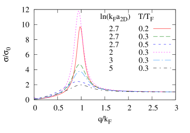
Figure 1: (Color online) Ratio of in-medium and free-space cross-section for total momentum $k$=0 as a function of the relative momentum $q$ for various combinations of interaction strength $\ln(k_{F}a_{2D})=\ln(2E_{F}/|E_{B}|)/2$ and temperature $T/T_{F}$.

we show the ratio of the in-medium cross section and the free-space one as a function of the relative momentum for a pair with $k=0$ for different values of interaction strength and temperature. At fixed interaction strength, there is a strong enhancement of the cross section when the temperature $T/T_{F}$ decreases, a precursor effect of superfluidity (cf. Fig. 2 of LABEL:Chiacchiera2009 for the 3D case, see also LABEL:AlmRoepke for the analogous effect in nuclear matter). This enhancement is most pronounced in the strongly interacting regime [small $\ln(k_{F}a_{2D})$]. Note that, throughout this paper, we consider only the fermionic regime in the normal phase, i.e., the case $\ln(k_{F}a_{2D})>0$ at temperatures above the superfluid transition temperature.

II.3 Method of phase-space moments

We look for approximate solutions of the Boltzmann equation using the method of phase-space moments. By fixing the functional form of $\Phi$ as

$$\Phi(\bm{\mathrm{r}},\bm{\mathrm{p}},t)=\sum_{j=1}^{n}c_{j}(t)\phi_{j}(\bm{\mathrm{r}},\bm{\mathrm{p}})\,,$$ (10)

the basis functions $\phi_{j}(\bm{\mathrm{r}},\bm{\mathrm{p}})$ being monomials in $\bm{\mathrm{r}}$ and $\bm{\mathrm{p}}$, one can obtain a closed set of $n$ coupled equations for the coefficients $c_{j}$ by multiplying Eq. (4) by $\phi_{i}$ and integrating over phase space. After Fourier transformation, the equations become algebraic and can be written in matrix form as $\sum_{j=1}^{n}A_{ij}(\omega)c_{j}(\omega)=a_{i}$, where $A$ is related to the transport and collision part and $a$ to the perturbation $\delta V$, see Refs. Chiacchiera2011 ; Pantel2012 . Once the coefficients $c_{i}$ are found, the deviation of any one-body observable from its equilibrium value, $\delta\langle q\rangle=\langle q\rangle-\langle q\rangle_{\mathit{eq}}$, can be expressed in the form $\delta\langle q\rangle=\sum_{i=1}^{n}b_{i}c_{i}$, $b_{i}$ being appropriate projections of the observable on the basis.

The choice of the $\phi_{i}$, of the excitation $\hat{V}$ and of the observable $\langle q\rangle$ depends on the mode one is interested in. In general, the response function $\langle q\rangle_{\mathit{pulse}}(\omega)=\delta\langle q\rangle(\omega)$ for the $\delta$-pulse excitation, Eq. (5), has $n$ poles at complex frequencies $\omega_{i}$. In simple cases, the real and imaginary parts of $\omega_{i}$ can directly be interpreted as the frequency and damping rate of the collective mode, as it was done, e.g., in LABEL:Baur2013. In general, however, it is necessary to analyse the full response function in order to extract the frequency $\omega$ and damping rate $\Gamma$ of the collective mode Chiacchiera2011 .

In the present paper, we will follow as closely as possible the experimental procedure. Note that in real experiments the mode is not excited by a $\delta$ pulse of the form Eq. (5), but the perturbation is adiabatically switched on and then suddenly switched off at $t=0$. The corresponding response $\langle q\rangle_{\mathit{step}}$ can easily be calculated (see appendix for more details) if the response $\langle q\rangle_{\mathit{pulse}}$ for the $\delta$ pulse is known. Then we fit the response $\langle q\rangle_{\mathit{step}}(t)$ with a function of the form

$$Q(t)=Ae^{-\Gamma t}\cos(\omega t+\varphi)+Be^{-\gamma t}\,,$$ (11)

as it is done in the analysis of the experimental data, in order to determine $\omega$ and $\Gamma$.

III Comparison between moments method and numerical calculations

In this section we will discuss the quadrupole mode in an isotropic harmonic trap, $V_{T}=\frac{1}{2}m\omega_{r}^{2}r^{2}$. The minimal ansatz function $\Phi$ is in this case given by

$$\Phi=c_{1}(x^{2}-y^{2})+c_{2}(p_{x}^{2}-p_{y}^{2})+c_{3}(xp_{x}-yp_{y})\,.$$ (12)

The excitation operator is $\hat{V}\propto x^{2}-y^{2}$ and the observable is the quadrupole moment of the cloud, $\langle q\rangle=\langle x^{2}-y^{2}\rangle$. This defines the method of moments at second order. Within this approximation, the frequency and damping rate of the quadrupole mode depend only on a single parameter, the average relaxation time $\tau$ Baur2013 . In the hydrodynamic limit $\tau\to 0$, one finds $\omega\to\sqrt{2}\omega_{r}$ and $\Gamma\to 0$. In the collisionless limit $\tau\to\infty$, one finds $\omega\to 2\omega_{r}$ and $\Gamma\to 0$. The maximum damping of $\Gamma\sim 0.354\omega_{r}$ is reached for $\tau\sim 0.471/\omega_{r}$. Hence, whether one includes a medium-modified cross section or not changes only the dependence of $\tau$ on $a_{2D}$, $T$ etc., but it cannot lead to a damping rate higher than $0.354\omega_{r}$, which is far below the observed maximum damping of $\sim 0.6\omega_{r}$ Vogt2012 .

In the 3D case, we have shown by comparing with numerical simulations that the second-order method overestimates the collision effects Lepers2010 . In the 2D case, the results of numerical calculations are already available WuZhang2012_2d . Although they still use a relaxation-time approximation, they include the essential effect that is missing in the second-order method, namely the position-dependence of the local relaxation time $\tau(\bm{\mathrm{r}})$. Since $\tau(\bm{\mathrm{r}})$ depends on collisions, it strongly increases if one goes from the trap center (high density) to the surface of the gas (low density).

As discussed in Refs. Lepers2010 and Chiacchiera2011 , this effect is automatically taken into account if one extends the method of moments to higher orders. As in the 3D case, we will include all the relevant moments up to fourth order , i.e.

$$\Phi=c_{1}(x^{2}-y^{2})+c_{2}(p_{x}^{2}-p_{y}^{2})+c_{3}(xp_{x}-yp_{y})\\ +c_{4}r^{2}(x^{2}-y^{2})+c_{5}r^{2}(p_{x}^{2}-p_{y}^{2})+c_{6}r^{2}(xp_{x}-yp_{y})\\ +c_{7}p^{2}(x^{2}-y^{2})+c_{8}p^{2}(p_{x}^{2}-p_{y}^{2})+c_{9}p^{2}(xp_{x}-yp_{y})\\ +c_{10}\bm{\mathrm{r}}\cdot\bm{\mathrm{p}}(x^{2}-y^{2})+c_{11}\bm{\mathrm{r}}\cdot\bm{\mathrm{p}}(p_{x}^{2}-p_{y}^{2})\,.$$ (13)

Let us now compare the second- and fourth-order results with the numerical results of LABEL:WuZhang2012_2d. The damping rate $\Gamma$ as function of the interaction strength $\ln(k_{F}a_{2D})$ is shown for different temperatures in Fig. 3.

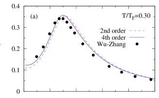
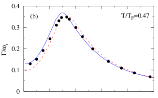
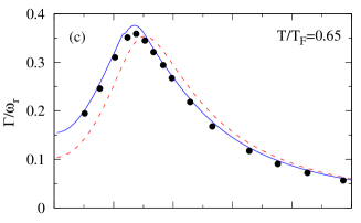
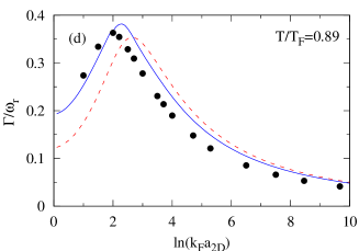
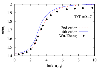
Figure 2: (Color online) Damping rate $\Gamma$ of the quadrupole mode as a function of the interaction strength for a system of $N=3500$ ⁴⁰K atoms with the free-space cross section in a harmonic isotropic trap with $\omega_{r}=2\pi\times 125$ Hz at different temperatures: (a) $T/T_{F}=0.3$, (b) 0.47, (c) 0.65, (d) 0.89. Dashed lines: second-order moments, solid lines: fourth order moments, points: numerical results by Wu and Zhang WuZhang2012_2d .

Figure 3: (Color online) Frequency $\omega$ of the quadrupole mode as a function of the interaction strength. The parameters of the system and the meaning of the different lines are the same as in Fig. 3(b).

For the sake of comparison, we used the free-space cross section in our calculation, and we also removed the constant shift of $0.05\omega_{r}$ from the numerical damping rates that was added in LABEL:WuZhang2012_2d to account in a simple way for the anharmonicity of the experimental trap potential (anharmonicity effects will be discussed in detail in the next section). We observe that within the second-order moments method (dashed lines) the transition from hydrodynamic to collisionless behavior, i.e., the maximum of $\Gamma$, lies at slightly weaker interaction [larger $\ln(k_{F}a_{2D})$] than within the numerical calculation (points). This is in line with our results for 3D, where the second-order method overestimates the collision effects, too Lepers2010 . The fourth-order results are in very good agreement with the numerical ones, especially at higher temperature [Figs. 3(c) and (d)], where the difference between the second- and fourth-order results becomes more pronounced.

In Fig. 3 we also show the frequency $\omega$ as function of $\ln(k_{F}a_{2D})$ for the temperature $0.47T_{F}$ for which numerical results are available. At first glance it looks as if the numerical result was in better agreement with the second-order calculation than with the fourth-order one. However, one sees that in the weakly interacting regime the numerical frequency stays systematically $2\%$ below both the second- and the fourth-order results. If we multiply the numerical frequencies by 1.02, they lie between the second- and fourth-order results in the range $\ln(k_{F}a_{2D})\geq 2$.

In conclusion, the second-order method overestimates the role of collisions. Especially at higher temperatures, the inclusion of fourth-order moments reduces the effects of collisions and significantly improves the agreement between the damping rates obtained within the method of moments and those obtained from a numerical calculation. However, at low temperatures, the corrections due to fourth-order moments are small.

IV Comparison with experiment

IV.1 Effect of the in-medium cross section

From now on, we will concentrate on results obtained with the fourth-order method, and compare them with the experiment of Refs. Vogt2012 ; Baur2013 . As a first step, we approximate the experimental system again by an isotropic harmonic trap with $\omega_{r}=2\pi\times 125$ Hz. In contrast to the preceding section, we will now include the in-medium cross section into the collision term. Within the moments method this is feasible, while it would be tremendously time-consuming in a numerical simulation like that of LABEL:WuZhang2012_2d.

In Fig. 4, we show the frequency and damping rate of the quadrupole mode as functions of the interaction strength for the case of $N=4300$ atoms ($E_{F}=h\times 8.2$ kHz) at $T/T_{F}=0.47$.

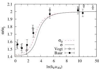
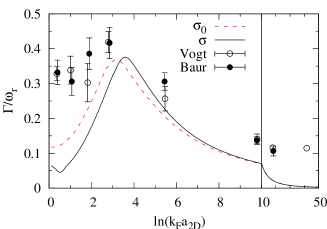
Figure 4: (Color online) Frequency (top) and damping rate (bottom) of the quadrupole mode in a harmonic isotropic trap containing $N=4300$ atoms at $T/T_{F}=0.47$. The dashed and solid lines represent fourth-order results obtained with the free-space and in-medium cross sections, respectively. The experimental data are taken from Refs. Vogt2012 and Baur2013 .

Since the in-medium cross section is enhanced, its main effect is that the system is more hydrodynamic (weaker damping) for strong interactions [small values of $\ln(k_{F}a_{2D})$] and the transition to the collisionless regime (maximum damping) takes place at weaker interactions [higher values of $\ln(k_{F}a_{2D})$] than with the free-space cross section. A similar effect of the in-medium cross section was already found in LABEL:Baur2013 within the second-order method (cf. Fig.  2 of LABEL:Baur2013). Concerning the agreement with the experimental data, one notes that the frequencies are qualitatively correctly described, but the rise from the hydrodynamic to the collisionless frequency happens at too weak interaction, and the disagreement gets worse if the in-medium cross section is used instead of the free-space one. The theoretical results for the damping are significantly too weak in almost the whole range of $\ln(k_{F}a_{2D})$, especially in the very weakly interacting regime [$\ln(k_{F}a_{2D})\gtrsim 10$].

IV.2 Realistic trap potential

As mentioned before, the damping of the quadrupole mode one obtains with the second-order method cannot exceed $0.354\omega_{r}$, independently of the cross section that is used in the collision term. In the fourth-order method, the damping can be somewhat stronger, but it stays far below the maximum damping $0.6\omega_{r}$ that was observed in one case in the experiment by Vogt et al. Vogt2012 . Furthermore, in this experiment, the quadrupole mode remains damped in the limit of vanishing interaction strength. This clearly shows that there are other sources of damping than the collision term, for instance the anharmonicity of the trap potential and the broken rotational symmetry. (By the way, damping of collective modes in the non-interacting gas was also observed in 3D, for instance in LABEL:Kinast2004 where it was consistent with the trap anharmonicity.)

In LABEL:Pantel2012, we showed that in 3D the damping of the sloshing mode in an anharmonic potential could be described within the method of moments once moments of higher order were included. Therefore we expect that the inclusion of higher-order moments in the description of the quadrupole mode will also allow us to describe its additional damping in an anharmonic trap.

The breaking of rotational invariance leads to a coupling of modes of different multipolarity, that can also result in an additional damping. For instance, in LABEL:Baur2013, the coupling of quadrupole and monopole (breathing) modes caused by the small ellipticity of the trap potential was studied. In an elliptic trap, the monopole mode and the two degenerate quadrupole modes (in 2D) are replaced by three new eigenmodes that have all different frequencies. Notice that a beat caused by the superposition of two eigenmodes with slightly different frequencies looks like a damping if the oscillation is only observed during a short time interval, as it is usually the case.

In the experiment Vogt2012 there is another effect that might play a role. Since the $z$ direction of the laser beam generating the potential is horizontal, the additional gravitational potential shifts the minimum of the potential downwards. While this would not have any effect in a purely harmonic potential, it leads in the anharmonic case to a potential that is no longer symmetric about its minimum. As a consequence, modes with opposite parity (e.g., sloshing and breathing) will be coupled. Actually, the symmetry in $x$ direction is broken, too, because of the presence of magnetic field gradients that shift the minimum in both $x$ and $y$ directions Vogt_Thesis .

We write our model potential as

$$\tilde{V}_{T}(\tilde{\bm{\mathrm{r}}})=-V_{0}e^{-2(\tilde{x}^{2}/w_{x}^{2}+\tilde{y}^{2}/w_{y}^{2})}-(m\bm{\mathrm{g}}+\mu\bm{\nabla}B)\cdot\tilde{\bm{\mathrm{r}}}\,,$$ (14)

where $V_{0}$ is the depth of the Gaussian potential, $w_{x}$ and $w_{y}$ are the waists of the laser beam in $x$ and $y$ directions, $\bm{\mathrm{g}}=-g\bm{\mathrm{e}}_{y}$ is the gravitational acceleration ($g=9.81$ m$/$s²), $\mu$ is the magnetic moment (approximately equal to the Bohr magneton $\mu_{B}$ in the case of alkali atoms), and $B=|\bm{\mathrm{B}}|$ is the strength of the magnetic field. For the sake of simplicity, we shift the minimum of the potential to the origin by defining $\bm{\mathrm{r}}=\tilde{\bm{\mathrm{r}}}-\bm{\mathrm{r}}_{0}$ and

$$V_{T}(\bm{\mathrm{r}})=\tilde{V}_{T}(\bm{\mathrm{r}}_{0}+\bm{\mathrm{r}})-\tilde{V}_{T}(\bm{\mathrm{r}}_{0})\,,$$ (15)

where $\bm{\mathrm{r}}_{0}=(x_{0},y_{0})$ is related to $\bm{\mathrm{g}}$ and $\bm{\nabla}B$ by

$$mg_{i}+\mu\nabla_{i}B=\frac{4V_{0}r_{0i}}{w_{i}^{2}}e^{-2(x_{0}^{2}/w_{x}^{2}+y_{0}^{2}/w_{y}^{2})}\quad(i=x,y)\,.$$ (16)

The average trap frequency $\bar{\omega}_{r}$ can be obtained from

$$m\bar{\omega}_{r}^{2}=\begin{vmatrix}\frac{\partial^{2}V_{T}}{\partial x^{2}}&\frac{\partial^{2}V_{T}}{\partial x\partial y}\\ \frac{\partial^{2}V_{T}}{\partial x\partial y}&\frac{\partial^{2}V_{T}}{\partial y^{2}}\end{vmatrix}_{\bm{\mathrm{r}}=0}^{1/2}\\ =\frac{4V_{0}}{w_{x}w_{y}}\sqrt{1-\frac{4x_{0}^{2}}{w_{x}^{2}}-\frac{4y_{0}^{2}}{w_{y}^{2}}}e^{-2(x_{0}^{2}/w_{x}^{2}+y_{0}^{2}/w_{y}^{2})}\,.$$ (17)

Using the parameters of the experiments Vogt2012 ; Vogt_Thesis , we obtain the potential shown in the upper panel of Fig. 5.

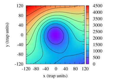
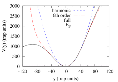
Figure 5: (Color online) Trap potential in units of $\hbar\bar{\omega}_{r}$ as function of $x$ and $y$ in units of $l_{\mathit{ho}}$ (top) and as function of $y$ for $x=0$ (bottom). We have used $\bar{\omega}_{r}=2\pi\times 125$ Hz Vogt2012 and $w_{x}=139$ $\mu$m, $w_{y}=142$ $\mu$m, $\nabla_{x}B=3.2$ G$/$cm and $\nabla_{y}B=-0.75$ G$/$cm Vogt_Thesis (as a consequence, $V_{0}=2617\hbar\omega_{r}$, $x_{0}=4.8l_{\mathit{ho}}$, and $y_{0}=-12.2l_{\mathit{ho}}$). Solid line: potential according to Eq. (14), dashed line: harmonic approximation, dash-dotted line: Taylor expansion up to sixth order. The Fermi energy $E_{F}$ corresponding to $N=4300$ atoms is shown as the dotted line.

As one can clearly see, the principal axes of the potential near the minimum are not aligned with the $x$ and $y$ axes. The trap frequencies along the principal axes are split by approximately 5%.

As explained in LABEL:Pantel2012, it is strictly speaking not possible to calculate the chemical potential $\mu_{0}$ as a function of the particle number $N$ if the potential does not go to $+\infty$ for $r\to\infty$. We avoid this problem in the same way as in LABEL:Pantel2012 by expanding the potential up to sixth order (i.e., keeping terms $\propto x^{k}y^{l}$ with $k+l\leq 6$) around $r=0$. In the present case, this expansion is very accurate up to energies of about ten times the Fermi energy. This is illustrated in the lower panel of Fig. 5.

As mentioned above, the asymmetry of the potential leads to a coupling between all kinds of modes, even those of different parity. If we want to describe this in the framework of the moments method, we have to make the most general ansatz, i.e., include all possible moments up to a given order. Our ansatz for $\Phi$ contains now 70 terms (1 of zeroth order, 4 of first order, 10 of second order, 20 of third order and 35 of fourth order) and reads

$$\Phi(\bm{\mathrm{r}},\bm{\mathrm{p}},t)=\sum_{k+l+m+n\leq 4}c_{klmn}(t)\phi_{klmn}(\bm{\mathrm{r}},\bm{\mathrm{p}})$$ (18)

where $k,l,m$ and $n$ are non-negative integers and

$$\phi_{klmn}(\bm{\mathrm{r}},\bm{\mathrm{p}})=x^{k}y^{l}p_{x}^{m}p_{y}^{n}\,.$$ (19)

The zeroth-order (constant) term is necessary for the conservation of the particle number during the oscillation Babadi2012 . This choice of $\Phi$, together with the same excitation operator and observable as before, $\hat{V}\propto x^{2}-y^{2}=q$, define our method at fourth order.

In Fig. 6

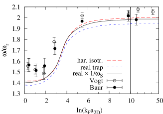
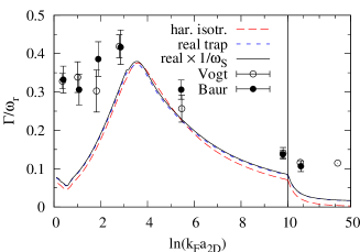
Figure 6: (Color online) Fourth-order results with in-medium cross section for the frequency (top) and damping rate (bottom) of the quadrupole mode in a trap containing $N=4300$ atoms at $T/T_{F}=0.47$. Long and short dashes represent, respectively, results for a harmonic isotropic trap and for the realistic trap shown in Fig. 5. The solid lines are the results for the realistic trap, normalized, as in the experiment, by the average sloshing frequency $\omega_{S}\approx 0.98\omega_{r}$ instead of $\omega_{r}$ given by Eq. (17). The experimental data are taken from LABEL:Vogt2012 (empty circles) and Baur2013 (filled circles).

we display results obtained within the full calculation (moments up to fourth order, in-medium cross section) for the case of a harmonic isotropic trap (long dashes) and for the realistic trap (short dashes and solid lines). One can see that the damping in the weakly interacting limit [$\ln(k_{F}a_{2D})\gtrsim 10$] is significantly enhanced in the realistic trap. Actually, the main reason for the additional damping $\Gamma$ is not the anharmonicity but the ellipticity of the trap. As discussed in the beginning of this subsection, this effect was already considered in Baur2013 but not analyzed in the same way. In our analysis, the beat caused by the two quadrupole modes that do no longer have the same frequencies results in a finite damping rate $\Gamma$ when the response is fitted with a single damped cosine function, Eq. (11), on a relatively short time interval. However, the effect is far too weak to explain the experimentally observed damping. At smaller values of $\ln(k_{F}a_{2D})$, the damping is not substantially modified by the anharmonicity and ellipticity of the trap.

The main effect of the anharmonicity is to reduce the frequency of the quadrupole mode (cf. the short and long dashed lines in the upper panel of Fig. 6). This looks incompatible with the data. However, if we normalize our quadrupole mode frequency, as in the experiment, by the average sloshing frequency $\omega_{S}=0.98\omega_{r}$ instead of the average trap frequency defined by the second derivatives at the minimum, Eq. (17), this effect disappears (solid line) because the anharmonicity reduces quadrupole and sloshing frequencies by approximately the same factor.

The damping rates of the quadrupole mode for other temperatures are shown in Fig. 7.

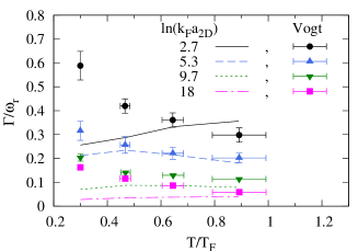
Figure 7: (Color online) Damping rates of the quadrupole mode in a realistic trap as functions of temperature for different interaction strengths. The lines represent fourth-order results with in-medium cross section in the realistic trap potential. The data points are taken from LABEL:Vogt2012. The particle numbers for $T=0.3,0.47,0.65$, and $0.89\,T_{F}$ are, respectively, $N=2620,4300,5180$, and $5300$, corresponding to the Fermi energies given in LABEL:Vogt2012.

To be consistent with the experiment, for each temperature the calculations are performed with a different value of $N$ (see caption of Fig. 7). The agreement between theory and data varies from each data point to the other, but two clear trends are visible: First, the experimentally observed damping is much stronger than the theoretical result at low temperature, $T/T_{F}=0.3$, for all values of the interaction strength. Second, the experimental damping in the weakly interacting case, $\ln(k_{F}a_{2D})\geq 9.7$, is also stronger than the theoretical one for all temperatures. Surprisingly, the experimental damping rate in the weakly interacting limit decreases with increasing temperature, while one would expect the opposite behavior if this damping was related to anharmonicity effects [cf. dashed-dotted line corresponding to $\ln(k_{F}a_{2D})=18$].

IV.3 Other possible effects

As we have seen, the agreement between theory and data is not satisfactory. While one maybe cannot trust the Boltzmann equation in the limit of strong interaction, it should at least be valid at large $\ln(k_{F}a_{2D})$, but even there a systematic disagreement between the theoretical and experimental damping rates persists. Possible effects one might think of are:

1. The excitation $\hat{V}$ is not of the form $x^{2}-y^{2}$, but it consists in squeezing the laser in one direction and stretching it in the other direction. This leads to anharmonic terms. In addition, it shifts the minimum of the potential and thereby excites not only the quadrupole but also the sloshing mode.

2. The observable $q$ is not $x^{2}-y^{2}$, but it is the quadrupole moment of the cloud after a free expansion during a time of flight (TOF) $t_{TOF}=12$ ms. This can easily be modeled, one just has to replace $x$ by $x+t_{\mathit{TOF}}p_{x}/m$ and analogously for $y$.

3. In the experiment, there is not a single 2D gas, but about 30 layers (“pancakes”) containing different particle numbers. The measured response is the sum of the responses of all of these layers. In LABEL:Vogt2012 it was suggested that the dephasing between the different layers might be an explanation of the observed damping.

The effects (a) and (b) do not change the eigenvalues, i.e., the poles $\omega_{i}$ of the response function in the complex plane, but they change the relative weight of the different eigenvalues and therefore have some effect if one determines the quadrupole frequency $\omega$ and damping rate $\Gamma$ by fitting the response function. In this respect, we note that, since with the full perturbation also a sloshing mode is excited, the fitting function has to be extended to take it into account. We studied in detail the case $T/T_{F}=0.47$ and found that in the collisionless regime [$\ln(k_{F}a_{2D})\gtrsim 7$] the results of the fits are not significantly changed. In the transition region from the hydrodynamic to the collisionless regime around $\ln(k_{F}a_{2D})=4$ the effect (a) tends to increase $\Gamma$ (by $\lesssim 10\%$) while (b) reduces it (by $\lesssim 10\%$), so that the net effect is even smaller. In the strongly interacting (near-hydrodynamic) regime [$\ln(k_{F}a_{2D})\lesssim 2$] the Fermi-surface deformation gets so weak that the corresponding quadrupole moment after the TOF is comparable with the quadrupole moment of the cloud before the TOF. Since both oscillate out of phase, the resulting amplitude can become very weak and the fit for the determination of $\omega$ and $\Gamma$ fails. In all three cases, the result of the fit depends very sensitively on details such as how the center-of-mass motion is taken into account.

We also studied (c) the possible dephasing of the different layers. When summing up the responses of layers having a distribution of particle numbers as shown in Fig. 3.7(a) of LABEL:Froehlich_Thesis, we found that the total response is strongly dominated by the central layers having the largest numbers of particles, since these have also the largest radii. As a consequence, the effect of the peripheral layers on the fitted frequency and damping rate is very weak. For example, we studied the case $\ln(k_{F}a_{2D})=3$, $T/T_{F}=0.28$. Since this case is right in between the hydrodynamic and the collisionless regimes, the frequency is supposed to depend strongly on the parameter $\ln(k_{F}a_{2D})$ that changes from one layer to the next because of the different particle number in each layer. One might therefore think that the dephasing could be important. Nevertheless we found that by summing the responses of all the layers [weighting each response with the particle number of the corresponding layer to compensate the factor $1/N$ in Eq. (1)] the frequency and damping rate changes only by $\sim 2\%$.

V Conclusions

We studied the quadrupole mode of a normal-fluid 2D trapped Fermi gas in the framework of the Boltzmann equation. The Boltzmann equation was solved approximatively within the method of phase-space moments. We showed that by including moments of up to fourth order in $\bm{\mathrm{r}}$ and $\bm{\mathrm{p}}$, we could nicely reproduce the results of the numerical study of LABEL:WuZhang2012_2d. In contrast to the 3D case Lepers2010 , the second-order moments alone were already in good agreement with the numerical results, and the effect of the fourth-order moments was quite small.

In order to compare with the experimental data of Refs. Vogt2012 and Baur2013 , we then included the in-medium cross section, calculated within the ladder approximation Enss2012 , into the collision integral. In LABEL:Enss2012, a rough estimate based on the shear viscosity of the uniform gas suggested that the inclusion of the in-medium cross section instead of the free-space one could result in a much stronger damping of the quadrupole mode. However, in agreement with Baur2013 , we found that the effect of the in-medium cross section was much less dramatic and consisted mainly in shifting the transition from the hydrodynamic to the collisionless regime to slightly weaker interactions or higher temperatures. The strong damping rates observed in the experiment for $\ln(k_{F}a_{2D})=2.7$ at $T/T_{F}=0.3$ and $0.47$ cannot be reproduced by our calculation.

There is also a strong discrepancy between theoretical and experimental damping rates in the (almost) collisionless regime. In an attempt to reconcile the theoretical results for the damping with the much stronger damping observed in the experiment in this regime, we included also the anharmonic shape of the experimental trap potential into our calculation. In LABEL:Pantel2012, we were able to explain in this way the experimentally observed damping of the sloshing mode in 3D. In the present 2D case, however, it turned out that the anharmonicity effects were very weak and did not substantially increase the damping of the quadrupole mode. Other effects, such as the expansion of the cloud or the summation over many 2D gases in the optical lattice, were not able to explain the experimental data either.

In the strongly interacting regime ($0\lesssim\ln(k_{F}a_{2D})\lesssim 1$), it is maybe not so surprising that the Boltzmann equation does not reproduce the experimental data, since one might still be at the edge of the pseudogap phase Feld2011 where the quasiparticle picture breaks down. However, it is very puzzling that it also fails to describe the data in the weakly interacting case. Actually, in the experiment Vogt2012 , a finite damping of the quadrupole mode persists even in the non-interacting limit [$\ln(k_{F}a_{2D})=545$]. Since all effects considered in the present paper were too weak to explain this damping, it must come from a different mechanism which has not yet been identified.

Appendix A Response function and determination of frequency and damping rate

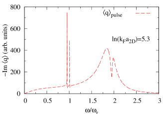
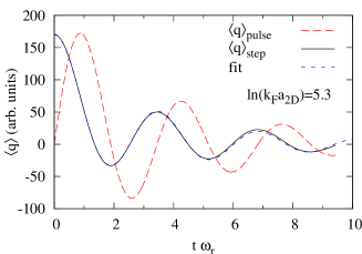
Figure 8: (Color online) Example for response functions in the frequency (top) and time (bottom) domains. The upper panel shows $-\operatorname{Im}\langle q\rangle_{\mathit{pulse}}(\omega)$ for the case $N=4300$, $T/T_{F}=0.47$, $\ln(k_{F}a_{2D})=5.3$ in the trap potential shown in Fig. 5. The lower panel shows the Fourier transform $\langle q\rangle_{\mathit{pulse}}(t)$ (long dashes), the corresponding $\langle q\rangle_{\mathit{step}}(t)$ (solid line) and the fit (short dashes) that yields the results $\omega=1.876\omega_{r}$ and $\Gamma=0.234\omega_{r}$.

As it was explained in Chiacchiera2011 and briefly mentioned in Sec. II.3, the moments method gives at higher order a number of complex eigenvalues $\omega_{i}$ whose real and imaginary parts cannot directly be interpreted as frequencies and damping rates of different collective modes. One rather has to look at the total response function. The response to the $\delta$-pulse perturbation Eq. (5) can be written in the form

$$\langle q\rangle_{\mathit{pulse}}(\omega)=\sum_{j=1}^{n}\frac{Z_{j}}{\omega-\omega_{j}}\,.$$ (20)

This is Eq. (25) of LABEL:Chiacchiera2011 if one replaces $\omega_{j}-i\Gamma_{j}$ by a complex frequency $\omega_{j}$. The complex frequencies $\omega_{j}$ satisfy $\operatorname{Im}\omega_{j}<0$ (in the case of a real $\omega_{j}$ one has to add an infinitesimal negative imaginary part). A Fourier transform gives

$$\langle q\rangle_{\mathit{pulse}}(t)=i\sum_{j=1}^{n}Z_{j}\,e^{-i\omega_{j}t}\,\theta(t).$$ (21)

The response to a more realistic excitation which is adiabatically switched on at $t=-\infty$ and which is suddenly switched off at $t=0$ is given by

$$\langle q\rangle_{\mathit{step}}(t)=\int_{-\infty}^{0}dt^{\prime}\langle q\rangle_{\mathit{pulse}}(t-t^{\prime})=\sum_{j=1}^{n}\frac{Z_{j}}{\omega_{j}}e^{-i\omega_{j}t\,\theta(t)}\,.$$ (22)

Figure 8 shows a typical example for a response function in the frequency and time domains. As a function of $\omega$ (upper panel), the response $-\operatorname{Im}\langle q\rangle_{\mathit{pulse}}(\omega)$ has a couple of spikes near $\omega=1$ coming from the (weak) coupling between quadrupole and sloshing modes due to the asymmetry of the trap potential. The broad peak corresponding to the quadrupole mode has a sharp minimum near $\omega=2$ due to the interference between the contributions of two complex eigenvalues. There is no obvious prescription how to extract a unique $\omega$ and $\Gamma$ from this response, so we transform the response to the time domain (lower panel) and follow the method used in the analysis of the experiment Vogt2012 , i.e., we fit Eq. (11) (short dashes) to $\langle q\rangle_{\mathit{step}}(t)$ (solid line) on the interval between $t=0$ and $t=12$ ms $\approx 10/\omega_{r}$ Vogt_Thesis .

References

- (1) K. Martiyanov, V. Makhalov, and A. Turlapov, Phys. Rev. Lett. 105, 030404 (2010).
- (2) E. Vogt, M. Feld, B. Fröhlich, D. Pertot, M. Koschorreck, and M. Köhl, Phys. Rev. Lett. 108, 070404 (2012).
- (3) L. P. Pitaevskii, and A. Rosch, Phys. Rev. A 55, 853 (R) (1997).
- (4) G. M. Bruun, Phys. Rev. A. 85, 013636 (2012).
- (5) T. Schäfer, Phys. Rev. A 85, 033623 (2012).
- (6) T. Enss, C. Küppersbusch, and L. Fritz, Phys. Rev. A 86, 013617 (2012).
- (7) L. Wu and Y. Zhang, Phys. Rev. A 85, 045601 (2012).
- (8) S. K. Baur, E. Vogt, M. Köhl, G. M. Bruun, Phys. Rev. A 87, 043612 (2013).
- (9) S. Riedl, E. R. Sánchez Guajardo, C. Kohstall, A. Altmeyer, M. J. Wright, J. H. Denschlag, and R. Grimm, G. M. Bruun and H. Smith, Phys. Rev. A 78, 053609 (2008).
- (10) S. Chiacchiera, T. Lepers, D. Davesne, and M. Urban, Phys. Rev. A 79, 033613 (2009).
- (11) T. Lepers, D. Davesne, S. Chiacchiera, and M. Urban, Phys. Rev. A 82, 023609 (2010).
- (12) S. Chiacchiera, T. Lepers, D. Davesne, and M. Urban, Phys. Rev. A 84, 043634 (2011).
- (13) P.-A. Pantel, D. Davesne, S. Chiacchiera, and M. Urban, Phys. Rev. A 86, 023635 (2012).
- (14) M. Babadi and E. Demler, Phys. Rev. A 86, 063638 (2012).
- (15) E.M. Lifshitz and L.P. Pitaevskii, Physical Kinetics, Landau-Lifshitz Course of Theoretical Physics, vol. 10 (Pergamon, Oxford, 1980).
- (16) S. K. Adhikari, Am. J. Phys. 54, 362 (1986).
- (17) D. S. Petrov and G.V. Shlyapnikov, Phys. Rev. A 64, 012706 (2001).
- (18) T. Alm, G. Röpke, and M. Schmidt, Phys. Rev. C 50, 31 (1994); T. Alm, G. Röpke, W. Bauer, F. Daffin, and M. Schmidt, Nucl. Phys. A 587, 815 (1995).
- (19) J. Kinast, S. L. Hemmer, M. E. Gehm, A. Turlapov, and J. E. Thomas, Phys. Rev. Lett. 92, 150402 (2004).
- (20) E. Vogt, PhD Thesis, University of Cambridge (2013).
- (21) B. Fröhlich, PhD Thesis, University of Cambridge (2011).
- (22) M. Feld, B. Fröhlich, E. Vogt, M. Koschorreck, and M. Köhl, Nature 480, 75 (2011).